 Open Access Article
 This Open Access Article is licensed under a
 Creative Commons Attribution 3.0 Unported Licence
The limit of macroscopic homogeneous ice nucleation at the nanoscale†
John A.
Hayton
 a,
Michael B.
Davies
ab,
Thomas F.
Whale
cd,
Angelos
Michaelides
a and
Stephen J.
Cox
*a
a,
Michael B.
Davies
ab,
Thomas F.
Whale
cd,
Angelos
Michaelides
a and
Stephen J.
Cox
*a
aYusuf Hamied Department of Chemistry, University of Cambridge, Lensfield Road, Cambridge CB2 1EW, UK. E-mail: sjc236@cam.ac.uk
bDepartment of Physics and Astronomy, University College London, London WC1E 6BT, UK
cDepartment of Chemistry, University of Warwick, Gibbet Hill Road, Coventry CV4 7AL, UK
dSchool of Earth and Environment, University of Leeds, Leeds, UK
First published on 22nd June 2023
Abstract
Nucleation in small volumes of water has garnered renewed interest due to the relevance of pore condensation and freezing under conditions of low partial pressures of water, such as in the upper troposphere. Molecular simulations can in principle provide insight on this process at the molecular scale that is challenging to achieve experimentally. However, there are discrepancies in the literature as to whether the rate in confined systems is enhanced or suppressed relative to bulk water at the same temperature and pressure. In this study, we investigate the extent to which the size of the critical nucleus and the rate at which it grows in thin films of water are affected by the thickness of the film. Our results suggest that nucleation remains bulk-like in films that are barely large enough accommodate a critical nucleus. This conclusion seems robust to the presence of physical confining boundaries. We also discuss the difficulties in unambiguously determining homogeneous nucleation rates in nanoscale systems, owing to the challenges in defining the volume. Our results suggest any impact on a film’s thickness on the rate is largely inconsequential for present day experiments.
1 Introduction
The formation of ice from liquid water is one of the most important phase transitions on Earth, and plays a vital role in climate science,1–7 cryopreservation,8–10 geology11,12 and many industrial applications.13–16 For example, many properties of clouds are affected by the relative compositions of ice and water,3,17–19 and consequently, the accuracy of climate models rely heavily on parameterizations to predict ice nucleation in the atmosphere.Broadly speaking, when ice forms, it can do so either heterogeneously, where the surface of, say, a solid particle facilitates nucleation, or homogeneously, in the absence of such surfaces. Despite heterogeneous nucleation being by far more common, homogeneous nucleation is important when temperatures approach approx. −40 °C, e.g., in cirrus cloud formation in the upper troposphere.2,3,20–24 Yet, even in the absence of surfaces presented by solid particles, the finite volume occupied by the liquid means an interface (e.g., with vapor or oil) nonetheless remains. A long-standing issue for homogeneous nucleation has therefore been to establish whether nucleation is enhanced close to the liquid–vapor interface, or suppressed. Owing to the small length and fast times scales involved, however, it is experimentally challenging to establish whether homogeneous nucleation occurs near the interface, or in the bulk of the fluid. Molecular simulations have therefore been employed by several groups to investigate where in the liquid, homogeneous nucleation occurs.25–30 While pioneering simulation studies from Vrbka and Jungwirth25,26 suggested that nucleation is enhanced at the liquid–vapor interface, their results are likely affected by the finite size of the simulation cell.31 The broad consensus from multiple simulation studies is that ice formation occurs away from the interface, in regions of the fluid that are bulk-like. These conclusions are also supported by thermodynamic arguments made by Qiu and Molinero.32
If ice forms preferentially in the bulk of the liquid, what does this mean for the observed rate of ice nucleation? In 2013, using forward flux sampling, Li et al.27 found, upon decreasing the droplet radius from approx. 4.9 nm to approx. 2.4 nm, that nucleation rates at 230 K were decreased relative to that of bulk water by eight orders of magnitude; for radii ≳5 nm, nucleation rates were virtually indistinguishable from that of the bulk. With the exception of the smallest droplet investigated, this significant decrease of the rate upon decreasing the radius appeared to be explained well by the associated change in Laplace pressure. These findings were consistent with a previous study by Johnston and Molinero.28 However, subsequent simulation studies that investigated ice nucleation in thin water films,29,33 whose planar interfaces correspond to zero Laplace pressure, found that nucleation rates were noticeably suppressed relative to that of bulk, even for film thicknesses ≳5 nm. Owing to the computationally demanding nature of simulating ice formation, these studies used a coarse-grained representation of water’s interactions, the mW model.34 In this model, instead of explicitly representing the hydrogen bond network, the local tetrahedrality is enforced by a three body contribution to the potential energy function. Despite its simplicity, the mW model reasonably describes the anomalies and structure of water and its phase behavior, including the density maximum, the increase in heat capacity and compressibility of the supercooled region and melting temperatures of both hexagonal and cubic ice.34–37
To add further complication to the above apparent discrepancy between droplets and films, tour-de-force simulations employing the TIP4P/ice model,38 which unlike the coarse grained mW model, accounts explicitly for electrostatic interactions and water’s hydrogen bond network, found that nucleation in thin water films was increased relative to that of bulk water by approximately seven orders of magnitude.30 This increase was attributed to an increase in average crystalline order and cage-like structure for TIP4P/ice (in the liquid state) in a thin-film geometry, which even persisted in film thicknesses as large as 9 nm. These pronounced structural changes were not observed with the coarse grained mW model. While the origin of such a discrepancy might be attributed to a lack of essential physics in the coarse grained model, this may raise a question mark over the use of mW to investigate ice formation in confined geometries, despite its success,37,39,40e.g., in explaining ice nucleation from vapor via a pore condensation and freezing mechanism.41
In this article, we first aim to resolve this apparent discrepancy between the coarse grained mW model and the all-atom TIP4P/ice model. Then, in Section 3, using the computationally more efficient mW model, we directly assess how the simplest confining geometry of all—a thin film of water in contact with its vapor—impacts ice formation. In Section 4 we extend our investigation to a more realistic case where water is confined between two solid surfaces. We conclude our findings in Section 5. A broad overview of the methodology is described throughout the manuscript, with full details provided in Section 6 and the ESI.†
2 Structural properties of thin water films converge to their bulk values on a microscopic length scale
As discussed above, previous work from Haji-Akbari and Debenedetti,30 using the TIP4P/ice water model at 230 K reported that the nucleation rate J(W) in a film of thickness W ≈ 4 nm is roughly seven orders of magnitude larger than in bulk water, whose rate we denote as J(∞). This significant enhancement of the rate has been attributed to a structure of liquid water “deep” in the interior of thin films that is distinctly different from that found for homogeneous bulk water. In particular, measures of local order, as prescribed, e.g., by a Steinhardt order parameter42 for the ith water molecule, | (1) |
 | (2) |
![[r with combining circumflex]](https://www.rsc.org/images/entities/b_char_0072_0302.gif) ij is the unit vector pointing from molecule i to molecule j, and Y6m is the mth component of a sixth-rank spherical harmonic. Similarly, the number of cage-like structures was also found to be increased in thin water films. In contrast, when using the mW potential, such measures of local structure converge to their bulk values within approx. 1 nm of the interface.
ij is the unit vector pointing from molecule i to molecule j, and Y6m is the mth component of a sixth-rank spherical harmonic. Similarly, the number of cage-like structures was also found to be increased in thin water films. In contrast, when using the mW potential, such measures of local structure converge to their bulk values within approx. 1 nm of the interface.
In a recent study, Atherton et al.46 discussed the sensitivity of the melting point of simple point charge models such as TIP4P/ice, on the choice of cutoff, r*, for the non-electrostatic interactions between water molecules. There it was shown that decreasing r* led to a systematic increase in the melting temperature. More importantly, it was noticed that choices of r* typically used in molecular simulations effectively correspond to negative pressures of a few hundred bar, when compared to homogeneous bulk systems that use a mean-field treatment to correct for truncated interactions. This observation was argued to be particularly relevant when comparing nucleation in thin water films (where standard mean-field treatments of truncated interactions have no impact) to homogeneous bulk systems. In ref. 46, rough arguments based on results from Bianco et al.47 were used to suggest that this effective negative pressure was the root of faster ice nucleation in thin films, but firm evidence was lacking.
For a thin film of water in coexistence with its vapor, it can readily be argued that the pressure far from the interfaces is approximately 0 bar.48 Therefore, to obtain a suitable reference for the local structure in the homogeneous bulk fluid, we have performed simulations in the isothermal–isobaric ensemble at a temperature T = 230 K, and pressure p = 0 bar (see ESI† for full simulation details), and computed
 | (3) |
![[small rho, Greek, macron]](https://www.rsc.org/images/entities/i_char_e0d1.gif) is the density of bulk water, N is the number of water molecules in the simulation, and angled brackets indicate an ensemble average. An important detail is that, when using the TIP4P/ice potential, we have truncated and shifted non-electrostatic interactions at r* = 8.5 Å; following ref. 46 we indicate this molecular model as TIP4P/ice(8.5). We find 〈
is the density of bulk water, N is the number of water molecules in the simulation, and angled brackets indicate an ensemble average. An important detail is that, when using the TIP4P/ice potential, we have truncated and shifted non-electrostatic interactions at r* = 8.5 Å; following ref. 46 we indicate this molecular model as TIP4P/ice(8.5). We find 〈![[q with combining macron]](https://www.rsc.org/images/entities/i_char_0071_0304.gif) 6〉/ ≈ 0.266.
6〉/ ≈ 0.266.
We now turn our attention to a thin film, as shown in Fig. 1a, also at T = 230 K. The specific system we consider comprises 3072 TIP4P/ice(8.5) water molecules, and the lateral dimensions of the simulation cell are chosen such that W ≈ 4.3 nm. Throughout this paper, the width of a film is defined as W = N/A, where A is the cross-sectional area. W is then varied by changing A. This simple measure is roughly consistent with the separation of Gibbs dividing surfaces.
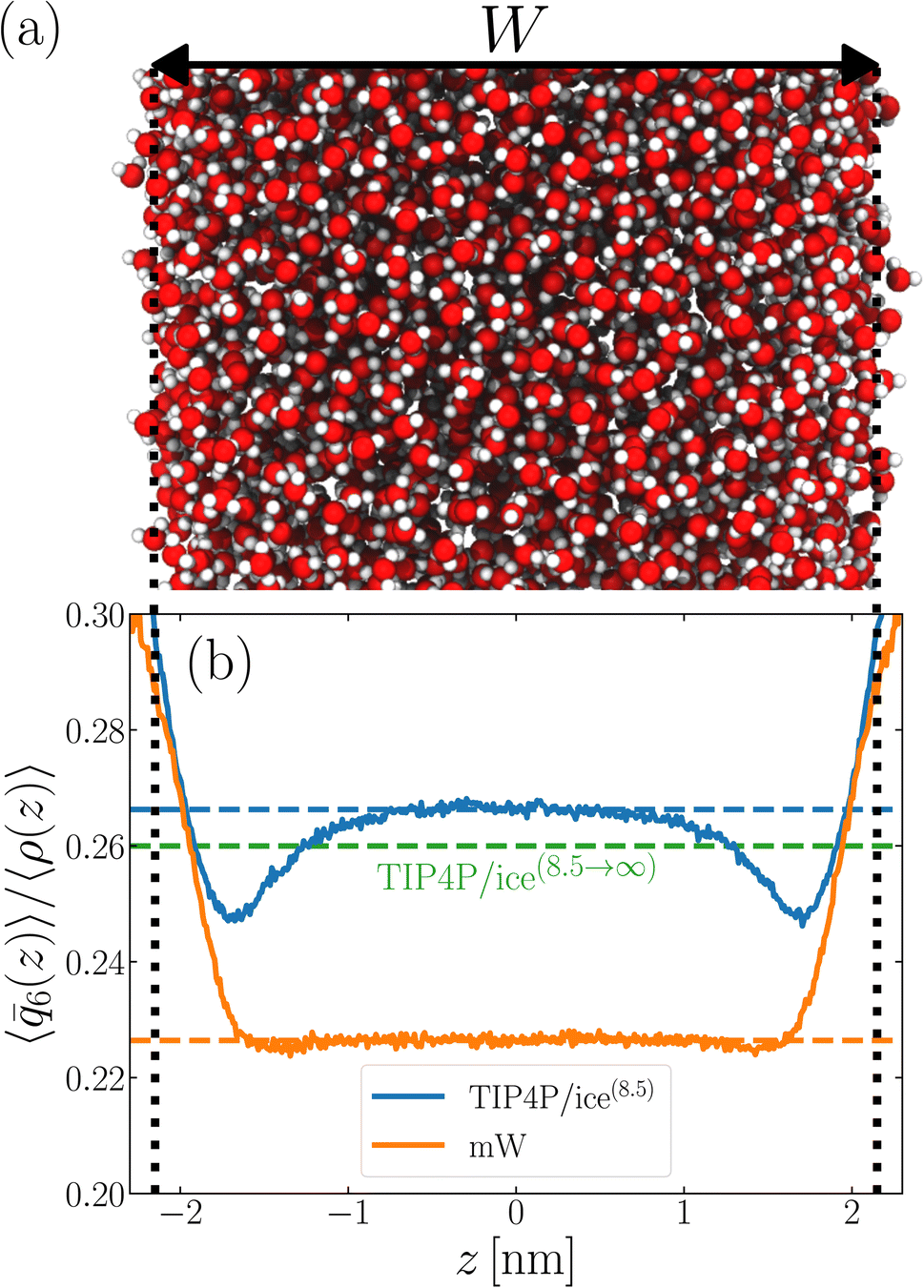 | ||
| Fig. 1 Structural properties of TIP4P/ice(8.5) and mW converge to their bulk values within approx. 1–1.5 nm of the liquid–vapor interface. (a) Snapshot of a TIP4P/ice(8.5) film of thickness W ≈ 4.3 nm at T = 230 K. The z axis (normal to the liquid–vapor interface) lies along the horizontal. Local structure away from the interface soon becomes bulk-like, as shown by 〈6(z)〉/〈ρ(z)〉 in (b) for TIP4P/ice(8.5) (blue) and mW (orange). Dashed lines show 〈6〉/ obtained from simulations of the bulk fluid at T = 230 K and p = 0 bar. When truncated interactions are accounted for in a mean-field fashion, a discrepancy in local structure in the center of the film and homogeneous bulk water emerges, as indicated by the dashed green line. The vertical dotted lines indicate the location of the liquid–vapor interface at z = ±W/2. | ||
To analyze the spatial variation in the structure of this film, we compute
 | (4) |
 | (5) |
6(z)〉/〈ρ(z)〉 ≈ 0.266 converges to its bulk value within approx. 1–1.5 nm of the interface, as indicated by the dashed blue line in Fig. 1b. In addition, the dashed green line shows 〈6〉/〈ρ(z)〉 ≈ 0.260 obtained from a simulation of the bulk fluid at T = 230 K and p = 0 bar, in which a mean-field treatment for truncated interactions has been employed; we denote this molecular model TIP4P/ice(8.5→∞). We see that the result obtained with TIP4P/ice(8.5→∞) lies, on average, below 〈6(z)〉/〈ρ(z)〉 obtained with TIP4P/ice(8.5).
Also shown in Fig. 1b is a similar analysis for the mW model. While we see quantitative differences with the TIP4P/ice(8.5) result, the important point is that 〈6〉/〈ρ(z)〉 ≈ 0.226 converges to its bulk value in the center of the film, on a similar length scale to TIP4P/ice(8.5). This result demonstrates that the structural differences between mW and TIP4P/ice that lead to apparently qualitative differences in nucleation rates can be resolved through a consistent treatment of truncated interactions. Combined with previous observations that the mechanism of ice formation in thin films is similar between the two models,27,29,30 the results in this section strongly suggest that the coarse-grained mW model likely contains the essential physics to describe ice nucleation in these systems.
In the following section, we will exploit the computational efficiency of the mW model to explore how the nucleation rate in thin water films depends upon W. Specifically, using the seeding technique, we will investigate how both the size of the critical nucleus and its growth depend upon W. Preliminary results for TIP4P/ice(8.5) with W = 4.3 nm are given in the ESI.†
3 Nucleation in thin water films remains bulk-like down to very small length scales
Having established consistency between TIP4P/ice(8.5) and mW in describing the structure of thin water films, we will now investigate the extent to which W impacts ice nucleation. To do so, we will make use of the ‘seeding’ method, first introduced by Bai and Li49,50 in their study of Lennard-Jones particles, and popularized for ice nucleation by Vega and co-workers.47,51–57 As the seeding approach has been detailed previously by others,51,52,54,55 here we will only briefly sketch an outline of the procedure.3.1 Investigating ice nucleation in thin water films with seeding simulations
The principal idea behind the seeding method is to initialize the system with a preformed ice nucleus (a ‘seed’) and observe whether the seed, on average, grows such that the system ends up as ice, or shrinks such that the system ends up as liquid water. If the seed is smaller than the critical ice nucleus, it will tend to melt, whereas if it is larger, it will tend to grow; the size of the critical ice nucleus can be determined from seeds that have equal tendency to grow or melt. In our case, this was achieved by first equilibrating a bulk crystal of hexagonal ice comprising 16![[thin space (1/6-em)]](https://www.rsc.org/images/entities/char_2009.gif) 000 molecules at 220 K and 0 bar, and then carving out a spherical cluster. The cluster was then inserted into the center of a thin film of liquid water of thickness W, which itself had been equilibrated at 220 K; this was done after first removing water molecules to create a spherical cavity of an appropriate size to accommodate the ice cluster. With the molecules in the ice cluster held fixed, the surrounding fluid was then relaxed by performing a short 80 ps molecular dynamics simulation. We subsequently calculated the size of the largest cluster of ice-like molecules in the system, ncl, which we took to define the size of our initial ice seed. An example of such a seed is shown in Fig. 2.
000 molecules at 220 K and 0 bar, and then carving out a spherical cluster. The cluster was then inserted into the center of a thin film of liquid water of thickness W, which itself had been equilibrated at 220 K; this was done after first removing water molecules to create a spherical cavity of an appropriate size to accommodate the ice cluster. With the molecules in the ice cluster held fixed, the surrounding fluid was then relaxed by performing a short 80 ps molecular dynamics simulation. We subsequently calculated the size of the largest cluster of ice-like molecules in the system, ncl, which we took to define the size of our initial ice seed. An example of such a seed is shown in Fig. 2.
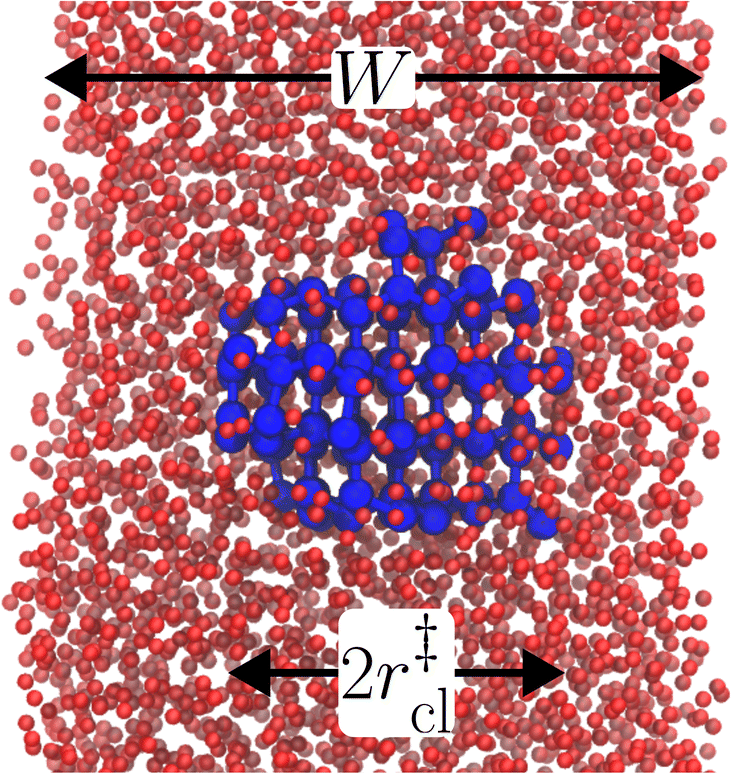 | ||
| Fig. 2 A snapshot from a seeding simulation with W = 3.5 nm after initial equilibration at T = 220 K, using the mW model. Molecules identified as belonging to the largest ice-like cluster are shown by large blue spheres, while all other molecules are shown by small red spheres. In this case, the initial seed happens to be critical, with approximate radius r‡cl, as indicated. | ||
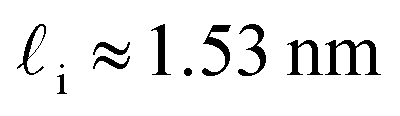
We have investigated film thicknesses in the range 2.5 nm ≲ W ≲ 6 nm, with N ≈ 6000 throughout (different thicknesses are achieved by varying A). For each W, approximately 700–900 seeding simulations were performed. The range of initial cluster sizes depended on film width, with 60 ≲ ncl ≲ 220 overall; this was sufficient to span both pre- and post-critical cluster sizes. In Fig. 3a, we present the probability pice(ncl; W) that a seed of size ncl goes on to form ice. The critical cluster size n‡cl is estimated from pice(n‡cl; W) = 0.5. We observe that for W ≳ 3.5 nm, n‡cl ≈ 120, which compares well to the value obtained in a bulk simulation of mW. To help give this result some perspective, the radius of these critical clusters is r‡cl ≈ 0.96 nm. If we consider W = 3.5 nm, this gives (W − 2r‡cl)/2 ≈ 0.8 nm, which is broadly in line with accepted thicknesses of the liquid–vapor interface.27,29,58 In other words, as soon as the films are thick enough to accommodate a bulk-like region, critical nuclei appear ambivalent to the nearby presence of the liquid–vapor interface. For W ≲ 3 nm, deviations of n‡cl from its bulk value are observed, with n‡cl ≈ 170 in the thinnest film investigated (W ≈ 2.5 nm). For all systems investigated, n‡clvs. W is plotted in Fig. 3b.
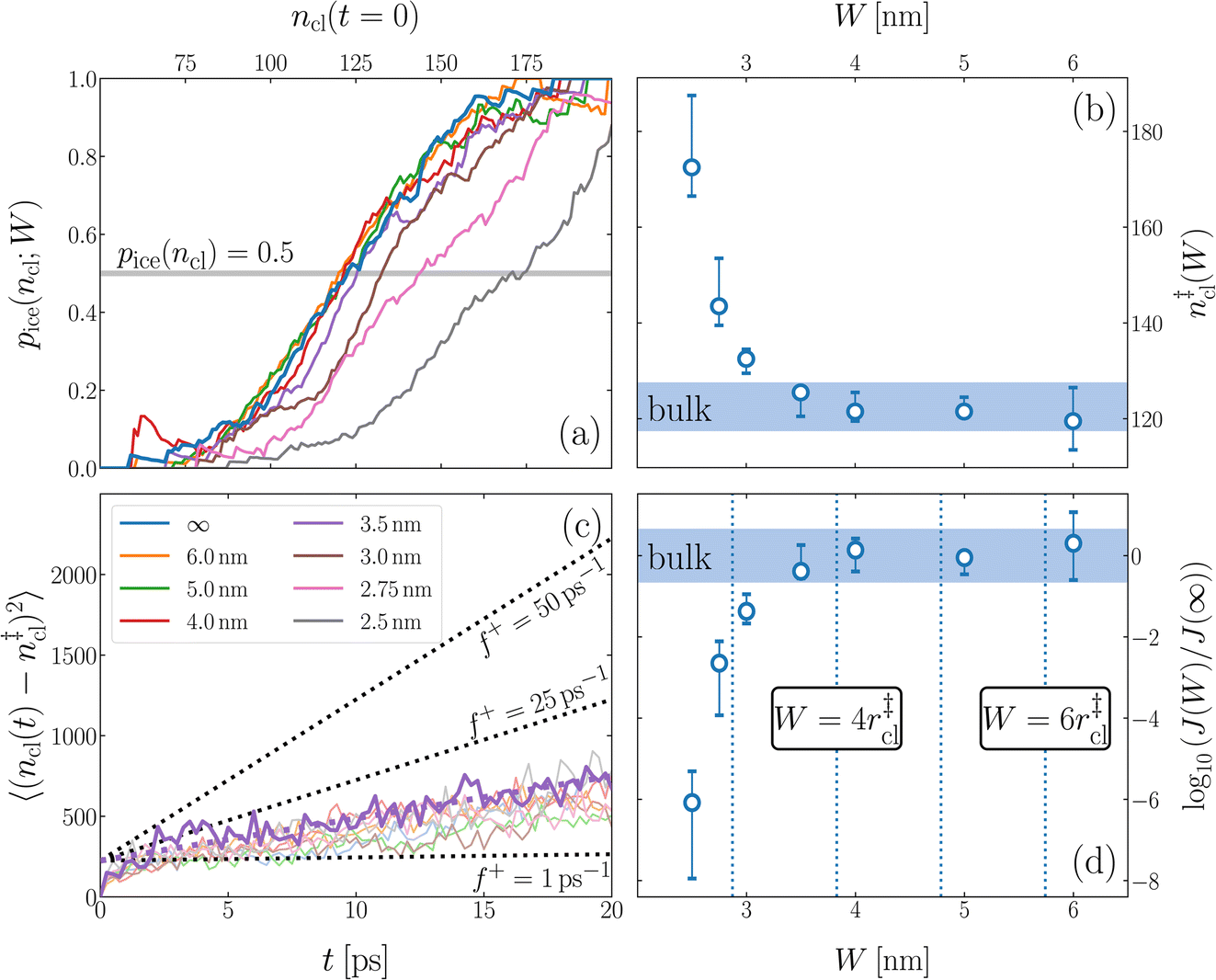 | ||
| Fig. 3 Assessing the impact of film width, W, on ice nucleation. (a) The size of the critical cluster for a given W [as indicated in the legend in (c)] is obtained by finding the size of cluster after initial equilibration, ncl(t = 0) = n‡cl, for which there is equal probability to grow or shrink, pice(ncl; W) = 0.5. We find that n‡cl only differs significantly from its value in bulk water for W ≲ 3.5 nm, as shown in (b). Error bars indicate the range of results obtained by splitting each data set into three. In (c) we show 〈(ncl(t) − n‡cl)2〉 for each W. The attachment frequency f+ is obtained by fitting a straight line after an initial transient period, as shown in bold for W = 3.5 nm. Dotted lines indicate hypothetical values of f+ to give a sense of scale. Using the obtained n‡cl and f+, and Δμ/kB = 122 K, the nucleation rate is obtained from eqn (6), as shown in (d). In panels (b) and (d), the shaded region indicates the result obtained from simulations of bulk water. | ||
Computation of nucleation rates with the seeding approach relies upon classical nucleation theory (CNT):49–52
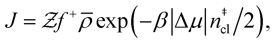 | (6) |
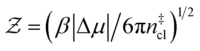 is the Zeldovich factor, and f+ is the attachment frequency. For the chemical potential difference, a range of values spanning approximately 118 K ≲ |Δμ|/kB ≲ 126 K have been reported in the literature59,60 and for simplicity, we take |Δμ|/kB = 122 K. (We have repeated the following analyses with the extremal values of this range, and find that the results are virtually indistinguishable [see ESI†].) As we have found that n‡cl remains roughly constant for W ≳ 3.5 nm, the remaining source for deviations of the rate from that of the bulk may lie in the dynamics, as codified by f+. In Fig. 3c we present the attachment frequency obtained from
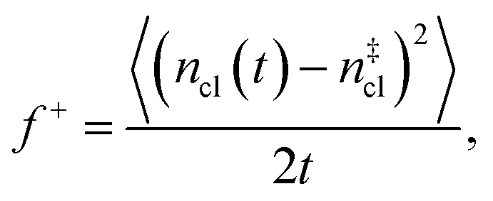 | (7) |
= 33.3774 nm−3), and is also reported in parentheses
| W [nm] | n ‡cl | f + [ps−1] | log10(J/(m−3 s−1)) |
|---|---|---|---|
| ∞ | 122.5(117.5–127.5) | 13.7 | 25.1(24.4–25.7) |
| 6.0 | 119.5(113.5–126.5) | 11.9 | 25.4(24.5–26.2) |
| 5.0 | 121.5(121.5–124.5) | 9.3 | 25.1(24.6–25.1) |
| 4.0 | 121.5(119.5–125.5) | 14.2 | 25.2(24.7–25.5) |
| 3.5 | 125.5(120.5–126.5) | 13.1 | 24.7(24.5–25.4) |
| 3.0 | 132.5(129.5–134.5) | 9.7 | 23.7(23.4–24.1) |
| 2.75 | 143.5(139.5–153.5) | 9.5 | 22.4(21.1–22.9) |
| 2.5 | 172.5(166.5–187.5) | 14.2 | 19.0(17.1–19.8) |
3.2 Comparing, and reconciling, results from seeding with previous studies
Despite good agreement of J(∞) with previous literature values, our results for W ∼ 5 nm are at odds with previous work. For example, using forward flux sampling, for mW under the same conditions, Haji-Akbari et al.29 found J(5 nm)/J(∞) ≈ 0.006. Similarly, by computing mean first passage times at 205 K, Lü et al.33 found that ice nucleation rates in thin water films were suppressed compared to that of the bulk. How can we rationalize this apparent discrepancy of our seeding simulations, which find that J(W)/J(∞) ≈ 1 once the film is thick enough to accommodate a critical nucleus? We, in fact, argue that this discrepancy is largely superficial. In the case of Lü et al., the reported impact of W on the rate was relatively modest, with J(5 nm)/J(∞) ≈ 0.5, within the range of uncertainty of our result. But there is also a more subtle aspect at play. Methods such as forward flux sampling and calculating the mean first passage time obtain a rate first by computing the probability to undergo a nucleation event per unit time in a particular sample, and then normalize by the volume of the sample. For homogeneous systems, the definition of this volume is unambiguous. In contrast, for inhomogeneous systems such as thin water films, what to take for the volume is less clear-cut, and J(W) becomes increasingly sensitive to this normalization procedure as W decreases. The seeding method, on the other hand, provides an estimate of the rate directly (see eqn (6)), albeit conditioned, in our study, on the nucleus forming in the bulk-like region. The advantage of the seeding method is that it clearly demonstrates that n‡cl and f+ remain roughly constant for W ≥ 3.5 nm. We note that in the ESI of Li et al.,27 who used forward flux sampling, the nucleation rate in a film comprising 4096 mW water molecules was found to be indistinguishable from that of the bulk; it appears that Li et al. account for the surface region in their normalization procedure.To help further understand the differences between J(W) computed with seeding and previous work, it is instructive to introduce the following simple model, which is similar to existing models introduced by others.27,33,65 We suppose that the thin film can be separated into two interfacial regions of thickness  that sandwich a central bulk-like region of thickness
  . Accounting for the volume occupied by the critical nucleus, the volume accessible for nucleation in the bulk-like region is
 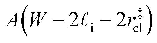 (see Fig. 4). In the remaining volume,
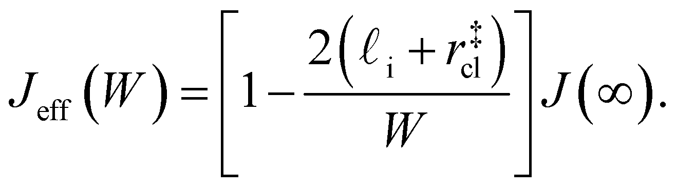
 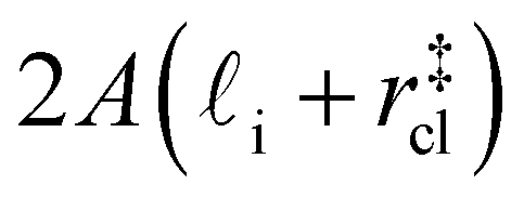 , we assume that nucleation occurs with a rate Ji. For a sample of total volume AW, the number of nuclei that form per unit time is determined by an effective nucleation rate Jeff:
 | (8) |
 | (9) |
 . While this order of magnitude is reasonable for an interfacial thickness, it is inconsistent with our finding that the size of critical nucleus remains constant for W ≳ 3.5 nm. As we did above, we can instead estimate
 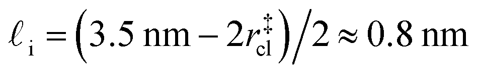 . For W = 5 nm, we then obtain Jeff(5 nm)/J(∞) ≈ 0.3. This more modest suppression in the rate appears comparable to that obtained at 205 K by Lü et al.33
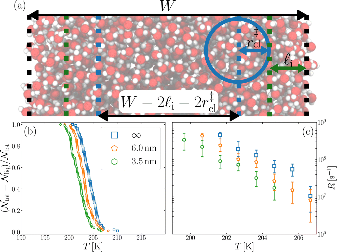 | ||
Fig. 4 Reconciling nucleation rates obtained from seeding with other approaches. (a) Schematic of the simple model described in the text. Nucleation is assumed to proceed in a bulk-like fashion in the central volume 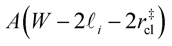 . In (b) we present the fraction of frozen samples for W/nm = 3.5 and 6, and bulk water. Each system comprises 6000 mW molecules and is cooled at a rate of 0.2 K ns−1 from an initial temperature of 220 K. There is a modest shift to lower temperatures with the films compared to bulk water. The freezing rate, R, for W = 3.5 nm, as shown in (c), differs at most by a factor of five compared to the bulk result. . In (b) we present the fraction of frozen samples for W/nm = 3.5 and 6, and bulk water. Each system comprises 6000 mW molecules and is cooled at a rate of 0.2 K ns−1 from an initial temperature of 220 K. There is a modest shift to lower temperatures with the films compared to bulk water. The freezing rate, R, for W = 3.5 nm, as shown in (c), differs at most by a factor of five compared to the bulk result. | ||
3.3 Probing the effective rate in thin water films through the lens of an experimentalist
What the above analysis demonstrates is the sensitivity of the effective nucleation rate to the interfacial thickness and the size of the critical nucleus r‡cl. While the latter is in principle a physical observable, there is a degree of arbitrariness in defining an interfacial thickness, which obfuscates direct interpretation of Jeff. In an attempt to gauge the significance of any suppression of Jeff with W, it is useful to think of an instance when one might be interested in ice formation in such small volumes, such as to understand how a porous material (or a rough surface with, e.g., cracks) might promote ice formation via a pore condensation and freezing mechanism.41,66–69 In such cases, one is probably less interested in the precise value of an effective rate, and instead more concerned whether ice can form, given that a pore/crack is filled with water under these conditions.
In this spirit, in Fig. 4b we present the fraction of frozen samples against temperature for bulk water, W = 6 nm and W = 3.5 nm, obtained by cooling 100 replicas of each system at 0.2 K ns−1. Note that the number of water molecules is the same in each case (6000 mW). The size of the largest ice-like cluster was monitored, and the system was considered frozen when the largest cluster ncl(T) ≥ 200.§ We see that the curves are shifted relative to each other, with the bulk samples freezing at the highest temperature, and the W = 3.5 nm film at the lowest temperature being separated by around 2 K. We are able to achieve statistically different freezing temperatures and rates in our studies primarily due the artificially high control we can exert on the number of molecules (N = 6000) and with it the volume undergoing cooling.
In experimental systems such fine control is impossible, and with it the deviations in freezing temperatures and freezing rates reported here become unimportant. To see this, we compare the impact of varying W by computing the freezing rate, R, for each of the data sets using an approach typically employed in the analysis of laboratory experiments.70R is analogous to the radioactive decay constant (a first-order reaction rate constant) and is most easily determined from experiments conducted on completely identical supercooled droplets under isothermal conditions. In the isothermal case, the fraction of droplets which freeze in a given time period can be found using:71
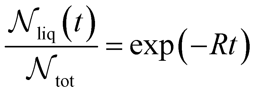 | (10) |
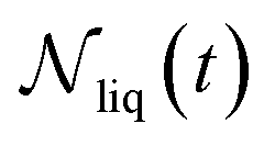 is the number of liquid droplets remaining after time t and
 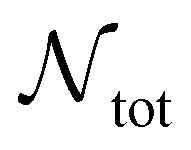 is the total number of droplets (liquid or solid) present in the experiment [equal to
 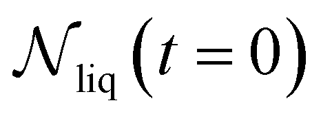 ]. In order to calculate R from continuously cooled experiments, it is necessary to divide the experiment into small time intervals Δt over which changes in temperature are treated as small. Rearranging eqn (10) we find
 | (11) |
 is the number of unfrozen droplets present at the start of the time interval and
  is the number of droplets which freeze during the time interval. We have calculated R for the three systems by treating each of their 100 replicas as a droplet. We have used Δt = 5 × 10⁻⁹ s, resulting in temperature bins 1 K wide. The results of this analysis are shown in Fig. 4c, where the data points indicate the midpoint of the temperature bins. Confidence intervals were calculated using a simple Monte Carlo simulation implemented in Stata 17.72 For physically identical droplets it is expected that the number of freezing events in a temperature interval will follow a Poisson distribution on repeat testing.71,73 For each temperature bin, the observed number of freezing events was taken as the expectation value for the bin. Poisson distributed random numbers were then generated to create 5000 simulated repeats of each of the three data sets. The bars on Fig. 4c show the 5th to 95th percentile range of the simulated experiments. (Data points generated from bins containing so few freezing events that the 5th percentile simulation had a value of R = 0 have not been included in Fig. 4c.) The freezing rates determined for the bulk system are clearly higher than those found for W = 3.5 nm. This difference is largest for the bins centered at 201.65 K, where the bulk rate is greater by approximately a factor of five.
In principle, the homogeneous nucleation rate, J, can be found as R/V where V is the volume of the water droplets undergoing freezing. Taking the volume of an mW water molecule in the liquid phase as 1/ ≈ 3 × 10⁻²⁹ m3 we find that 6000 water molecules occupy 1.8 × 10⁻²⁵ m3. Dividing our calculated freezing rates by this volume we obtain values of J entirely consistent with previous literature values29,35,63,74 for mW (see ESI†). However, obtaining J in this fashion is made possible as we know the exact number of water molecules used in our simulations. Experimentally, it is infeasible to determine the volume with such precision, so the differences in rates we report are likely inconsequential in any practical setting.
4 Assessing the impact of physical boundaries
The thin water films we have investigated so far are able to provide insight into the fundamental question of how much liquid water is needed to recover bulk-like nucleation. But, the direct relevance of thin water films in coexistence with vapor to real physical scenarios is, in fact, somewhat limited; small volumes of liquid water will form droplets with high interfacial curvature, with an associated Laplace pressure. As discussed in Section 1, Li et al.27 have found that differences in ice nucleation rate in small droplets relative to bulk water can largely be accounted for by this Laplace pressure. Notwithstanding the issues discussed in Section 3 in calculating the rate in small systems, we argue that this analysis of Li et al. is in line with our finding that J(W)/J(∞) ≈ 1 once the film is thick enough to accommodate a critical nucleus. Instead of extending our studies to small droplets, then, we instead focus on a system whose direct comparison to thin water films is more apparent: water confined between two ‘inactive’ walls.A snapshot of the system we simulate is shown in Fig. 5a. To introduce confining walls, a slab comprising 9600 atoms arranged on a FCC lattice, and exposing its (111) face, is placed such that its lowermost plane of atoms is situated at z = H/2. An identical slab is then placed such that its uppermost plane of atoms is located at z = −H/2. The atoms belonging to these slabs interact with mW water molecules via a Lennard-Jones potential. The lattice constant of the slab and the parameters for the Lennard-Jones potential (see ESI†) were chosen such that the surface only promotes ice formation at temperatures below 201 K.75 As we are investigating nucleation at T = 220 K, we can consider these surfaces to be inactive to ice nucleation, and we will assume that nucleation occurs homogeneously in the interior ‘bulk-like’ region of the fluid. Between these slabs, we introduce mW water molecules such that a ‘squished cylinder’ forms that spans one of the lateral dimensions, shown in Fig. 5a. In the orthogonal lateral dimension, a slightly convex water–vapor interface forms. The presence of a curved interface implies that, unlike the thin films considered above, the pressure inside the fluid is nonzero. In the films considered, the density far from the interfaces is virtually indistinguishable from the case of the thin water film (see ESI†). Note that the amount of water included in the simulation depends on H such that the curvature of the liquid–vapor interface is approximately constant (see ESI†).
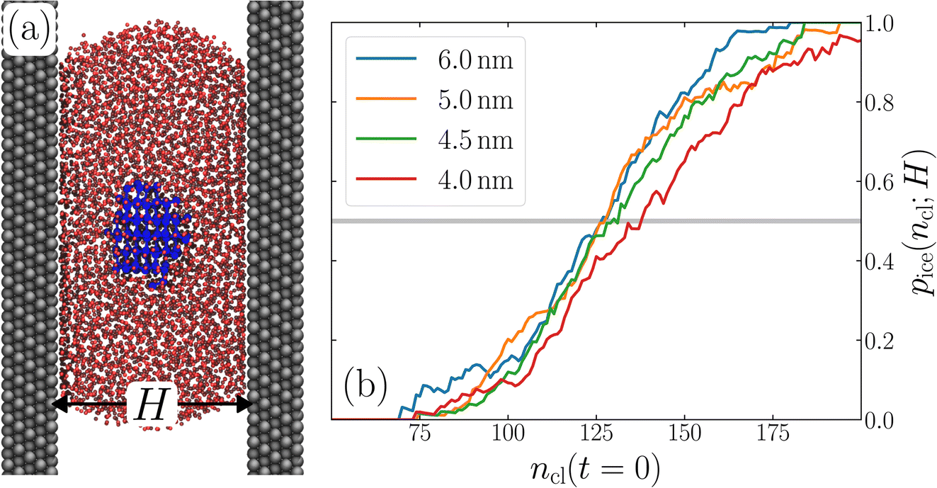 | ||
| Fig. 5 Conclusions drawn from unsupported thin films appear robust to the presence of physical boundaries. (a) Snapshot from a seeding simulation with a supported film confined between two slabs of Lennard-Jones particles separated by H = 4.5 nm. The water forms a ‘squished cylinder’ that spans the periodic boundaries of the simulation cell out of the plane of the page. In panel (b), we show pice(ncl;H), which shows that n‡cl remains bulk-like for H ≳ 4.5 nm. For H = 4 nm, the size of the critical nucleus increases, similar to what we observed in the unsupported films. | ||
Following the same procedure as we did in Section 3, we performed seeding simulations for H/nm = 4.0, 4.5, 5.0 and 6.0. In Fig. 5, we present pice(ncl; H), which shows that for H ≥ 4.5 nm, the size of the critical nucleus is insensitive to H and, within statistical uncertainty, indiscernible from n‡cl found in the thicker unsupported thin films. Also similar to the case of the unsupported films, for the smallest value of H investigated, n‡cl is seen to increase. Providing a rigorous relationship between H and W is beyond the scope of this work. Instead, in Fig. 6 we present density profiles of water for both the H = 4.5 nm confined system, and the W = 3.5 nm unsupported film (i.e., the smallest value of H and W for which n‡cl remains bulk-like). By eye, the extent of the bulk-like region in these two systems is comparable. Superposed on these plots is a snapshot (roughly to scale) of a critical nucleus for the W = 3.5 nm system, which shows that the diameter of the critical nucleus occupies the full extent of this bulk-like region. The insight gleaned from our investigation on thin films therefore also appears to hold in the more realistic case that water is confined between surfaces that do not promote ice formation.
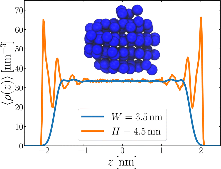 | ||
| Fig. 6 The smallest values of W (unsupported film) and H (confined between walls) for which n‡cl remains bulk-like both exhibit similar sized bulk-like regions, as seen in 〈ρ(z)〉. For the system confined between walls, 〈ρ(z)〉 is calculated such that we only consider a region far from the convex liquid/vapor interface. Overlayed on these plots is a snapshot of a critical nucleus, roughly to scale, which shows that it spans essentially all of the central bulk-like region. | ||
5 Conclusions
In this article, we have investigated ice nucleation in thin films of water, both freestanding, and confined between surfaces that do not promote ice nucleation. In both cases, our results show that the critical nucleus size is indistinguishable from that of bulk water for sample sizes that can barely accommodate its presence. At a temperature of 220 K, once the thickness is decreased below approx. 3.5 nm, we found that the size of the critical nucleus increases. These results for thin films are consistent with the observation in ref. 27 that bulk-like nucleation is recovered in nanometer sized droplets, once the Laplace pressure is taken into account, and indeed, that the rate was seen to decrease relative to that of bulk for droplets too small to accommodate a critical nucleus. Ref. 27 and this work, however, have reached this conclusion using a coarse grained representation of water interactions (the mW model), while previous work30 has found a qualitative discrepancy with a more detailed model (TIP4P/ice) when ice nucleation rates in thin films are compared to those in the homogeneous bulk. So, in this work, we have also shown that this apparent discrepancy between water models can be resolved through consistent treatment of truncated interactions between the homogeneous and inhomogeneous systems, when using more detailed models such as TIP4P/ice.In the thin film systems we have investigated, we also observed that the attachment frequencies to the critical nuclei are comparable to those in bulk water. Calculating the rate based on classical nucleation theory then gives the impression that the nucleation rate in thin films is the same as bulk water, which is seemingly at odds with some,25,29,30,33 but not all,27 previous work. A simple model that supposes nucleation is suppressed in the interfacial regions, is able to reconcile these differences at a qualitative level, but drawing quantitative conclusions on the rate (per unit volume per unit time) is made challenging by the sensitivity of the effective rate to the definition of the interfacial thickness. One scenario where one might be interested in the kinetics of ice formation under confinement is in the presence of pores or microstructures presented by solid particles such as silicas or feldspars i.e., pore condensation and freezing.66 Describing ice formation in these complex systems may benefit from simplified models, and to this end, the results of this work suggest CNT provides a reasonable foundation.
In any case, in experiments that investigate pore condensation and freezing, one typically measures the temperature at which ice forms rather than the nucleation rate directly. To gauge the impact on readily obtainable experimental observables, we therefore compared the fraction of frozen samples containing the same number of water molecules. Our results suggest that any difference in nucleation rate in a 3.5 nm thick film of water relative to that of a macroscopic sample is slight, and likely inconsequential for any experimental measurement that can be performed in the foreseeable future. They further suggest that the ice nucleation rate for water condensed in the pores of aerosol particles under cirrus cloud conditions will not be significantly suppressed due to the confined nature of the water in those pores.
6 Methods
Full details of the methodology are given in the ESI.† Liquid structures were initialized using the Packmol software package,76 and crystal structures with GenIce.77,78 All simulations were performed with the LAMMPS simulation package79 using the standard velocity Verlet algorithm.80 The temperature was controlled using a Nosé–Hoover thermostat81 and, where necessary, the pressure maintained with a Parrinello–Rahman barostat.82 Seeding systems were produced with the aid of the MDAnalysis software package.83,84For TIP4P/ice,38 simulations were performed in a similar manner, with electrostatic interactions computed with a particle–particle–particle–mesh Ewald method,85 with parameters chosen such that the root mean square error in the forces were a factor 105 smaller than the force between two unit charges separated by a distance of 1 Å.86 For simulations of liquid water in contact with its vapor, we set D = 0, where D is the electric displacement field along z, using the implementation described in ref. 87 and 88 (this is formally equivalent to the commonly used Yeh and Berkowitz89 method). The rigid geometry of the molecules was maintained with the RATTLE algorithm.90 Parallel tempering91,92 was employed for the TIP4P/ice(8.5) film as described in Section 2.
Steinhardt order parameters were calculated using the open-source, community-developed PLUMED library,93 version 2.8.94 Snapshots were created in VMD.95,96
Data availability
The data that supports the findings of this study and input files for the simulations, are openly available at the University of Cambridge Data Repository, https://doi.org/10.17863/CAM.96642.Author contributions
John A. Hayton: data curation (lead), formal analysis (lead), investigation (lead), methodology (lead), writing – original draft (lead), writing – review and editing (contributing). Michael B. Davies: conceptualization (contributing), supervision (contributing), writing – review and editing (contributing). Thomas F. Whale: formal analysis (contributing), writing – review and editing (contributing). Angelos Michaelides: conceptualization (contributing), writing – review and editing (contributing). Stephen J. Cox: conceptualization (lead), supervision (lead), investigation (contributing) writing – review and editing (lead).Conflicts of interest
There are no conflicts to declare.Acknowledgements
J. A. H. acknowledges studentship funding from the Engineering and Physical Sciences Research Council (EP/T517847/1). T. F. W. thanks the Leverhulme Trust and the University of Warwick for supporting an Early Career Fellowship (ECF-2018-127). S. J. C. is a Royal Society University Research Fellow (Grant No. URF\R1\211144) at the University of Cambridge.References
- W. Cantrell and A. Heymsfield, Bull. Am. Meteorol. Soc., 2005, 86, 795–808 CrossRef.
- M. Satoh, A. T. Noda, T. Seiki, Y. W. Chen, C. Kodama, Y. Yamada, N. Kuba and Y. Sato, Prog. Earth Planet. Sci., 2018, 5, 1–29 CrossRef.
- P. J. DeMott, A. J. Prenni, X. Liu, S. M. Kreidenweis, M. D. Petters, C. H. Twohy, M. S. Richardson, T. Eidhammer and D. C. Rogers, Proc. Natl. Acad. Sci. U. S. A., 2010, 107, 11217–11222 CrossRef CAS.
- C. Hoose, J. E. Kristjánsson, J. P. Chen and A. Hazra, J. Atmos. Sci., 2010, 67, 2483–2503 CrossRef.
- A. Gettelman, X. Liu, S. J. Ghan, H. Morrison, S. Park, A. J. Conley, S. A. Klein, J. Boyle, D. L. Mitchell and J. L. Li, J. Geophys. Res., 2010, 115, D18216 Search PubMed.
- A. Gettelman, X. Liu, D. Barahona, U. Lohmann and C. Chen, J. Geophys. Res., 2012, 117, 20201 CrossRef.
- A. Hudait and V. Molinero, J. Am. Chem. Soc., 2016, 138, 8958–8967 CrossRef CAS.
- H. Kiani and D. W. Sun, Trends Food Sci. Technol., 2011, 22, 407–426 CrossRef CAS.
- W. F. Rall and G. M. Fahy, Nature, 1985, 313, 573–575 CrossRef CAS PubMed.
- B. M. Reed, II International Symposium on Plant Cryopreservation, 2014, vol. 1039, pp. 41–48 Search PubMed.
- J. Gerrard, Rocks and Landforms, Springer Science & Business Media, 2012 Search PubMed.
- G. D. Ashton, River and Lake Ice Engineering, Water Resources Publication, 1986 Search PubMed.
- K. Rykaczewski, S. Anand, S. B. Subramanyam and K. K. Varanasi, Langmuir, 2013, 29, 5230–5238 CrossRef CAS PubMed.
- T. Fukasawa, M. Ando, T. Ohji and S. Kanzaki, J. Am. Ceram. Soc., 2001, 84, 230–232 CrossRef CAS.
- T. Fukasawa, Z. Y. Deng, M. Ando, T. Ohji and S. Kanzaki, J. Am. Ceram. Soc., 2002, 85, 2151–2155 CrossRef CAS.
- T. Ohji and M. Fukushima, Int. Mater. Rev., 2012, 57, 115–131 CrossRef CAS.
- M. Baker, Science, 1997, 276, 1072–1078 CrossRef CAS.
- K. Carslaw, R. Harrison and J. Kirkby, Science, 2002, 298, 1732–1737 CrossRef CAS PubMed.
- O. Boucher, D. Randall, P. Artaxo, C. Bretherton, G. Feingold, P. Forster, V.-M. Kerminen, Y. Kondo, H. Liao, U. Lohmann, et al., Climate Change 2013: the Physical Science Basis. Contribution of Working Group I to the Fifth Assessment Report of the Intergovernmental Panel on Climate Change, Cambridge University Press, 2013, pp. 571–657 Search PubMed.
- B. Kärcher and U. Lohmann, J. Geophys. Res.: Atmos., 2002, 107, 4698 Search PubMed.
- E. J. Jensen, O. B. Toon, A. Tabazadeh, G. W. Sachse, B. E. Anderson, K. R. Chan, C. W. Twohy, B. Gandrud, S. M. Aulenbach, A. Heymsfield, J. Hallett and B. Gary, Geophys. Res. Lett., 1998, 25, 1363–1366 CrossRef.
- P. J. DeMott, D. C. Rogers, S. M. Kreidenweis, Y. Chen, C. H. Twohy, D. Baumgardner, A. J. Heymsfield and K. R. Chan, Geophys. Res. Lett., 1998, 25, 1387–1390 CrossRef.
- D. C. Rogers, P. J. DeMott, S. M. Kreidenweis and Y. Chen, Geophys. Res. Lett., 1998, 25, 1383–1386 CrossRef CAS.
- P. J. DeMott, D. J. Cziczo, A. J. Prenni, D. M. Murphy, S. M. Kreidenweis, D. S. Thomson, R. Borys and D. C. Rogers, Proc. Natl. Acad. Sci. U. S. A., 2003, 100, 14655–14660 CrossRef CAS.
- L. Vrbka and P. Jungwirth, J. Phys. Chem. B, 2006, 110, 18126–18129 CrossRef CAS PubMed.
- L. Vrbka and P. Jungwirth, J. Mol. Liq., 2007, 134, 64–70 CrossRef CAS.
- T. Li, D. Donadio and G. Galli, Nat. Commun., 2013, 4, 1–6 Search PubMed.
- J. C. Johnston and V. Molinero, J. Am. Chem. Soc., 2012, 134, 6650–6659 CrossRef CAS PubMed.
- A. Haji-Akbari, R. S. DeFever, S. Sarupria and P. G. Debenedetti, Phys. Chem. Chem. Phys., 2014, 16, 25916–25927 RSC.
- A. Haji-Akbari and P. G. Debenedetti, Proc. Natl. Acad. Sci. U. S. A., 2017, 114, 3316–3321 CrossRef CAS.
- S. J. Cox, Z. Raza, S. M. Kathmann, B. Slater and A. Michaelides, Faraday Discuss., 2013, 167, 389–403 RSC.
- Y. Qiu and V. Molinero, J. Phys. Chem. Lett., 2018, 9, 5179–5182 CrossRef CAS.
- Y. Lü, X. Zhang and M. Chen, J. Phys. Chem. B, 2013, 117, 10241–10249 CrossRef.
- V. Molinero and E. B. Moore, J. Phys. Chem. B, 2009, 113, 4008–4016 CrossRef CAS.
- E. B. Moore and V. Molinero, Nature, 2011, 479, 506–508 CrossRef CAS PubMed.
- D. T. Limmer and D. Chandler, J. Chem. Phys., 2011, 135, 134503 CrossRef PubMed.
- E. B. Moore, E. De La Llave, K. Welke, D. A. Scherlis and V. Molinero, Phys. Chem. Chem. Phys., 2010, 12, 4124–4134 RSC.
- J. L. Abascal, E. Sanz, R. G. Fernández and C. Vega, J. Chem. Phys., 2005, 122, 234511 CrossRef CAS PubMed.
- Y. Bi, B. Cao and T. Li, Nat. Commun., 2017, 8, 1–7 CrossRef.
- E. Rosky, W. Cantrell, T. Li, I. Nakamura and R. A. Shaw, Molecular simulations reveal that heterogeneous ice nucleation occurs at higher temperatures in water under capillary tension, EGUsphere, 2023, vol. 2023, pp. 1–21 Search PubMed.
- R. O. David, C. Marcolli, J. Fahrni, Y. Qiu, Y. A. P. Sirkin, V. Molinero, F. Mahrt, D. Brühwiler, U. Lohmann and Z. A. Kanji, Proc. Natl. Acad. Sci. U. S. A., 2019, 116, 8184–8189 CrossRef CAS.
- P. J. Steinhardt, D. R. Nelson and M. Ronchetti, Phys. Rev. B, 1983, 28, 784 CrossRef CAS.
- T. Li, D. Donadio, G. Russo and G. Galli, Phys. Chem. Chem. Phys., 2011, 13, 19807–19813 RSC.
- W. Lechner and C. Dellago, J. Chem. Phys., 2008, 129, 114707 CrossRef PubMed.
- P. Rein ten Wolde, M. J. Ruiz-Montero and D. Frenkel, J. Chem. Phys., 1996, 104, 9932–9947 CrossRef.
- D. Atherton, A. Michaelides and S. J. Cox, J. Chem. Phys., 2022, 156, 164501 CrossRef CAS PubMed.
- V. Bianco, P. M. D. Hijes, C. P. Lamas, E. Sanz and C. Vega, Phys. Rev. Lett., 2021, 126, 15704 CrossRef CAS.
- J. S. Rowlinson and B. Widom, Molecular Theory of Capillarity, Clarendon Press, 1982 Search PubMed.
- X. M. Bai and M. Li, J. Chem. Phys., 2005, 122, 224510 CrossRef PubMed.
- X. M. Bai and M. Li, J. Chem. Phys., 2006, 124, 124707 CrossRef.
- E. Sanz, C. Vega, J. R. Espinosa, R. Caballero-Bernal, J. L. Abascal and C. Valeriani, J. Am. Chem. Soc., 2013, 135, 15008–15017 CrossRef CAS.
- J. R. Espinosa, C. Vega, C. Valeriani and E. Sanz, J. Chem. Phys., 2016, 144, 034501 CrossRef.
- A. Zaragoza, M. M. Conde, J. R. Espinosa, C. Valeriani, C. Vega and E. Sanz, J. Chem. Phys., 2015, 143, 134504 CrossRef PubMed.
- J. R. Espinosa, E. Sanz, C. Valeriani and C. Vega, J. Chem. Phys., 2014, 141, 18C529 CrossRef CAS.
- J. R. Espinosa, C. Navarro, E. Sanz, C. Valeriani and C. Vega, J. Chem. Phys., 2016, 145, 211922 CrossRef CAS.
- J. R. Espinosa, A. Zaragoza, P. Rosales-Pelaez, C. Navarro, C. Valeriani, C. Vega and E. Sanz, Phys. Rev. Lett., 2016, 117, 135702 CrossRef PubMed.
- J. R. Espinosa, C. Vega and E. Sanz, J. Phys. Chem. C, 2018, 122, 22892–22896 CrossRef CAS.
- M. Sega, B. Fábián, G. Horvai and P. Jedlovszky, J. Phys. Chem. C, 2016, 120, 27468–27477 CrossRef CAS.
- A. Reinhardt and J. P. Doye, J. Chem. Phys., 2012, 136, 054501 CrossRef.
- L. C. Jacobson, W. Hujo and V. Molinero, J. Phys. Chem. B, 2009, 113, 10298–10307 CrossRef CAS PubMed.
- S. Auer and D. Frenkel, Nature, 2001, 409, 1020–1023 CrossRef CAS PubMed.
- S. Auer and D. Frenkel, J. Chem. Phys., 2004, 120, 3015 CrossRef CAS.
- I. Sanchez-Burgos, A. R. Tejedor, C. Vega, M. M. Conde, E. Sanz, J. Ramirez and J. R. Espinosa, J. Chem. Phys., 2022, 157, 094503 CrossRef CAS PubMed.
- L. Lupi, A. Hudait, B. Peters, M. Grünwald, R. Gotchy Mullen, A. H. Nguyen and V. Molinero, Nature, 2017, 551, 218–222 CrossRef CAS PubMed.
- A. Haji-Akbari and P. G. Debenedetti, J. Chem. Phys., 2017, 147, 060901 CrossRef.
- M. A. Holden, J. M. Campbell, F. C. Meldrum, B. J. Murray and H. K. Christenson, Proc. Natl. Acad. Sci. U. S. A., 2021, 118, e2022859118 CrossRef CAS.
- J. M. Campbell and H. K. Christenson, Phys. Rev. Lett., 2018, 120, 165701 CrossRef CAS.
- T. F. Whale, M. A. Holden, A. N. Kulak, Y. Y. Kim, F. C. Meldrum, H. K. Christenson and B. J. Murray, Phys. Chem. Chem. Phys., 2017, 19, 31186–31193 RSC.
- E. Pach and A. Verdaguer, J. Phys. Chem. C, 2019, 123, 20998–21004 CrossRef CAS.
- G. Vali, P. DeMott, O. Möhler and T. Whale, Atmos. Chem. Phys., 2015, 15, 10263–10270 CrossRef CAS.
- T. Koop, B. Luo, U. M. Biermann, P. J. Crutzen and T. Peter, J. Phys. Chem. A, 1997, 101, 1117–1133 CrossRef CAS.
- StataCorp, Stata Statistical Software, Release 17, StataCorp LLC, College Station, TX, https://www.stata.com/ Search PubMed.
- L. D. Blackman, S. Varlas, M. C. Arno, A. Fayter, M. I. Gibson and R. K. O’Reilly, ACS Macro Lett., 2017, 6, 1263–1267 CrossRef CAS PubMed.
- J. Russo, F. Romano and H. Tanaka, Nat. Mater., 2014, 13, 733–739 CrossRef CAS.
- M. B. Davies, M. Fitzner and A. Michaelides, Proc. Natl. Acad. Sci. U. S. A., 2022, 119, e2205347119 CrossRef CAS PubMed.
- L. Martínez, R. Andrade, E. G. Birgin and J. M. Martínez, J. Comput. Chem., 2009, 30, 2157–2164 CrossRef.
- M. Matsumoto, T. Yagasaki and H. Tanaka, J. Comput. Chem., 2018, 39, 61–64 CrossRef CAS PubMed.
- M. Matsumoto, T. Yagasaki and H. Tanaka, J. Chem. Inf. Model., 2021, 61, 2542–2546 CrossRef CAS.
- A. P. Thompson, H. M. Aktulga, R. Berger, D. S. Bolintineanu, W. M. Brown, P. S. Crozier, P. J. in ’t Veld, A. Kohlmeyer, S. G. Moore, T. D. Nguyen, R. Shan, M. J. Stevens, J. Tranchida, C. Trott and S. J. Plimpton, Comput. Phys. Commun., 2022, 271, 108171 CrossRef CAS.
- W. C. Swope, H. C. Andersen, P. H. Berens and K. R. Wilson, J. Chem. Phys., 1982, 76, 637–649 CrossRef CAS.
- S. Nosé, Mol. Phys., 1984, 52, 255–268 CrossRef.
- M. Parrinello and A. Rahman, J. Appl. Phys., 1981, 52, 7182–7190 CrossRef CAS.
- N. Michaud-Agrawal, E. J. Denning, T. B. Woolf and O. Beckstein, J. Comput. Chem., 2011, 32, 2319–2327 CrossRef CAS PubMed.
- R. J. Gowers, M. Linke, J. Barnoud, J. Tyler. E. Reddy, M. N. Melo, S. L. Seyler, D. Jan, D. L. Dotson, S. Buchoux, I. M. Kenney and B. Oliver, Proceedings of the 15th Python in Science Conference, 2016, pp. 98 – 105 Search PubMed.
- R. W. Hockney and J. W. Eastwood, Computer Simulation Using Particles, CRC Press, 2021 Search PubMed.
- J. Kolafa and J. W. Perram, Mol. Simul., 1992, 9, 351–368 CrossRef CAS.
- T. Sayer and S. J. Cox, Phys. Chem. Chem. Phys., 2019, 21, 14546–14555 RSC.
- S. J. Cox and M. Sprik, J. Chem. Phys., 2019, 151, 064506 CrossRef.
- I.-C. Yeh and M. L. Berkowitz, J. Chem. Phys., 1999, 111, 3155–3162 CrossRef CAS.
- H. C. Andersen, J. Comput. Phys., 1983, 52, 24–34 CrossRef CAS.
- R. H. Swendsen and J.-S. Wang, Phys. Rev. Lett., 1986, 57, 2607 CrossRef.
- D. J. Earl and M. W. Deem, Phys. Chem. Chem. Phys., 2005, 7, 3910–3916 RSC.
- M. Bonomi, G. Bussi, C. Camilloni, G. A. Tribello, P. Banáš, A. Barducci, M. Bernetti, P. G. Bolhuis, S. Bottaro, D. Branduardi, R. Capelli, P. Carloni, M. Ceriotti, A. Cesari, H. Chen, W. Chen, F. Colizzi, S. De, M. D. L. Pierre, D. Donadio, V. Drobot, B. Ensing, A. L. Ferguson, M. Filizola, J. S. Fraser, H. Fu, P. Gasparotto, F. L. Gervasio, F. Giberti, A. Gil-Ley, T. Giorgino, G. T. Heller, G. M. Hocky, M. Iannuzzi, M. Invernizzi, K. E. Jelfs, A. Jussupow, E. Kirilin, A. Laio, V. Limongelli, K. Lindorff-Larsen, T. Löhr, F. Marinelli, L. Martin-Samos, M. Masetti, R. Meyer, A. Michaelides, C. Molteni, T. Morishita, M. Nava, C. Paissoni, E. Papaleo, M. Parrinello, J. Pfaendtner, P. Piaggi, G. M. Piccini, A. Pietropaolo, F. Pietrucci, S. Pipolo, D. Provasi, D. Quigley, P. Raiteri, S. Raniolo, J. Rydzewski, M. Salvalaglio, G. C. Sosso, V. Spiwok, J. Šponer, D. W. Swenson, P. Tiwary, O. Valsson, M. Vendruscolo, G. A. Voth and A. White, Nat. Methods, 2019, 16, 670–673 CrossRef.
- G. A. Tribello, M. Bonomi, D. Branduardi, C. Camilloni and G. Bussi, Comput. Phys. Commun., 2014, 185, 604–613 CrossRef CAS.
- W. Humphrey, A. Dalke and K. Schulten, J. Mol. Graphics, 1996, 14, 33–38 CrossRef CAS.
- J. Stone, MSc thesis, Computer Science Department, University of Missouri-Rolla, 1998 Search PubMed.
Footnotes |
| † Electronic supplementary information (ESI) available. See DOI: https://doi.org/10.1039/d3fd00099k |
| ‡ There are several similar measures of local order in the literature,43–45 but the analysis we present in this section is robust to the exact choice. |
| § In rare cases where the largest nucleus recrossed 200 molecules, the lower temperature for which ncl(T) passed 200 molecules was taken. Such recrossings occurred in fewer than 1% of our simulations. |
| This journal is © The Royal Society of Chemistry 2024 |