
 Open Access Article
 This Open Access Article is licensed under a
 Creative Commons Attribution 3.0 Unported Licence
Quantifying the dominant sources influencing the 2016 particulate matter pollution episode over northern India†
Prerita
Agarwal
 *a,
David S.
Stevenson
*a and
Mathew R.
Heal
b
*a,
David S.
Stevenson
*a and
Mathew R.
Heal
b
aSchool of GeoSciences, University of Edinburgh, Crew Building, Alexander Crum Brown Road, Edinburgh, EH9 3FF, UK. E-mail: prerita.agarwal@ed.ac.uk; david.s.stevenson@ed.ac.uk
bSchool of Chemistry, University of Edinburgh, Joseph Black Building, David Brewster Road, Edinburgh, EH9 3FJ, UK
First published on 14th May 2024
Abstract
Intense episodes of fine particulate matter (PM2.5) pollution often overwhelm large areas of the Indo-Gangetic Plain (IGP) in northern India during the post-monsoon season, a time when crop residue burning is at its peak. We conduct idealised emission sensitivity experiments using the WRF-Chem model to investigate the leading causes and spatiotemporal extent of one such extreme episode from 31 Oct to 8 Nov 2016, when hourly PM2.5 levels exceeded 500 μg m−3 across much of the IGP on several days. We utilise the anthropogenic emissions from EDGARv5.0 and the latest FINNv2.5 for fire emissions and evaluate modelled and observed ambient PM2.5 and black carbon (BC) concentrations across the IGP. The model captured the PM2.5 and BC peaks during the latter half of the episode and underestimated on other days. We find that biomass burning (BB) emissions during this episode have the strongest effect across the source regions in the upper (NW) IGP, followed by Delhi (middle IGP), where it contributes 50–80% to 24 h mean PM2.5. Complete elimination of BB emissions decreases PM2.5 concentrations by 400 μg m−3 (80–90%) in the upper IGP and by 280 μg m−3 (40–80%) across the middle IGP during this episode. Contributions from the BB source to daily varying BC concentrations are 80–90%, 40–85% and 10–60% across upper, middle and lower IGP, respectively. BB emissions dominantly contribute to daily mean secondary organic aerosols (80%), primary organic aerosols (90%), dust (60%), and nitrate (50%) components of PM2.5 across the upper and middle IGP. In comparison, the anthropogenic share of these compounds was nearly one-third everywhere except across the lower IGP. The buildup of the episode across the middle IGP was facilitated by prolonged atmospheric stratification and stagnation, causing BB-derived BC and PM2.5 to be trapped in the lowest 1 km. Our work emphasises the need for rigorous policy interventions during post-monsoon to reduce agricultural crop burning, together with targeted anthropogenic emissions control across the IGP, to minimise such extreme episodes in the future.
Environmental significancePeriodic high air pollution events across northern India lead to public health emergencies and require urgent government attention. High-resolution atmospheric chemistry transport models help elucidate the spatiotemporal characteristics of aerosol chemistry and meteorology during these episodes. We demonstrate that one such extreme pollution episode during November 2016 over the wider Indo-Gangetic Plain was primarily governed by a combination of biomass burning emissions and meteorology with varying spatial and temporal contributions. The evolution of the episode across the middle IGP was facilitated by prolonged atmospheric stratification, trapping particulate matter near the ground. Controlling biomass burning emissions during the post-monsoon period is crucial for improving air quality across northern India. |
1 Introduction
Air pollution is an urgent environmental and public health crisis in India, with evidence linking it to increased risk of cardiovascular diseases, diabetes and child undernutrition.1–6 Globally, India experiences the highest health burden from PM2.5 air pollution (fine particulate matter having aerodynamic diameter < 2.5 μm).7 In particular, around 500 million people in the Indo-Gangetic Plains (IGP) are estimated to lose eight years of average life expectancy if the current particle pollution continues.7 Annual mean PM2.5 concentrations in the IGP routinely exceed by more than ten times the 2021 World Health Organisation (WHO) air quality guideline (AQG) of 5 μg m−3 whilst Delhi often experiences PM2.5 concentrations more than 15 times this value.7,8 Concentrations are highest during the recurring IGP haze pollution events (lasting typically a week) when 24 h mean PM2.5 concentrations can exceed 500 μg m−3, resulting in a public health emergency.9–11 It is crucial to investigate the factors contributing to these episodes in order to better understand why they occur and to develop preemptive evidence-based mitigation measures.Anthropogenic emissions of aerosol particles and precursor gases in India are among the highest globally, with large regional variations.12,13 During the post-monsoon to winter period (October–February), the dominant contribution to average PM2.5 levels is from the carbonaceous particle emissions sources (such as residential biofuel combustion and agricultural biomass burning), which can contribute 60–80% to PM2.5 concentrations over northern India.14 From 2010 to 2015, due to cleaner fuel policies implemented in India, the emissions of black carbon (BC) and organic carbon (OC) from residential and informal sectors were reduced, whereas the seasonal contribution from agricultural burning continued to increase.12,13
The seasonal paddy residue burning during October–November (post-monsoon season) in the northwestern IGP plays a critical role in the severity of the air pollution episodes across the entire region.15–17 The practice of crop residue or stubble burning for clearing lands is mainly prevalent across the states of Punjab, Haryana, and western Uttar Pradesh (Fig. 1).18,19 Punjab and Haryana are the dominant contributors to India's rice and wheat stock and have witnessed an increase in crop production in the last four decades.20 A recent study has suggested a 60% increase in post-harvest fire-burning activities in the northwestern region from 2002 to 2016 was responsible for a 43% increase in aerosol burden over the IGP.21 These seasonal fires cumulatively emit substantial amounts of reactive trace gases, such as carbon monoxide (CO), oxides of nitrogen (NOx), non-methane volatile organic compounds (NMVOCs), as well as particulate matter, which are estimated to be 20 times greater than other sources of anthropogenic emissions during October–November over the NW IGP.22 A high contribution of biomass burning to ambient BC concentrations across Delhi (>40% during the high pollution days) has been reported.16,23 However, current global emissions inventories appear to underestimate biomass burning emissions, resulting in under-predictions by models of their contribution to the adverse air quality over India.24–26
 | ||
| Fig. 1 (a) Model domain showing the day and night active fire counts (red dots) detected by the VIIRS 375 m sensor between 15 Oct and 30 Nov 2016 (source: FIRMS) with terrain height (km) as the background. The white boundary represents the Indian IGP region, with the coloured rectangles showing upper (yellow), middle (orange) and lower (red) IGP sub-regions defined in this study. (b) Locations of meteorological (ASOS and radiosonde) and air quality (CPCB (PM2.5), AERONET (AOD), IMD (BC)) observation sites used for model evaluation. The shaded area represents the Indian IGP (same as the white boundary in (a)), and the inset figure is a map of the Delhi region. (c) Modelled surface PM2.5 averaged over the severe pollution episode between 31 Oct and 8 Nov 2016, with filled overlaid circles showing ground measurements averaged over the same period. (d) As (c) but for modelled BC. | ||
Here, we use the regional WRF-Chem model to quantify the dominant emissions sources driving the 2016 severe pollution episode across the IGP with a focus on the Delhi capital region, where hourly PM2.5 concentrations exceeded 1000 μg m−3 between 31 Oct and 8 Nov.9,10,15 Studies quantifying the total number of agricultural fires using satellite data during the post-monsoon period find a larger number of fires in 2016 in comparison to the last ten years.21,27–29 Despite regulatory efforts to prohibit the burning of crop residue in northwestern India and policy interventions at state levels to regulate vehicular emissions in Delhi, the post-monsoon air quality over Delhi and elsewhere has not improved in recent years, as evidenced by increased incidences of similar intense episodes.23,30–32 Studies focusing on modelling the impacts of fire emissions on the air quality during the post-monsoon period have either qualitatively analysed the impacts or have largely focused on the Delhi region.25,33 Dekker et al.34 studied the contribution of various emissions sources to carbon monoxide (CO) pollution and found residential and commercial combustion to be the dominant cause of high CO levels across the IGP during the 2017 Nov high-pollution episode. However, all these modelling studies report fire emissions to be underestimated from the respective inventories they utilised. This highlights a couple of missing pieces of information, such as a quantitative estimate of the exact cause of the 2016 episode is highly limited, together with a complete spatial investigation of particulate matter pollution using improved fire emissions (counting small fires), which is a crucial element for understanding the effects of overall pollution during this period.
We focus on quantifying contributions from anthropogenic and biomass burning sources to ambient PM2.5 and BC concentrations across the IGP during the 2016 pollution episode. (Throughout the remainder of the paper, our use of the term ‘anthropogenic’ means excluding agricultural waste burning.) We use the most up-to-date anthropogenic and fire emissions estimates and perform a series of idealised sensitivity experiments to explore the influence of each source on the spatial distribution of PM2.5 and its components with a focus on BC across the IGP. We also quantify the contribution of natural emissions during the pollution episode and examine the atmospheric stability and vertical distribution of aerosols during this episode.
2 Data and methods
2.1 WRF-Chem model setup
We used the Weather Research and Forecasting model coupled with Chemistry (WRF-Chem v4.2.1), to model atmospheric chemistry and transport.35,36 The model domain covers the northern Indian subcontinent (20–38° N and 66–90° E) at 12 km horizontal resolution (Fig. 1) and has 33 vertical layers between the surface and a top level at 50 hPa. A detailed description of our model setup and an evaluation of its performance over the domain is provided in Agarwal et al.,10 albeit with the model driven by different anthropogenic and fire emissions. Here, we provide a summary describing the new emissions data used in this work. The initial and boundary conditions and nudging for temperatures, winds and moisture are provided every six hours using the fifth-generation European Centre for Medium-Range Weather Forecasts (ECMWF) reanalysis (ERA5) at a spatial resolution of 0.25° × 0.25°.37 Nudging is applied to all vertical levels above the planetary boundary layer (PBL). Boundary concentrations for gases and aerosols are supplied six hourly from a global simulation of MOZART-4/Goddard Earth Observing System Model version 5 (MOZART-GEOS5),38 which is also used to initialize chemical fields.Gaseous and particle chemistry are respectively described using the Model for Ozone and Related Chemical Tracers (MOZART-4) chemical mechanism38,39 and the Model for Simulating Aerosol Interactions and Chemistry (MOSAIC) 4-bin aerosol module40 without aqueous phase chemistry. The MOSAIC scheme divides the aerosol dry diameter into four discrete bins (0.039–0.156 μm, 0.156–0.625 μm, 0.625–2.5 μm and 2.5–10 μm with first three bins representing PM2.5) and accounts for chemical and microphysical processes such as nucleation, coagulation and partitioning between gaseous and aerosol phases for a range of species.40 The aerosol species in MOSAIC include primary organic aerosol (POA), BC, SO42− (sulfate), NH4+ (ammonium), NO3− (nitrate), chloride, sodium, SOA (secondary organic aerosols) and other unspecified inorganic species (OIN). The other inorganic mass in the OIN bin consists of all the unidentified primary species other than POA and BC and includes inert materials, trace metals, and GOCART simulated dust mass.
The aerosol mechanism includes secondary organic aerosol (SOA) formation and evolution using the simple volatility-basis-set parameterisation described by Knote et al.41,42 The MOZART-4 gas-phase chemistry mechanism includes glyoxal SOA formation from oxidation of aromatic compounds, monoterpenes and isoprene.41,43,44
Updates to the model setup compared to that used in Agarwal et al.10 include utilisation of the recently available EDGARv5.0 monthly anthropogenic emissions for 2015 (https://edgar.jrc.ec.europa.eu/index.php/dataset_ap50).45 We also use the recently released FINNv2.5 (Fire Inventory from NCAR) for fire emissions in our domain.46 The EDGARv5.0 inventory provides emissions for SO2, NOx, CO, NMVOC, NH3, PM10, PM2.5, BC and OC at 0.1° × 0.1° horizontal resolution. The NMVOC emissions are mapped to the NMVOC species in the MOZART chemical mechanism in WRF-Chem.47 The terrestrial data, meteorology and chemical boundary conditions, including emissions from different global datasets, are interpolated to the model domain resolution. Compared with the 2010 EDGAR-HTAPv2.2 emissions, EDGARv5.0 incorporates updates in technologies, emissions factors and activity data for the energy sector based on the energy balance statistics of IEA, 2017 (ref. 48) and spatial proxies to distribute population-related emissions for 26 anthropogenic sectors. A simple day/night diurnal profile is applied to all the anthropogenic emission sectors for all the pollutants, switching between 05:30 and 17:30 local time.
As the EDGARv5.0 data incorporates agricultural waste-burning, we removed this sector from the anthropogenic emissions and utilised the FINNv2.5 data for these emissions over our domain. The FINNv2.5 emissions are available at 1 km spatial and hourly temporal resolution and provide improved detection of small fires, such as from crop residue burning, which is a major source in India post-monsoon. These small fires are reported to be underestimated in most previous inventories for India.25,33,49,50 Fig. S1† compares the daily mean anthropogenic and fire PM2.5 emissions between this and our previous study.10 The EDGARv5 emissions show higher daily average emissions over the localised hotspots of anthropogenic PM2.5 emissions compared to EDGAR-HTAPv2.2 estimates. The FINNv2.5 daily mean PM2.5 fire emissions data have totals that are nearly an order of magnitude higher than the FINNv1.5 emissions over most of Punjab and Haryana states.
Biogenic emissions are calculated online using the Model of Emissions of Gases and Aerosol from Nature (MEGAN).51 Dust emissions are also generated online using the Goddard Global Ozone Chemistry Aerosol Radiation and Transport (GOCART) scheme coupled to MOSAIC chemistry.52–54 The GOCART mechanism uses wind velocity, erosion data, vegetation type and soil moisture to calculate the dust emission flux and uses a threshold wind velocity to determine the occurrence of dust emission.53 The dust generated by GOCART is assigned to the OIN bin in the MOSAIC scheme, with 1% of the dust emitted into the first three PM2.5 size bins and 69% to the fourth (coarse) bin. The remaining dust generated by GOCART is assumed to be bigger than 10 μm diameter and to have shorter atmospheric lifetimes,53 and is ignored in the GOCART/MOSIAC module. Dust is a major contributor to total PM2.5 mass over the IGP,10,27,49 while the biogenic emissions make a small contribution during the post-monsoon season across most of the IGP.55
2.2 Sensitivity experiments and source attribution analysis
We run the simulations summarised in Table 1 for the period 27 Oct–10 Nov 2016, in order to focus on the sources and evolution of the extreme PM2.5 pollution episode over the IGP. We discard the first two days as spin-up. This period includes the Diwali festival celebrations that occurred on 30 and 31 October in 2016. Our base simulation (Base-WF) is used to evaluate the model (Section 3.1), considering it to be our best representation of the true atmospheric conditions. We further simulate three sensitivity cases (Table 1) in which all aerosol–radiation feedbacks in the model are switched off. The Base scenario is identical to the Base-WF simulation in terms of emissions, and the two further scenarios exclude either all the anthropogenic emissions (NoA) or all the fire and biomass burning emissions (NoB) in the domain. Turning the aerosol–radiation feedbacks off ensures that the Base, NoA and NoB simulations have identical meteorology so as to remove chemical responses arising from aerosol–meteorology interactions and isolate only the impacts of emissions in influencing particle pollution during the episode. This approach has been used previously in model studies quantifying the contribution of agricultural crop residue burning to air pollution in the IGP during the post-monsoon period25,56,57 as well as in other regions.58 We note that the approach of switching off all emissions of one type is an imperfect method of attribution, as there will be some non-linearities in the physico-chemical processes, particularly relating to the formation and removal of secondary pollutants. We make the assumption that these effects are generally minor across the IGP region (see later discussion).| Experiment name | Aerosol–meteorology interactions | Anthropogenic emissions | Biomass burning emissions | Natural emissions |
|---|---|---|---|---|
| Base-WF | + | + | + | + |
| Base | + | + | + | |
| NoA | + | + | ||
| NoB | + | + |
We separate the contributions to modelled PM2.5 from natural emissions and from anthropogenic and biomass burning emissions as follows. The concentrations C of a species (e.g. dust, BC, PM2.5) attributable to a particular emissions source (anthropogenic (A), biomass burning (B) or natural (N)) are then derived as shown in eqn (1)–(3):
| CA = CBase − CNoA | (1) |
| CB = CBase − CNoB | (2) |
| CN = CBase − (CB + CA) | (3) |
We derive the fractional contribution F to a particular species from a particular emission source using eqn (4),
 | (4) |
2.3 Observational data
We have previously described and evaluated the seasonal (September–November) performance of the WRF-Chem model over the IGP against multiple observation and satellite datasets.10 Here, we briefly describe the observations utilised for model evaluation of the extreme pollution episode. We also define three IGP sub-regions – upper, middle and lower (see Fig. 1) – and group the measurement locations accordingly (Table S1†).Hourly simulated surface (2 m) air temperature (T2), relative humidity (RH), wind speed (WS) and wind direction (WD) are compared with observations from the IEM-ASOS (Iowa Environmental Mesonet-Automated Surface Observing System) network. We compare model vertical meteorological profiles with observational data from the radiosonde network (RAOB), available each day at 00:00 and 12:00 UTC (05:30 and 17:30 Indian Standard Time (IST)). The stations in our IGP regions with complete sounding profiles during the study period are Delhi (77.2° E, 28.6° N, middle IGP) and Lucknow (80.9° E, 26.8° N, lower IGP).
Surface hourly PM2.5 concentrations from beta-ray attenuation instruments at 12 locations in the IGP were obtained from the Central Pollution Control Board of India (CPCB), downloaded via the OpenAQ platform. Following Kumar et al.59 we removed highly suspect data (e.g., sampled values > 1500 μg m−3 and consecutive hourly values equal to 985 μg m−3). Surface hourly BC measurements at 4 sites, mostly representing urban clusters in the IGP, were obtained from the India Meteorological Department (IMD) network. The BC concentrations are derived from an AE-33 Aethalometer as described in Kumar et al.60 We also compared modelled and observed aerosol optical depth at 550 nm (AOD550 nm) retrieved from the ground-based Aerosol Robotic Network (AERONET)61 and from MODIS sensors on board the Terra and Aqua polar orbiting satellites. Only the Kanpur (lower IGP) and Lahore (upper IGP) AERONET locations have sufficient data during our study period. Modelled AOD is compared for the same time as the sampled local satellite overpass times of 10.30 (Terra) and 13.30 (Aqua).
We use mean bias (MB), normalized mean bias (NMB), mean absolute error (MAE), root mean square error (RMSE) and Pearson's correlation coefficient (r) as statistical metrics for reporting the model's performance.
3 Results and discussion
3.1 Model characterisation of the severe pollution episode
Extensive model evaluation in simulating seasonal monsoon to post-monsoon meteorology and air quality over the full domain was reported in our previous work.10 Here, we focus on the spatiotemporal evolution of the severe pollution event over the upper, middle and lower IGP sub-regions in the Base-WF simulation. The Base-WF and Base configurations predict the overall trends in meteorology and aerosol chemistry similarly and doesn't change our results for the source attribution investigation. The overall modelled daily and diurnal meteorology trends for T2, RH, and wind patterns show a good agreement with the observations and capture observed variations very closely across the middle and lower IGP. However, the WS are overestimated almost everywhere by 1–1.5 m s−1. A more detailed comparison of observed and simulated meteorological variables is provided in Section S1;† here, we focus on evaluating PM2.5, BC and AOD.Fig. 2 shows the comparison of the time series of modelled surface PM2.5 and BC concentrations against the observations averaged over the available sites in the three IGP regions. The simulated concentrations are considerably enhanced compared to our earlier results10 due to the updated emissions inputs. During the episode, observed PM2.5 concentrations averaged across upper, middle and lower IGP measurement locations were 112 μg m−3, 417 μg m−3, and 219 μg m−3, respectively, and modelled PM2.5 concentrations were 86 μg m−3, 283 μg m−3, and 130 μg m−3. The model reproduces the daily PM2.5 concentrations trend across the upper IGP quite well. However, the measurement sites in the upper IGP for PM2.5 (Panchkula & Mohali) and BC (Chandigarh) are northeast of the main open biomass burning activities (Fig. 1) which limits assessment of the model's performance in simulating the variability in surface pollution over the region with greatest fire activities. It is, therefore, crucial to monitor air quality in the biomass-burning source regions of NW India, in addition to in the major cities, as was also emphasised by Singh et al.62
 | ||
| Fig. 2 Comparison of modelled (red) and observed (black) hourly mean concentrations of PM2.5 (left) and BC (right) averaged across the network of ground measurement sites (CPCB, IMD respectively) in the upper, middle and lower IGP regions. The vertical dashed lines in each panel delineate the pollution episode, and the r values are the Pearson's correlation coefficients. | ||
The start of the pollution episode around Oct 31 is evident everywhere from the observed PM2.5 and BC concentration peaks (600–800 μg m−3 and 20–90 μg m−3, respectively). The beginning of the episode is less distinct in the modelled BC and PM2.5 time series compared with the observed values. This is likely due to the localised emissions from the Diwali festival (associated with widespread firecracker activities between 30 and 31 Oct), which are not included in the emissions inventory. The model struggles to reproduce the PM2.5 and BC peaks in the first half of the episode (due to low bias) across middle and lower IGP regions and comes close to capturing the peaks in the latter half. Particularly over the middle IGP region, the model underestimates the peaks in PM2.5 by more than 500 μg m−3 on 2 and 4 Nov and overestimates the peaks by nearly 400 μg m−3 on 5 and 8 Nov. The overall daily PM2.5 variability is fairly well reproduced by the model across the upper IGP and generally underestimated elsewhere across the IGP. Compared to the other regions, the daily measured BC concentrations across the middle IGP are generally higher and peak on 31 Oct (exceeding 90 μg m−3). The model underestimates the BC concentrations everywhere by 55–82% on average (Table S3†), except during the middle of the episode when it accurately predicts some of the observed peaks across the middle IGP. The diurnal features in the modelled PM2.5 and BC concentration show night-time maxima and daytime minima, approximately capturing the observed trends. The magnitude of the diurnal cycle is generally smaller in the model, with a better representation of low mid-day values than the high night-time values.
Consequently, the modelled PM2.5 averaged over the whole episode shows an overall negative mean bias ranging from −25 to −134 μg m−3 and an RMSE in the range of 63 to 259 μg m−3 across the three IGP regions (Table S3†). The model generally captures some of the observed BC peaks across the middle IGP, synchronous with PM2.5. During the episode, the calm winds (less than 1 m s−1), which generally blew from the west and northwest direction, led to the accumulation of transported and locally emitted air pollutants over Delhi. A marked increase in surface wind speeds by about 2–4 m s−1 drove the gradual dispersion of pollutants by 8 Nov. Notably, the surface BC concentrations observed over Delhi during this event exceeded those reported during severe haze episodes over the Beijing metropolis by nearly a factor of three.63,64
Modelled AOD550 nm is also compared against the AERONET observations at the Lahore and Kanpur sites in the upper and lower IGP, respectively (Fig. S4†). The observed AOD over Lahore, which is close to but upwind of the fire activity region, reached as high as 4.2 on 2 Nov and averaged greater than 2.0 throughout the episode. This steep gradient in observed AOD over Lahore likely indicates a possible error in the modelled biomass burning plume drifting further from the fire region to downwind areas, resulting in a dramatic decrease after 30 Oct over Lahore. The model is strongly biased low for Lahore but compares better over Kanpur, where the correlation coefficient (r) is 0.66.
To obtain a better understanding of the spatial features of this widespread severe episode, we also compare in Fig. 3 the spatial distribution of modelled and MODIS retrieved AOD550 nm. The model predicts the spatial distribution of AOD across the domain quite well (spatial correlation, r = 0.78). It, however, fails to capture the extremely high AOD values (≈3.0) across localised areas in the southern parts of the NW IGP states (Fig. 1) and underestimates AOD here by a factor of 2. Both model and satellite maps show the upper IGP and neighbouring areas to exhibit the highest AOD values.
 | ||
| Fig. 3 Modelled and MODIS retrieved AOD550nm sampled at overpass times of 10.30 (Terra) and 13.30 (Aqua) and averaged over the pollution episode. The right panel shows the absolute differences between the model and satellite values (with a % difference plot shown in Fig. S6†), and r is the Pearson's correlation coefficient. | ||
Despite utilising the latest EDGARv5 anthropogenic emissions and FINNv2.5 fire emissions, the modelled PM2.5 and BC concentrations and AOD values are overall biased low during this episode. Likely reasons for this include missing episodic local emissions (e.g., festive firecrackers), underestimation of primary aerosol emissions in the inventories (e.g. BC and POA), overestimated dilution of pollutants, and limited measurement sites for model-observations comparisons, as well as the exceptional nature of the pollution event itself. Additionally, the absence in the input emissions of hydrogen chloride (HCl) gas emissions from local rubbish and crop residue burning, which yield high chloride aerosol concentrations in parts of Delhi post-monsoon,23,65 may also contribute to PM2.5 underestimation. However, although the evaluation indicates the model is not entirely precise at simulating PM2.5 and BC concentrations, attribution results in the following sections should be interpreted in the wider context of the model being able to simulate the total PM2.5 and BC approximately. Despite the model biases and uncertainties, we believe that the attribution results are a useful indication of the importance of different sources.
3.2 Contributions of emissions sources to daily PM2.5 and its components and to BC
Fig. 4 shows the modelled fractional contributions of anthropogenic, biomass burning (BB) and natural dust emissions to daily surface PM2.5 (i.e. F(PM2.5)A, F(PM2.5)B and F(PM2.5)N) and BC in the three IGP regions for each day of the episode. In the upper and middle IGP regions, the BB source is the dominant contributor to the high modelled PM2.5 and BC concentrations, with a daily fractional contribution varying between 0.4 and 0.85. In the upper IGP, daily F(PM2.5)B is greater than 0.75 throughout the episode. In the middle IGP, daily F(PM2.5)B increases from 0.4 to 0.87 after 2 Nov, and in the lower IGP, F(PM2.5)B similarly increases from 0.3 to 0.7 from 5 Nov. This indicates that the contribution of BB to PM2.5 is greatest across the source regions in the NW IGP, with the middle and lower IGP subject to substantial transport of BB-derived PM2.5 a few days later. | ||
| Fig. 4 Fractional contributions of biomass burning, natural and anthropogenic emissions to daily mean modelled surface PM2.5 (left panels) and BC (right panels) averaged over the upper, middle and lower IGP regions shown in Fig. 1 for each day of the extreme pollution event (31 Oct–8 Nov 2016). | ||
Similar trends appear for the BB contribution to BC over these regions. In the upper IGP, nearly all BC during the episode derives from BB, with F(BC)B ranging from 0.8 to 0.9. In the middle and lower IGP, daily F(BC)B is in the ranges 0.2–0.8 and 0.1–0.5, respectively. This is consistent with the typical regional downwind dispersal of the episodic post-monsoon aerosol across the IGP by the prevailing meteorology.10,59,66 The fractional contribution of natural emissions to PM2.5 is mostly less than 0.1 throughout the episode everywhere in IGP.
Fig. 5 shows the relative contributions of BB and anthropogenic sources to the individual chemical components of modelled daily PM2.5 concentrations for each region during the episode. The daily variations apparent in the C(PM2.5)A components are controlled by meteorology, as the anthropogenic emissions in the model do not vary from day to day during this period. Nitrate (NO3−) and secondary organic aerosols (SOA) from anthropogenic sources account for 0.5–0.7 of the C(PM2.5)A across all the IGP regions, followed by dust (OIN), ammonium (NH4+) and sulfate (SO42−) aerosols. Although the hourly varying BB emissions are highly localised to the NW states, the daily variation in C(PM2.5)B across the middle and lower IGP shows a gradual increase during the latter half of the episode, owing to shifts in the regional distribution and increased fire activity in NW on those days (Fig. S5†). In addition to contributing large concentrations of primary organic aerosols (POA; ≈90%), BB emissions are responsible for an additional 100–120 μg m−3 and 50–200 μg m−3 of SOA across upper and middle IGP, respectively. On average, the next two largest BB-originated PM2.5 components across these two regions are OIN and NO3− each ranging between 10 and 100 μg m−3. However, BB emissions have a negligible contribution to sulfate aerosols everywhere. Nitrate is a dominant component of C(PM2.5)B and C(PM2.5)A throughout the episode, consistent with post-monsoon measurement studies.65,67 The C(BC)B vary between 30–35 μg m−3 and 10–25 μg m−3 across upper and middle regions, respectively. Across the lower IGP, anthropogenic emissions dominate the contributions to daily PM2.5 during the first half of the episode, whilst during the second half, BB emissions make comparable contributions to daily PM2.5.
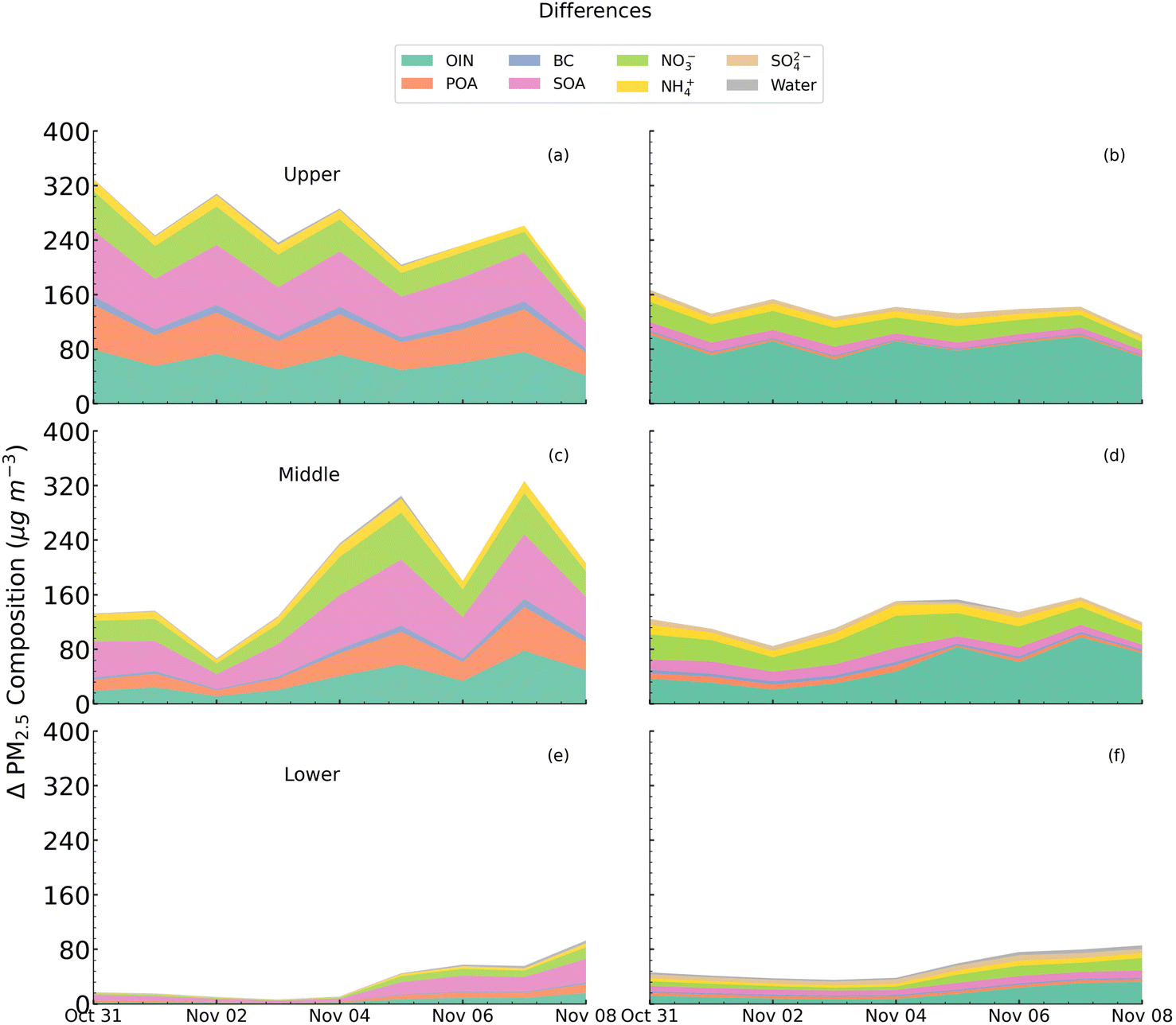 | ||
| Fig. 5 Absolute contributions of biomass burning emissions (a, c and e) and anthropogenic emissions (b, d and f) to the different chemical components of daily mean modelled PM2.5 concentrations averaged over the upper, middle and lower IGP regions shown in Fig. 1 for each day of the extreme pollution event (31 Oct–8 Nov 2016). The individual species abbreviations are: OIN (other inorganics or dust) SOA (secondary organic aerosols), POA (primary organic aerosol), SO42− (sulfate), NH4+ (ammonium), NO3− (nitrate), BC (black carbon). | ||
Overall, it is evident that the extreme pollution episode of November 2016 across northern India was dominated by episodic BB emissions, which, in addition to the direct contribution of POA, also contributed to the sustained build-up of secondary organic and inorganic aerosols. The increased F(PM2.5)B together with the more realistic simulation of total PM2.5 in the second half of the episode, likely suggests that some of the errors with underestimating PM2.5 in the first half of the episode are related to the BB fraction being underestimated. In terms of total PM2.5 concentrations, even without the seasonal BB source, the daily mean PM2.5 still exceeds the 24 h WHO AQG of 15 μg m−3 by 6–7 times over the Delhi capital region and exceeds the Indian National Ambient Air Quality Standards (NAAQS) of 60 μg m−3 by 40–60 μg m−3. Across the upper IGP, the daily mean PM2.5 concentrations would be about five times the 24 h WHO AQG and 10–20 μg m−3 higher than the NAAQS recommendation in the absence of the BB emissions, while daily mean PM2.5 across lower IGP generally would remain within the NAAQS value.
3.3 Spatially varying sensitivity of PM2.5 and BC concentrations to source emissions
Fig. 6 shows the distribution of the episode averaged surface PM2.5 concentrations across the whole domain and the relative contribution from each source to its spatial distribution. Across the northwest, BB emissions from the central and southern edges of the states of Punjab and Haryana (where agricultural fire activities are greatest, see Fig. 1 and S1†) contribute ≈400 μg m−3 (80–90%) to the episode mean PM2.5. Even in densely populated Delhi in the middle IGP (with negligible fires), as much as 60–70% (≈250 μg m−3) of the PM2.5 originates from non-local BB emissions. This further demonstrates the influence of downwind transport to Delhi from the BB source regions. These findings are consistent with Kulkarni et al.,25 who reported a 50–75% contribution from crop residue fires to modelled PM2.5 levels in Delhi in the 2018 post-monsoon period. However, BB emissions do not play such a dominant role in the rest of the domain, where F(PM2.5)A is approximately 0.6. In terms of relative spatial share, the F(PM2.5)B of ≈0.9 in the upper NW region is almost an order of magnitude higher than in the eastern parts of the domain, where F(PM2.5)A is predominant. As a consequence, substantial reductions in episodic PM2.5 concentrations (50–85%) are simulated across the IGP when seasonal BB emissions are removed from the domain. | ||
| Fig. 6 Spatial contributions of natural, anthropogenic and biomass-burning emissions to surface PM2.5 concentrations averaged over the extreme pollution episode. The top panel shows the mean PM2.5 concentrations, while the middle and bottom row respectively demonstrates the absolute (C(PM2.5)N, C(PM2.5)A, C(PM2.5)B) and fractional (F(PM2.5)N, F(PM2.5)A, F(PM2.5)B) contributions to PM2.5 from the three emission sources. The values of F less than 0 and more than 1 in the bottom panel are shown as white and dark blue in the colour scale. | ||
The contribution of F(PM2.5)N is less than 0.1 (≤30 μg m−3) relative to the anthropogenic and BB sources across NW, central and eastern regions of the domain, but almost entirely dominates over the less populated arid regions in the west and north (Fig. 6). The F(PM2.5)A over this arid region shows a contrasting behaviour compared to other aerosols. Over here, the source attribution method simulates, however, a rather nonlinear relationship between F(PM2.5)N and anthropogenic emission source that gives rise to different chemical regime in this part of the domain. The explanation for this requires an improved understanding of the chemical processes involving dust particles, which is the subject of our companion paper focusing on dust aerosols over the desert region. The non-linear chemistry in the model may also affect other aerosol components in other parts of the domain, the manifestation of which may be precluded by the 100% emissions-off approach of idealised emissions sensitivity scenarios. Moreover, our current findings suggest that even the complete elimination of anthropogenic emissions may elicit varying responses across different regions, and hence a need to understand these mechanisms using chemical transport models.
Fig. 7 illustrates a similar spatial analysis of emissions contribution as Fig. 6 but for surface BC concentrations. (Natural emissions do not contribute to BC, so this source is not shown in these maps.) As for PM2.5, BC concentrations are strongly dominated by F(BC)B across upper IGP (0.9), followed by middle (0.45) and lower (0.3) regions. Fig. 7 also reveals other localised hotspots across dense urban and industrialised areas where C(BC)A dominates. However, across Delhi, the average F(BC)A contribution is slightly higher (0.6–0.7) than F(BC)B. This demonstrates the share of localised C(BC)A over the Delhi region (from road transport and cooking) is almost comparable to the regionally transported and episodic C(BC)B. These modelled contributions of BC from BB across Delhi agree well with the measurement work of Bikkina et al.,16 who showed, using dual-carbon isotopes, that ≈42 ± 17% of BC derived from crop residue/biofuel burning during the post-monsoon season. Anthropogenic contributions to BC are also generally dominant in the remainder of the domain, such as in eastern and central India and parts of Pakistan in the west.
 | ||
| Fig. 7 Same as Fig. 6, but for surface BC concentrations. Natural dust emissions do not contribute to BC, so this source is not included in the maps. | ||
3.4 Implications of atmospheric stability on the vertical distribution of pollutants
Several studies have attributed the 2016 post-monsoon extreme pollution episode across Delhi and lower IGP to the prevailing stagnant conditions in addition to episodic local and regional emissions.9,34,68,69 While the objective of this section is to examine the role of meteorological stability in driving severe pollution events, it is valuable to compare the sounding observations with the model to demonstrate its ability to capture the basic features of the upper air thermodynamic structure. Fig. 8 shows the model and radiosonde daily 5:30 and 17:30 local time (LT) vertical variation of temperature (°C) and WS (m s−1) during the pollution episode for Delhi and Lucknow (in the middle and lower IGP regions, respectively). The model shows close agreement with observations for both temperature and WS. The vertical temperatures show consistent temperature inversions on all days at 5:30 LT over Delhi, with dramatic decreases of about 5–6 °C from the surface to about 940 hPa aloft compared to Lucknow. The strong nocturnal inversion at 5:30 LT is associated with calm near-surface WS (0–1 m s−1) during the entire study period (31 Oct–8 Nov). Air stagnation conditions are identified by Wang and Angell,70 as being a minimum of 4 days with near-surface WS < 4 m s−1 and temperature inversions below 850 hPa. The nocturnal air stagnation state identified during this severe pollution event demonstrates the conditions highly favourable for trapping pollutants and the absence of convective and wind-driven dispersion required to dilute air pollutants.71 In contrast, the 17:30 LT vertical temperature and WS profiles at Delhi and Lucknow show a more mixed-layer atmosphere state in the evening following the heating during the day. This enables the vertical mixing of pollutants to the top of the residual mixed layer at this hour. This could well indicate a dilution of pollutants in the mixed layer during evening hours driven by convection.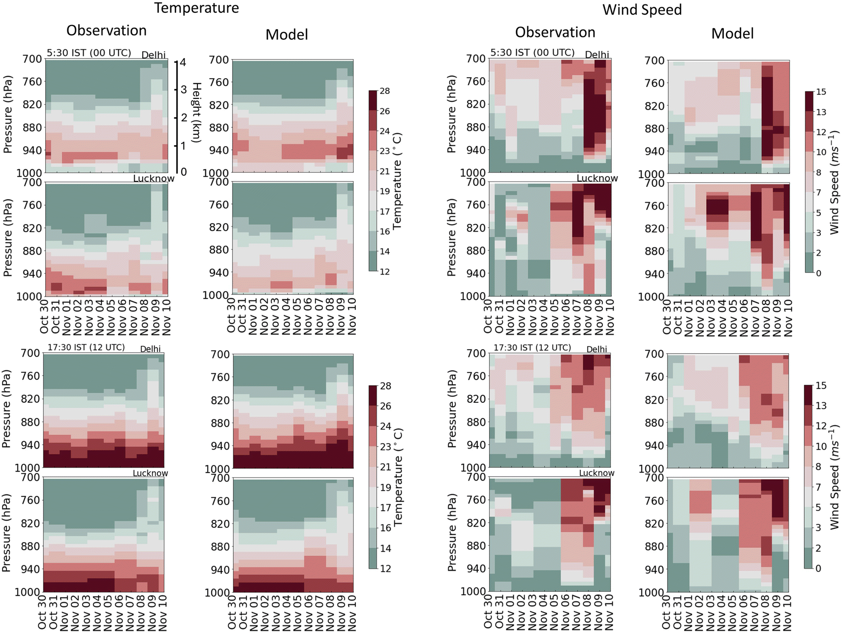 | ||
| Fig. 8 Altitudinal variation (1000 to 700 hPa) of observed and simulated temperature and wind speed (m s−1) at 5:30 LT (IST) (top panel) and 17:30 LT (bottom panels) during the pollution episode. The observations are obtained from radiosonde profiles at Delhi and Lucknow, in the middle and lower IGP regions, respectively, as shown in Fig. 1. | ||
Fig. 9 shows modelled hourly vertical profiles of the concentrations of PM2.5 and BC over Delhi derived from anthropogenic emissions and from BB emissions, together with the hourly PBLH. The C(PM2.5)B and C(BC)B concentrations show significantly increased vertical and temporal evolution compared to their anthropogenic counterparts. The obvious peaks in both PM2.5 and BC variability between 5 and 8 Nov in Fig. 2 are clearly shown by the model to be of BB origin, particularly at night-time when PBLH falls to <100 m. Sporadic peaks in C(PM2.5)B and C(BC)B show BB emissions contributions to PM2.5 and BC as high as 900 and 30 μg m−3, respectively, in the lower layers of the atmosphere (up to 1 km). On the other hand, C(PM2.5)A and C(BC)A concentration evolution shows a more pronounced diurnal behaviour, especially for BC, that remains below 100 m in vertical stratification and decreases more rapidly with altitude compared to the BB-derived concentrations. Consequently, the contribution from biomass burning emissions at this time leads to elevated pollutant distribution in the upper layers across Delhi, reaching above 1 km, as compared to anthropogenic emissions. Since our sensitivity model configuration does not include aerosol–radiation interactions so as to provide identical meteorology in each experiment, the particle pollution dynamics here are controlled by emissions and meteorology.
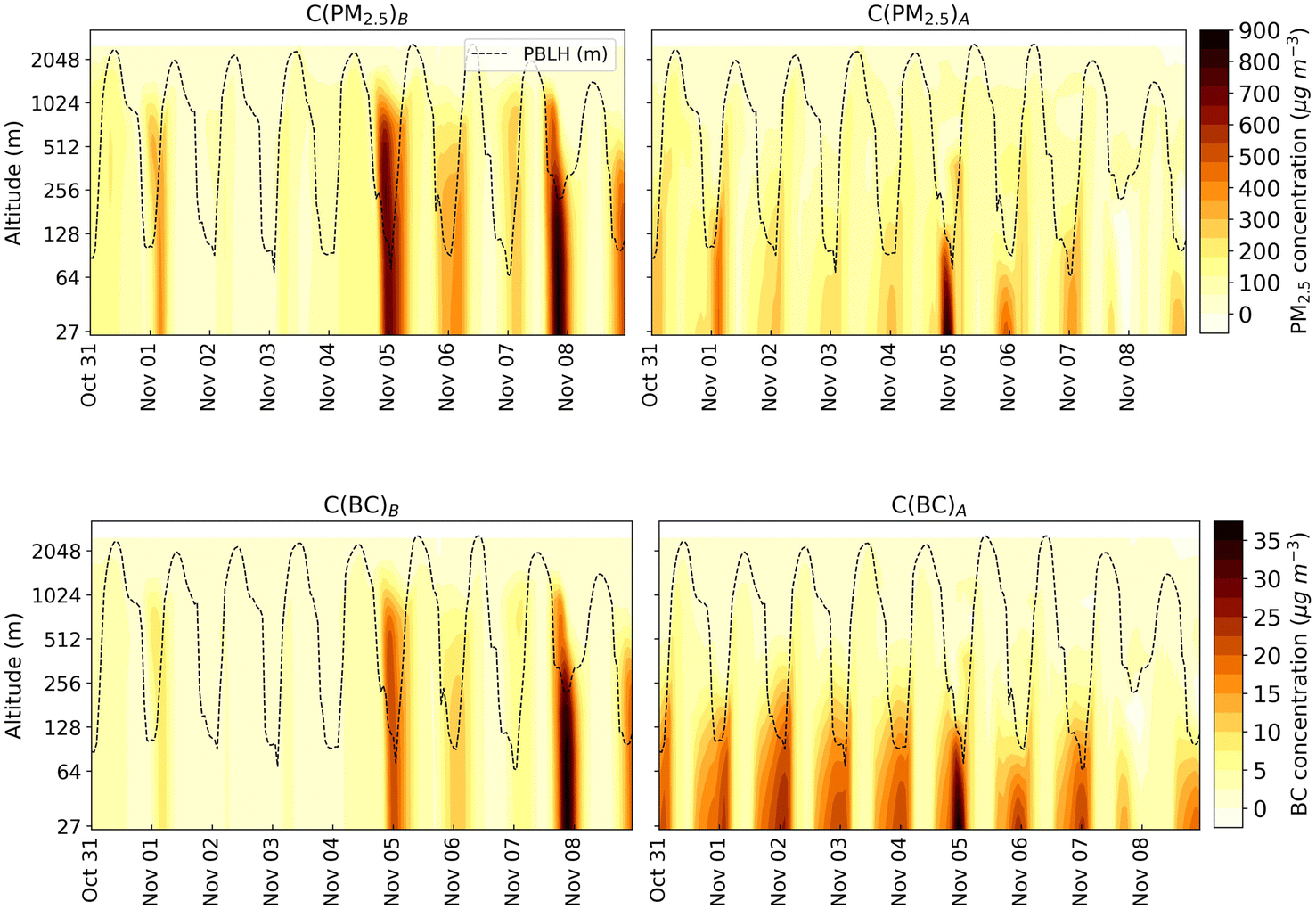 | ||
| Fig. 9 Modelled vertical evolution of changes in total PM2.5 (top) and BC (bottom) concentrations over Delhi due to the exclusion of anthropogenic and BB emissions as compared to the Base scenario during the study period. The dashed line in the top panels denotes the hourly variation of the modelled planetary boundary layer (PBL) height (identical in all sensitivity runs). | ||
3.5 Limitations
Model simulation of this (and similar) extreme PM pollution episodes is inherently challenging because these events are driven, at least in part, by strong transient local emissions that are not captured as model input. This shortcoming is reflected by the model negative bias reported here for PM2.5 and BC during the extreme PM episode. The model uses the best estimates of emissions on average (e.g., for month of year, hour of the day, for a particular biomass burning event, etc.) but cannot capture highly spatially and temporally dynamic changes in emissions in reality: for example, episodic particle emissions during the Diwali festival celebrations, or from local rubbish burning. Further development of locally relevant temporal profiles for anthropogenic emissions is needed, with simulations performed at finer spatial resolution than the present model (12 km) to capture these crucial local features during a haze episode. As noted in Section 3.1, the model also does not currently incorporate chloride particles formed from HCl emissions from local rubbish and crop residue burning that have been observed to contribute significant PM concentration in post-monsoon Delhi. This is an area of future model development.A further potential contributor to the underestimation of surface PM in this work is a small model positive bias for surface windspeed and the potential influence of BC radiative effect on boundary-layer depth. On the other hand, there is evidence that the model overestimates natural dust concentrations due to both overestimation of dust uplift and underestimation of dust deposition arising from a dry bias in the model.10 As PM composition observations were lacking for this study period, the model's ability to accurately represent particle compositional chemistry remains uncertain. This work analyses the modelled SOA and SIA aerosol fractions of PM2.5, but a more detailed assessment of aqueous aerosol-phase chemistry and its sensitivities to precursor gases would be helpful in characterising the intense haze episodes. Despite these acknowledged uncertainties in absolute quantification, we expect that the model provides reliable insight into the spatio-temporal drivers of PM and its components during this episode.
4 Conclusions
The Indo-Gangetic Plain (IGP) in northern India experienced one of the worst air quality episodes during the 2016 post-monsoon season from 31 Oct to 8 Nov. In this work, the WRF-Chem model with up-to-date anthropogenic and fire emissions is applied to investigate the influence and source contribution of anthropogenic, seasonal agricultural residue burning, and natural dust emissions to this episode (where anthropogenic means excluding agricultural waste burning). The model adequately reproduces the surface meteorological features compared to observations during this period. Notably, during the severe episode, the frequency of polluted westerly and northwesterly flow (50%) increased across upper, middle and lower IGP sub-regions, highlighting the regional distribution of pollution by 8 Nov. We find that observed near-surface meteorology showed remarkably weak wind speeds (WS) during this period which restricted the dilution and mixing of pollutants and prolonged the episode. The model underestimates the PM2.5 in the initial days but captures some of the hourly peak PM2.5 concentrations (500–650 μg m−3) during the latter half of the episode. In the middle IGP region, Delhi experienced some of the highest observed and modelled PM2.5 concentrations. The observed trend of hourly BC concentration shows substantial daily variation everywhere, which the model reproduces well, but the daily peaks are mostly underestimated except over Delhi, where the model shows dramatic enhancements between 5 and 8 Nov. Our comparison shows the model underestimates AOD550 nm over these regions by a factor of 2 but captures the spatial correlation very well (r = 0.78).Our study suggests that localised biomass burning emissions contributed 50–80% of daily mean PM2.5 across the upper IGP source regions and downwind middle IGP region. Likewise, the daily varying black carbon (BC) concentrations across the upper and middle IGP regions were governed by biomass burning emissions (fractional contribution range 0.8–0.9 and 0.25–0.8, respectively), whereas in the lower IGP, anthropogenic emissions were the main driver of BC loading. The regionally distributed composition of daily mean PM2.5 during the episode reveals biomass burning contributed approximately 90% of primary organic aerosols (POA), 80% of secondary organic aerosol (SOA), 70% of dust and 50% of nitrate aerosols across the upper and middle IGP. In comparison, the anthropogenic share of these components was almost one-third everywhere except across the lower IGP. Furthermore, we show that both sources contribute comparably to the nitrate fraction of the modelled PM2.5 across upper and middle IGP. We demonstrate that a drastic reduction or complete elimination of BB emissions would substantially mitigate these extreme episodes across NW IGP, while a strategic control of anthropogenic emissions is also necessary to reach the 24 h mean NAAQS limit for PM2.5 (60 μg m−3).
The spatial PM2.5 sensitivities to emission sources show a strong north-to-south and west-to-east gradient in the domain with regionally varying non-linear responses to anthropogenic emissions. The episodic PM2.5 loading from 31 Oct to 8 Nov affected large parts of the IGP, with the NW and middle IGP experiencing the highest daily and episode average PM2.5 concentrations. The PM2.5 sensitivity to BB emissions is strongest and highly localised to the NW, where they account for nearly 80% of the total mean PM2.5 loading. Across most of the lower IGP, the mean PM2.5 from anthropogenic emissions show a considerable fraction (by nearly 90%). The BC distributions are consistent with those of PM2.5 across the IGP region and display a geographically varying response to the emissions. However, the regional responses of the BC distribution are much stronger everywhere, with over 90% of BC originating from anthropogenic sources except in the NW IGP, where contributions from biomass burning sometimes reach 95% during this episode.
Finally, we report that the exceedingly high PM2.5 and BC concentrations on some days during the episode in Delhi were also controlled by frequent nocturnal temperature inversions and atmospheric stratification in addition to regional and local pollution. The modelled biomass burning derived PM2.5 and BC show enhanced vertical distributions of as much as 900 and 30 μg m−3, respectively, up to 1 km in the atmosphere. In comparison, anthropogenic PM2.5 and BC loading remain below 0.1 km and exhibit a strong diurnality for BC. The vertical distribution of aerosol particles higher up in the atmosphere could be detrimental to increased local warming in the lower and middle troposphere, which remains a crucial and currently unexplored aspect of this episode. Understanding the impact of each source on the development of an extreme air pollution event is critical for any effective mitigation strategy. Our results show that emission sources have a varying impact on particle pollution across different regions across northern India. The pollution control strategies over most of IGP should aim to mitigate these extreme haze episodes by radically controlling the seasonal biomass burning emissions, followed by regulating the local anthropogenic sources to improve the overall air quality during the peak pollution period.
Author contributions
PA, DSS and MRH conceptualised the study. PA compiled the measurement datasets, performed formal model simulations and data analyses, curated the data and wrote the text with discussions and supervision by MRH and DSS. DSS and MRH edited and commented on the text.Conflicts of interest
The authors declare that they have no conflict of interest.Acknowledgements
PA acknowledges UoE scholarships (Principal's Career Development Scholarships and Edinburgh Global Research Scholarship). DSS acknowledges support from the Natural Environment Research Council (grant no. NE/S009019/1). We acknowledge the use of observation data for black carbon provided by VK Soni, India Meteorological Department (IMD), and quality controlled PM2.5 data for Mohali by Vinayak Sinha, Baerbel Sinha and their research group at IISER, Mohali.References
- A. J. Cohen, M. Brauer, R. Burnett, H. R. Anderson, J. Frostad, K. Estep, K. Balakrishnan, B. Brunekreef, L. Dandona, R. Dandona, V. Feigin, G. Freedman, B. Hubbell, A. Jobling, H. Kan, L. Knibbs, Y. Liu, R. Martin, L. Morawska, C. A. Pope, H. Shin, K. Straif, G. Shaddick, M. Thomas, R. v. Dingenen, A. v. Donkelaar, T. Vos, C. J. L. Murray and M. H. Forouzanfar, Lancet, 2017, 389, 1907–1918 CrossRef PubMed.
- D. Prabhakaran, P. Jeemon, M. Sharma, G. A. Roth, C. Johnson, S. Harikrishnan, R. Gupta, J. D. Pandian, N. Naik, A. Roy, R. S. Dhaliwal, D. Xavier, R. K. Kumar, N. Tandon, P. Mathur, D. K. Shukla, R. Mehrotra, K. Venugopal, G. A. Kumar, C. M. Varghese, M. Furtado, P. Muraleedharan, R. S. Abdulkader, T. Alam, R. M. Anjana, M. Arora, A. Bhansali, D. Bhardwaj, E. Bhatia, J. K. Chakma, P. Chaturvedi, E. Dutta, S. Glenn, P. C. Gupta, S. C. Johnson, T. Kaur, S. Kinra, A. Krishnan, M. Kutz, M. R. Mathur, V. Mohan, S. Mukhopadhyay, M. Nguyen, C. M. Odell, A. M. Oommen, S. Pati, M. Pletcher, K. Prasad, P. V. Rao, C. Shekhar, D. N. Sinha, P. N. Sylaja, J. S. Thakur, K. R. Thankappan, N. Thomas, S. Yadgir, C. S. Yajnik, G. Zachariah, B. Zipkin, S. S. Lim, M. Naghavi, R. Dandona, T. Vos, C. J. L. Murray, K. S. Reddy, S. Swaminathan and L. Dandona, Lancet Glob. Health, 2018, 6, e1339–e1351 CrossRef PubMed.
- L. M. David, A. R. Ravishankara, J. K. Kodros, J. R. Pierce, C. Venkataraman and P. Sadavarte, GeoHealth, 2019, 3, 2–10 CrossRef PubMed.
- WHO, WHO Global Air Quality Guidelines: Particulate Matter (PM2.5 and PM10), Ozone, Nitrogen Dioxide, Sulfur Dioxide and Carbon Monoxide, World Health Organization, 2021 Search PubMed.
- S. Mandal, S. Jaganathan, D. Kondal, J. D. Schwartz, N. Tandon, V. Mohan, D. Prabhakaran and K. M. V. Narayan, BMJ Open Diabetes Res. Care, 2023, 11, e003333 CrossRef PubMed.
- A. Jana, A. Singh, S. D. Adar, J. D'Souza and A. Chattopadhyay, J. Expo. Sci. Environ. Epidemiol., 2023, 1–12 Search PubMed.
- M. Greenstone and C. Hasenkopf, Air Quality Life Index 2023, Energy Policy Institute, University of Chicago, Annual, 2023 Search PubMed.
- S. K. Guttikunda, S. K. Dammalapati, G. Pradhan, B. Krishna, H. T. Jethva and P. Jawahar, Sustainability, 2023, 15, 4209 CrossRef CAS.
- V. Kanawade, A. Srivastava, K. Ram, E. Asmi, V. Vakkari, V. Soni, V. Varaprasad and C. Sarangi, Atmos. Environ., 2020, 222, 117125 CrossRef CAS.
- P. Agarwal, D. S. Stevenson and M. R. Heal, Atmos. Chem. Phys., 2024, 24, 2239–2266 CrossRef CAS.
- D. Lewis, Nature, 2023 DOI:10.1038/d41586-023-03517-1.
- C. Venkataraman, M. Brauer, K. Tibrewal, P. Sadavarte, Q. Ma, A. Cohen, S. Chaliyakunnel, J. Frostad, Z. Klimont, R. V. Martin, D. B. Millet, S. Philip, K. Walker and S. Wang, Atmos. Chem. Phys., 2018, 18, 8017–8039 CrossRef CAS PubMed.
- E. E. McDuffie, S. J. Smith, P. O'Rourke, K. Tibrewal, C. Venkataraman, E. A. Marais, B. Zheng, M. Crippa, M. Brauer and R. V. Martin, Earth Syst. Sci. Data, 2020, 12, 3413–3442 CrossRef.
- C. Venkataraman, A. Sharma, K. Tibrewal, S. Maity and K. Muduchuru, EM: Air and Waste Management Association's Magazine for Environmental Managers, 2019 Search PubMed.
- C. D. Bray, W. H. Battye and V. P. Aneja, Atmos. Environ., 2019, 218, 116983 CrossRef CAS.
- S. Bikkina, A. Andersson, E. N. Kirillova, H. Holmstrand, S. Tiwari, A. K. Srivastava, D. S. Bisht and R. Gustafsson, Nat. Sustain., 2019, 2, 200–205 CrossRef.
- R. Lan, S. D. Eastham, T. Liu, L. K. Norford and S. R. H. Barrett, Nat. Commun., 2022, 13, 6537 CrossRef CAS PubMed.
- D. G. Kaskaoutis, S. Kumar, D. Sharma, R. P. Singh, S. K. Kharol, M. Sharma, A. K. Singh, S. Singh, A. Singh and D. Singh, J. Geophys. Res.: Atmos., 2014, 119, 5424–5444 CrossRef.
- T. Liu, L. J. Mickley, S. Singh, M. Jain, R. S. DeFries and M. E. Marlier, Atmos. Environ.: X, 2020, 8, 100091 CAS.
- D. S. Parihar, M. K. Narang, B. Dogra, A. Prakash and A. Mahadik, Environ. Res. Commun., 2023, 5, 062001 CrossRef.
- H. Jethva, O. Torres, R. D. Field, A. Lyapustin, R. Gautam and V. Kayetha, Sci. Rep., 2019, 9, 16594 CrossRef PubMed.
- A. Kumar, H. Hakkim, B. Sinha and V. Sinha, Sci. Total Environ., 2021, 789, 148064 CrossRef CAS PubMed.
- V. Lalchandani, D. Srivastava, J. Dave, S. Mishra, N. Tripathi, A. K. Shukla, R. Sahu, N. M. Thamban, S. Gaddamidi, K. Dixit, D. Ganguly, S. Tiwari, A. K. Srivastava, L. Sahu, N. Rastogi, P. Gargava and S. N. Tripathi, J. Geophys. Res.: Atmos., 2022, 127, e2021JD035232 CrossRef CAS.
- T. Liu, M. E. Marlier, A. Karambelas, M. Jain, S. Singh, M. K. Singh, R. Gautam and R. S. DeFries, Environ. Res. Commun., 2019, 1, 011007 CrossRef.
- S. H. Kulkarni, S. D. Ghude, C. Jena, R. K. Karumuri, B. Sinha, V. Sinha, R. Kumar, V. K. Soni and M. Khare, Environ. Sci. Technol., 2020, 54, 4790–4799 CrossRef CAS PubMed.
- G. Govardhan, R. Ambulkar, S. Kulkarni, A. Vishnoi, P. Yadav, B. A. Choudhury, M. Khare and S. D. Ghude, Heliyon, 2023, 9, e16939 CrossRef CAS PubMed.
- S. Sarkar, R. P. Singh and A. Chauhan, J. Geophys. Res.: Atmos., 2018, 123, 6920–6934 CrossRef.
- H. Sembhi, M. Wooster, T. Zhang, S. Sharma, N. Singh, S. Agarwal, H. Boesch, S. Gupta, A. Misra, S. N. Tripathi, S. Mor and R. Khaiwal, Environ. Res. Lett., 2020, 15, 104067 CrossRef CAS.
- T. Liu, L. J. Mickley, R. Gautam, M. K. Singh, R. S. DeFries and M. E. Marlier, Environ. Res. Lett., 2021, 16, 014014 CrossRef.
- A. Thomas, C. Sarangi and V. P. Kanawade, Sci. Rep., 2019, 9, 17406 CrossRef PubMed.
- A. Dutta, A. Patra, K. K. Hazra, C. P. Nath, N. Kumar and A. Rakshit, Environ. Chall., 2022, 8, 100581 CrossRef.
- N. Kumar, A. Chaudhary, O. P. Ahlawat, A. Naorem, G. Upadhyay, R. S. Chhokar, S. C. Gill, A. Khippal, S. C. Tripathi and G. P. Singh, Soil Tillage Res., 2023, 228, 105641 CrossRef.
- D. H. Cusworth, L. J. Mickley, M. P. Sulprizio, T. Liu, M. E. Marlier, R. S. DeFries, S. K. Guttikunda and P. Gupta, Environ. Res. Lett., 2018, 13, 044018 CrossRef.
- I. N. Dekker, S. Houweling, S. Pandey, M. Krol, T. Röckmann, T. Borsdorff, J. Landgraf and I. Aben, Atmos. Chem. Phys., 2019, 19, 3433–3445 CrossRef CAS.
- G. A. Grell, S. E. Peckham, R. Schmitz, S. A. McKeen, G. Frost, W. C. Skamarock and B. Eder, Atmos. Environ., 2005, 39, 6957–6975 CrossRef CAS.
- J. D. Fast, W. I. Gustafson Jr, R. C. Easter, R. A. Zaveri, J. C. Barnard, E. G. Chapman, G. A. Grell and S. E. Peckham, J. Geophys. Res.: Atmos., 2006, 111, D21305 CrossRef.
- H. Hersbach, B. Bell, P. Berrisford, S. Hirahara, A. Horányi, J. Muñoz-Sabater, J. Nicolas, C. Peubey, R. Radu, D. Schepers, A. Simmons, C. Soci, S. Abdalla, X. Abellan, G. Balsamo, P. Bechtold, G. Biavati, J. Bidlot, M. Bonavita, G. De Chiara, P. Dahlgren, D. Dee, M. Diamantakis, R. Dragani, J. Flemming, R. Forbes, M. Fuentes, A. Geer, L. Haimberger, S. Healy, R. J. Hogan, E. Hólm, M. Janisková, S. Keeley, P. Laloyaux, P. Lopez, C. Lupu, G. Radnoti, P. de Rosnay, I. Rozum, F. Vamborg, S. Villaume and J.-N. Thépaut, Q. J. R. Metereol. Soc., 2020, 146, 1999–2049 CrossRef.
- L. K. Emmons, S. Walters, P. G. Hess, J.-F. Lamarque, G. G. Pfister, D. Fillmore, C. Granier, A. Guenther, D. Kinnison, T. Laepple, J. Orlando, X. Tie, G. Tyndall, C. Wiedinmyer, S. L. Baughcum and S. Kloster, Geosci. Model Dev., 2010, 3, 43–67 CrossRef.
- L. K. Emmons, R. H. Schwantes, J. J. Orlando, G. Tyndall, D. Kinnison, J.-F. Lamarque, D. Marsh, M. J. Mills, S. Tilmes, C. Bardeen, R. R. Buchholz, A. Conley, A. Gettelman, R. Garcia, I. Simpson, D. R. Blake, S. Meinardi and G. Pétron, J. Adv. Model. Earth Syst., 2020, 12, e2019MS001882 CrossRef.
- R. A. Zaveri, R. C. Easter, J. D. Fast and L. K. Peters, J. Geophys. Res.: Atmos., 2008, 113, D13204 CrossRef.
- C. Knote, A. Hodzic, J. L. Jimenez, R. Volkamer, J. J. Orlando, S. Baidar, J. Brioude, J. Fast, D. R. Gentner, A. H. Goldstein, P. L. Hayes, W. B. Knighton, H. Oetjen, A. Setyan, H. Stark, R. Thalman, G. Tyndall, R. Washenfelder, E. Waxman and Q. Zhang, Atmos. Chem. Phys., 2014, 14, 6213–6239 CrossRef.
- C. Knote, A. Hodzic and J. L. Jimenez, Atmos. Chem. Phys., 2015, 15, 1–18 CrossRef.
- A. Hodzic, B. Aumont, C. Knote, J. Lee-Taylor, S. Madronich and G. Tyndall, Geophys. Res. Lett., 2014, 41, 4795–4804 CrossRef CAS.
- A. Hodzic, S. Madronich, P. S. Kasibhatla, G. Tyndall, B. Aumont, J. L. Jimenez, J. Lee-Taylor and J. Orlando, Atmos. Chem. Phys., 2015, 15, 9253–9269 CrossRef CAS.
- M. Crippa, D. Guizzardi, M. Muntean, E. Schaaf and G. Oreggioni, EDGAR v5.0 Global Air Pollutant Emissions, https://data.jrc.ec.europa.eu/dataset/377801af-b094-4943-8fdc-f79a7c0c2d19, (accessed 15 May 2024) Search PubMed.
- C. Wiedinmyer, Y. Kimura, E. C. McDonald-Buller, L. K. Emmons, R. R. Buchholz, W. Tang, K. Seto, M. B. Joseph, K. C. Barsanti, A. G. Carlton and R. Yokelson, Geosci. Model Dev., 2023, 16, 3873–3891 CrossRef CAS.
- C. Mogno and M. R. Marvin, Zenodo (CERN European Organization for Nuclear Research), DOI:10.5281/zenodo.6130621.
- M. Crippa, E. Solazzo, G. Huang, D. Guizzardi, E. Koffi, M. Muntean, C. Schieberle, R. Friedrich and G. Janssens-Maenhout, Sci. Data, 2020, 7, 121 CrossRef PubMed.
- B. Roozitalab, G. R. Carmichael and S. K. Guttikunda, Atmos. Chem. Phys., 2021, 21, 2837–2860 CrossRef CAS.
- X. Pan, C. Ichoku, M. Chin, H. Bian, A. Darmenov, P. Colarco, L. Ellison, T. Kucsera, A. da Silva, J. Wang, T. Oda and G. Cui, Atmos. Chem. Phys., 2020, 20, 969–994 CrossRef CAS.
- A. Guenther, T. Karl, P. Harley, C. Wiedinmyer, P. I. Palmer and C. Geron, Atmos. Chem. Phys., 2006, 6, 3181–3210 CrossRef CAS.
- P. Ginoux, M. Chin, I. Tegen, J. M. Prospero, B. Holben, O. Dubovik and S.-J. Lin, J. Geophys. Res.: Atmos., 2001, 106, 20255–20273 CrossRef.
- C. Zhao, X. Liu, L. R. Leung, B. Johnson, S. A. McFarlane, W. I. J. Gustafson, J. D. Fast and R. Easter, Atmos. Chem. Phys., 2010, 10, 8821–8838 CrossRef CAS.
- C. Zhao, S. Chen, L. R. Leung, Y. Qian, J. F. Kok, R. A. Zaveri and J. Huang, Atmos. Chem. Phys., 2013, 13, 10733–10753 CrossRef CAS.
- C. Mogno, P. I. Palmer, C. Knote, F. Yao and T. J. Wallington, Atmos. Chem. Phys., 2021, 21, 10881–10909 CrossRef CAS.
- N. Ojha, A. Sharma, M. Kumar, I. Girach, T. U. Ansari, S. K. Sharma, N. Singh, A. Pozzer and S. S. Gunthe, Sci. Rep., 2020, 10, 5862 CrossRef CAS PubMed.
- T. Mukherjee, V. Vinoj, S. Midya, S. Puppala and B. Adhikary, Heliyon, 2020, 6, e03548 CrossRef CAS PubMed.
- F. Kuik, A. Lauer, J. P. Beukes, P. G. Van Zyl, M. Josipovic, V. Vakkari, L. Laakso and G. T. Feig, Atmos. Chem. Phys., 2015, 15, 8809–8830 CrossRef CAS.
- R. Kumar, S. D. Ghude, M. Biswas, C. Jena, S. Alessandrini, S. Debnath, S. Kulkarni, S. Sperati, V. K. Soni, R. S. Nanjundiah and M. Rajeevan, J. Geophys. Res.: Atmos., 2020, 125(17), e2020JD033019 CrossRef CAS.
- R. R. Kumar, V. K. Soni and M. K. Jain, Sci. Total Environ., 2020, 723, 138060 CrossRef CAS PubMed.
- B. N. Holben, T. F. Eck, I. Slutsker, D. Tanré, J. P. Buis, A. Setzer, E. Vermote, J. A. Reagan, Y. J. Kaufman, T. Nakajima, F. Lavenu, I. Jankowiak and A. Smirnov, Remote Sens. Environ., 1998, 66, 1–16 CrossRef.
- T. Singh, Y. Matsumi, T. Nakayama, S. Hayashida, P. K. Patra, N. Yasutomi, M. Kajino, K. Yamaji, P. Khatri, M. Takigawa, H. Araki, Y. Kurogi, M. Kuji, K. Muramatsu, R. Imasu, A. Ananda, A. A. Arbain, K. Ravindra, S. Bhardwaj, S. Kumar, S. Mor, S. K. Dhaka, A. P. Dimri, A. Sharma, N. Singh, M. S. Bhatti, R. Yadav, K. Vatta and S. Mor, Sci. Rep., 2023, 13, 13201 CrossRef CAS PubMed.
- A. J. Ding, X. Huang, W. Nie, J. N. Sun, V.-M. Kerminen, T. Petäjä, H. Su, Y. F. Cheng, X.-Q. Yang, M. H. Wang, X. G. Chi, J. P. Wang, A. Virkkula, W. D. Guo, J. Yuan, S. Y. Wang, R. J. Zhang, Y. F. Wu, Y. Song, T. Zhu, S. Zilitinkevich, M. Kulmala and C. B. Fu, Geophys. Res. Lett., 2016, 43, 2873–2879 CrossRef CAS.
- D. Chen, H. Liao, Y. Yang, L. Chen, D. Zhao and D. Ding, Atmos. Chem. Phys., 2022, 22, 1825–1844 CrossRef CAS.
- J. M. Cash, B. Langford, C. Di Marco, N. J. Mullinger, J. Allan, E. Reyes-Villegas, R. Joshi, M. R. Heal, W. J. F. Acton, C. N. Hewitt, P. K. Misztal, W. Drysdale, T. K. Mandal, Shivani, R. Gadi, B. R. Gurjar and E. Nemitz, Atmos. Chem. Phys., 2021, 21, 10133–10158 CrossRef CAS.
- A. Mhawish, C. Sarangi, P. Babu, M. Kumar, M. Bilal and Z. Qiu, Remote Sens. Environ., 2022, 280, 113167 CrossRef.
- S. Gani, S. Bhandari, K. Patel, S. Seraj, P. Soni, Z. Arub, G. Habib, L. H. Ruiz and J. S. Apte, Atmos. Chem. Phys., 2020, 20, 8533–8549 CrossRef CAS.
- R. Sawlani, R. Agnihotri, C. Sharma, P. K. Patra, A. Dimri, K. Ram and R. L. Verma, Atmos. Pollut. Res., 2019, 10, 868–879 CrossRef CAS.
- A. Karambelas, A. M. Fiore, D. M. Westervelt, V. F. McNeill, C. A. Randles, C. Venkataraman, J. R. Pierce, K. R. Bilsback and G. P. Milly, J. Geophys. Res.: Atmos., 2022, 127, e2021JD036195 CrossRef CAS.
- J. X. L. Wang and J. K. Angell, Air Stagnation Climatology for the United States (19481998), 1999 Search PubMed , https://noaa.gov.
- R. B. Stull, An Introduction to Boundary Layer Meteorology, Springer Science & Business Media, 1988 Search PubMed.
Footnote |
| † Electronic supplementary information (ESI) available. See DOI: https://doi.org/10.1039/d3ea00174a |
| This journal is © The Royal Society of Chemistry 2024 |