
 Open Access Article
 This Open Access Article is licensed under a Creative Commons Attribution-Non Commercial 3.0 Unported Licence
The use of the electrotopological state as a basis for predicting hydrogen abstraction rate coefficients: a proof of principle for the reactions of alkanes and haloalkanes with OH†
Max R.
McGillen
 *a,
Lisa
Michelat
a,
John J.
Orlando
b and
William P. L.
Carter
c
*a,
Lisa
Michelat
a,
John J.
Orlando
b and
William P. L.
Carter
c
aInstitut de Combustion, Aérothermique, Réactivité et Environnement/OSUC–CNRS, 45071 Orléans Cedex 2, France. E-mail: max.mcgillen@cnrs-orleans.fr; Tel: +33 2 38 25 59 30
bAtmospheric Chemistry Observations and Modeling Laboratory, National Center for Atmospheric Research, Boulder, CO 80307, USA
cCollege of Engineering, Center for Environmental Research and Technology (CE-CERT), University of California, Riverside, CA 92521, USA
First published on 1st December 2023
Abstract
Structure–activity relationships (SARs) are essential components of detailed chemical models, where they are employed to provide kinetic information when high-quality experimental or theoretical data are unavailable. Notwithstanding, there are very few types of SARs that are routinely employed to estimate reaction kinetics. Accordingly, a new temperature-dependent and site-specific technique for rate coefficient estimation is presented, based on the electrotopological state (E-state), a fundamental property that can describe the substituent effect upon each hydrogen environment in a molecule. This accounts for the electronic character of individual atoms within molecules and their respective distances from one another. This method is applied to the hydrogen abstraction reactions of OH with alkanes and haloalkanes, where it was found to perform well compared with other approaches for molecules whose rate coefficients have been measured experimentally over a broad temperature range (∼200–1500 K). To extend this comparison, an efficient software tool for batch-estimated rate coefficients has been developed. By applying this software to fully enumerated lists of halocarbons containing from one to four carbon atoms, we were able to compare predictions of >100![[thin space (1/6-em)]](https://www.rsc.org/images/entities/char_2009.gif) 000 species between techniques, and although experimental coverage is sparse, we could assess the degree of consensus between these estimates. Disagreement between methods was found to increase with carbon number, and differences of up to three orders of magnitude were observed in some cases. The reasons for these discrepancies and possible solutions are discussed. In a further demonstration of the utility of the E-state approach, we show that it can also be used to calculate bond-dissociation energy (BDE), which also compares favourably with a state-of-the-art literature method. The E-state approach not only provides accurate predictions of rate coefficients, but it does so with fewer fitting parameters and by being constrained by a fundamental molecular property. From this we conject that it is less prone to overfitting and more easily expanded to unfamiliar substituents than previous SAR approaches. The efficiency and robustness with which estimates of BDE and rate coefficients are made over a wide range of conditions will be of relevance to a variety of fields including atmospheric and combustion chemistry.
000 species between techniques, and although experimental coverage is sparse, we could assess the degree of consensus between these estimates. Disagreement between methods was found to increase with carbon number, and differences of up to three orders of magnitude were observed in some cases. The reasons for these discrepancies and possible solutions are discussed. In a further demonstration of the utility of the E-state approach, we show that it can also be used to calculate bond-dissociation energy (BDE), which also compares favourably with a state-of-the-art literature method. The E-state approach not only provides accurate predictions of rate coefficients, but it does so with fewer fitting parameters and by being constrained by a fundamental molecular property. From this we conject that it is less prone to overfitting and more easily expanded to unfamiliar substituents than previous SAR approaches. The efficiency and robustness with which estimates of BDE and rate coefficients are made over a wide range of conditions will be of relevance to a variety of fields including atmospheric and combustion chemistry.
Environmental significanceHaloalkanes are commonly emitted by natural and anthropogenic sources, and their central roles in climate forcing and stratospheric ozone depletion are well-documented. This family of compounds represents a unique challenge to all aspects of atmospheric chemistry. Their low reactivity leads to a longevity that can afford transport to the stratosphere, where they can contribute to ozone depletion. These long lifetimes are also responsible for their climate-forcing effects, providing ample time to absorb radiation across a range of infrared frequencies that are situated in the “atmospheric window”. Haloalkanes are removed principally through hydrogen abstraction reactions by the hydroxyl radical. In general, the environmental impact of a halocarbon is related directly to the rates of these reactions, and, given the practically infinite number of possible halocarbons, a rapid and accurate method for estimating the kinetic parameters is desirable. In this work, we investigate a novel, effective, efficient, site-specific and temperature-dependent approach to rate coefficient estimation using a chemical graph theoretical index: the electrotopological state. |
1. Introduction
There is a pressing need for structure–activity relationships (SARs) to estimate properties in many fields where complexity prevails, and where observational data is in short supply. Atmospheric chemistry is a good example of this phenomenon,1 and recent developments in automated mechanism generation software demonstrate that even the oxidation of simple hydrocarbons typically results in large numbers of reaction products.2,3 This is an instance of the combinatorial explosion that is encountered not only in atmospheric chemistry, but also in other systems of sufficient complexity such as combustion chemical4 and biochemical mechanisms.5In the atmospheric chemical community, a single SAR method has come to dominate the estimation-space. This is a group-additivity method based upon the approach of Atkinson and co-workers, first proposed in 1982,6–10 and has been recently updated and modified by Jenkin and co-workers11 and Carter.12 These SARs form the backbone of oxidation rate coefficient estimation in the near-explicit chemical models GECKO-A,2 the Master Chemical Mechanism13 and SAPRC.14 The success of the approach can be attributed to several factors: it reproduces experimental data relatively accurately compared with other methods; it is easy to calculate; it provides estimates of branching ratios for compounds with more than one reactive site; and, following the pioneering observations of Greiner,15 it appeals to chemical intuition in that total rate coefficients of organic molecules are represented by the sum of the site-specific rate coefficients attributed to each reactive site. Nevertheless, the approach has an important disadvantage that was recognized in its conception:6 since every organic moiety will have a unique substitution effect, in principle, for this approach to be truly accurate, one would need as many fitting parameters as there are substitution types. To bypass this problem, SAR fitting parameters tend to be limited to nearest-neighbour (i.e. α) and in some cases, next-nearest-neighbour (i.e. β) substituents. Although this is an entirely practical solution to this combinatorial problem, the simplification leads to degeneracy in the SAR algorithm, whereby several structures and substructures will yield numerically identical estimates. Furthermore, for compounds that contain substitutions that are poorly characterized in the kinetic database, their associated predictions are necessarily highly uncertain.
One method that avoids the problem of degeneracy is the linear free-energy relationship (LFER) between kOH and ionization potential (IP). In principle, IP may be calculated for any given molecule. So long as this calculation is sufficiently accurate and the LFER is robust enough, an estimate of kOH can be made without the lumping of broadly similar substitution types. One drawback of this method is that IP is a property of the whole molecule, which therefore does not yield site-specific estimates, and has limited application in atmospheric chemical models that include explicit chemistry.
For this reason, we were motivated to develop a new approach to rate coefficient estimation. In this case, we searched for a site-specific descriptor that could provide a priori information about substituents that correlates with the reactivity of organic molecules with respect to the OH radical. In this regard, the E-state, first described by Kier and co-workers16 was found to possess useful properties. This electrotopological index is based upon chemical graph theory, in which molecules are treated as graphs that are composed of vertices and edges that correspond to atoms and bonds respectively. This index describes the electronic character of each atom within a molecule (referred to as an intrinsic value, Ii) and its connectivity and interaction with every other atom in that molecule (referred to as a perturbation term, ΔIi). The strength of this perturbation is reduced as the distance between a given pair of atoms increases. These calculations are made for each atom in a molecule, and are generated algorithmically based on any given molecular structure. This combination of properties potentially circumvents the problems of simplification and degeneracy posed by the Atkinson approach mentioned above.
The E-state has its origins in pharmacology, a very different field to atmospheric chemistry, but nonetheless one where the challenges of molecular complexity and combinatorial problems also occur, which may explain its utility in the present work. Because this is the first application of the E-state to atmospheric chemistry that is known to us, we have applied the method to a limited subset (see Table S1†) of an up-to-date, comprehensive and evaluated database.17 Here, our selection is restricted to the reaction of OH with acyclic alkanes and haloalkanes, which take the form CnHmX2n+2−m where X represents any combination of F, Cl, Br and I, n = [1, 2, …] and m = [1, 2, …, 2n + 2]. There are several reasons for this selection, notably:
• They are atmospherically important, especially the less reactive, longer-lived species that possess large global warming potentials and high ozone-depletion potentials.18
• They are relatively well-studied compared with other classes of compound and represent approximately 10% of the OH/VOC kinetic database.17
• They exhibit a large range in reactivity towards OH, from the extremely low-reactivity trifluoromethane (room temperature rate coefficient in units of cm3 per molecule per s, k298 = 2.97 × 10⁻¹⁶) to the much more reactive n-hexadecane (k298 = 2.16 × 10⁻¹¹). This can be considered to be a consequence of the tuning effect that halogenated substitutions impart upon the reactivity of C–H bonds as well as the variable number of reactive sites that these molecules possess.
• They are mechanistically simple, in that reactions are not expected to be mediated substantially by pre-reactive complexes, unlike their oxygenated19–23 or unsaturated24–26 counterparts.
• The CnHmX2n+2−m set presents a rich combinatorial library that grows rapidly with carbon number, reaching 4.59 × 10¹⁰ isomers at a carbon number of 8. Therefore, this represents a practical test of the efficiency and stability of various batch-enabled estimation methods applied to large arrays of molecules.
In summary, this subset of possible organic structures provides an excellent testing ground for assessing the performance and characteristics of this new estimation method. For this purpose, we compare estimates using the E-state technique with those of two other methods for which batch calculations are practically accessed. Firstly, the Atkinson group-additivity approach as implemented in the AOPWIN/EPI Suite software,27 which features a batch calculation mode. Secondly, the correlation with ionization potential, which has been documented previously for HFCs28 and is extended here to include the entire CnHmX2n+2−m set and which can be computed rapidly using the PM6 method29 with the MOPAC2016 programme.30
2. Methods
2.1. E-state SAR calculations
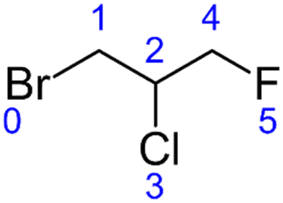
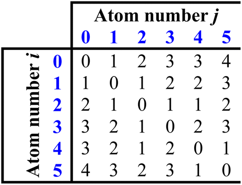
The current version of this SAR is designed to estimate kOH for all acyclic alkanes and haloalkanes of the general formula CnHmX2n+2−m (where X may represent F, Cl, Br or I). The calculation of the E-state of each atom forms the basis of the SAR estimation method. This approach has been described in detail elsewhere16 and has been implemented in the present work without modification. Therefore, we will describe it here only briefly in the context of a worked example:Taking the structure of the halocarbon 1-bromo-2-chloro-3-fluoropropane as a starting point, a hydrogen-suppressed chemical graph is used to represent the molecule, where atom numbers are shown in blue:
From this structure, a distance matrix is constructed, where each element represents the distance, rij, (i.e. the number of chemical bonds) between the ith and jth atom:
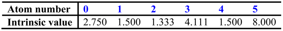
At the same time, the intrinsic values (i.e. a description of the inherent electronic character) of each atom, Ii, can be calculated from the following equation:
| I = (δv + 1)/δ | (1) |
| I = [(2/N)2δv + 1]/δ | (2) |
For an in-depth discussion of this calculation, readers are referred to the original work of Hall et al.16
To begin with, eqn (1) and (2) are employed to produce the following array:
The next step is to generate a matrix that describes the electronic effect that the ith and jth atoms have on each other, with each element defined as (Ii − Ij)/(rij + 1)2:
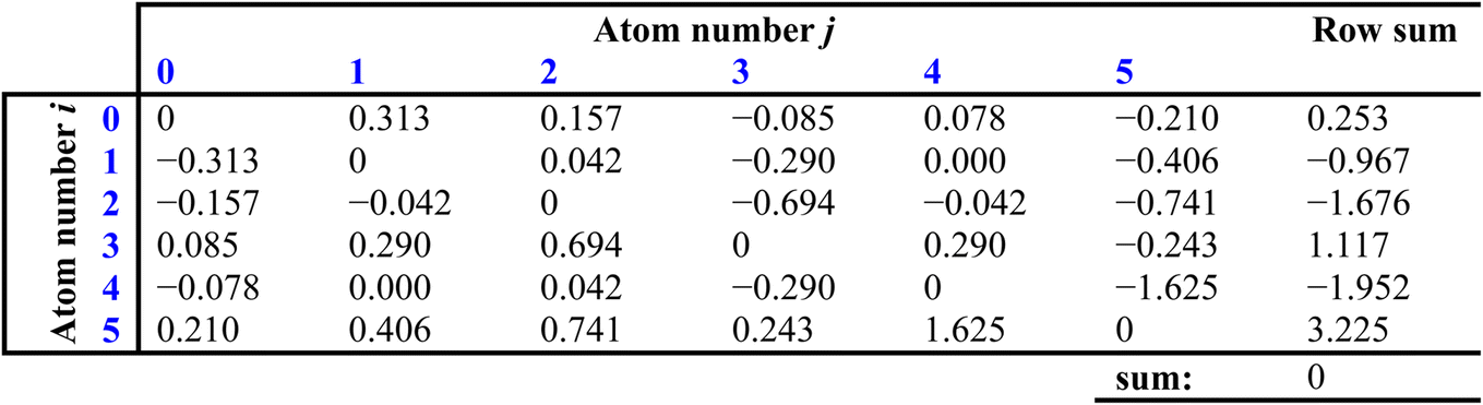
The sums of each row then provide perturbation terms, ΔIi, which describe the overall electronic effect experienced by the ith atom. When ΔIi is added to Ii, this provides the E-state array, Si:
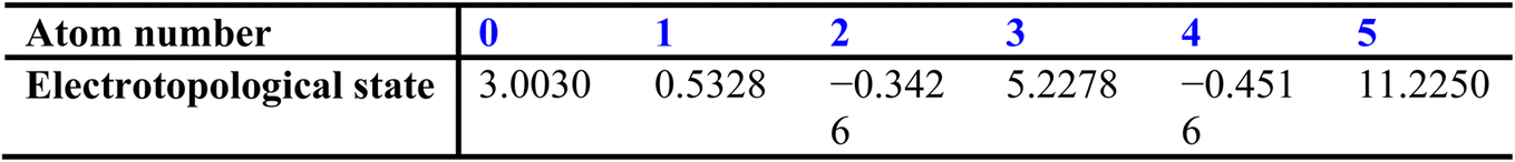
Next, the hydrogen count (nH) attached to each atom is considered:

Reactive C–H bonds were classified by their degree of alkylation (in the case of the CnHmX2n+2−m: primary, secondary or tertiary), and were fitted with a different polynomial expression in each case to yield the site-specific room temperature rate coefficient, ki:
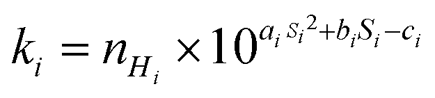 | (3) |
The use of different polynomials based on hydrogen environment was decided empirically, but its necessity can be rationalized from the concept that reaction rate coefficients are defined by enthalpic and entropic terms relating to barrier heights and steric aspects. Given that we don't anticipate a simple relationship between electronic character and these terms, especially the steric effect, we suggest that these fitting parameters compensate for the variation in reactivity that is observed with the degree of alkylation in the OH reaction.
In order to obtain estimates of ki, the values of ai, bi and ci were optimized to minimize the difference between measurements and predictions using a non-linear generalized reduced gradient solver. Values for fitting coefficients a, b and c for the three different types of C–H bond are provided in Table 1. This leads to a total of 9 adjustable parameters (3 × 3 polynomials) that are necessary for rate coefficient estimation using this approach.
| Hydrogen count | a | b | c |
|---|---|---|---|
| 3 (primary) | 0.235348 | 0.448094 | 15.226433 |
| 2 (secondary) | 0.079290 | 0.770329 | 13.470563 |
| 1 (tertiary) | 0.051234 | 0.723300 | 12.452133 |
In our worked example of 1-bromo-2-chloro-3-fluoropropane, this yields calculated site-specific rate coefficients (in units of cm3 per molecule per s) for H-bearing atoms 1, 2 and 4: k1 = 1.83 × 10⁻¹³, k2 = 2.02 × 10⁻¹³ and k4 = 3.15 × 10⁻¹⁴, and a total rate coefficient, ktot, of 4.17 × 10⁻¹³.
Although these calculations are computationally trivial, it is impractical to perform them manually for large numbers of molecules, therefore we provide an open source software programme for batch-calculation, in which the only required input is a list of SMILES strings31 that can be generated in various software packages such as the opensource project Open Babel.32 Our software is written in Python 3, and makes use of some existing libraries and functions in RDKit33 for generating distance matrices, atom types, hydrogen counts and other structural information, together with some additional code that processes this information to calculate the E-state for every atom and ki for every H-bearing carbon atom in the molecule (for Python script, see ESI†). This programme outputs total rate coefficients, together with site-specific rate coefficients and their associated carbon-centred radical products provided in SMILES notation.
2.2. Atkinson group-additivity SAR calculations
The group-additivity approach of Atkinson and co-workers has been documented in detail elsewhere, e.g.9 In short, the Atkinson method considers three group rate coefficients distinguished by their degree of alkylation: kprim, ksec and ktert, and modifies these values according to their substituents using multiplicative F-factors in the following equations:| k(CH3–X) = kprimF(X) | (4) |
| k(X–CH2–Y) = ksecF(X)F(Y) | (5) |
| k[X–CH(–Y)–Z] = ktertF(X)F(Y)F(Z) | (6) |
In this case, we used a version of this algorithm that is provided by the AOPWIN/EPI Suite software package,27 in which we employed the batch-mode of AOPWIN to generate estimates from lists of SMILES strings.
Unlike the E-state method, these F-factors do not possess a physical basis, they are fitting parameters that optimize eqn (4)–(6) to match experimental data. In the current version of AOPWIN, the number of F-factors that pertain to the CnHmX2n+2−m set amounts to 32, which together with the three group rate coefficients totals 35. (See Table S2† for a comprehensive list of these factors). It is noted that some of these F-factors are treated as the same value in this implementation, and so, depending on the interpretation, the adjustable parameter count could be as low as 28.
2.3. DeMore group-additivity SAR calculations
Despite its apparent good performance,34 automated calculations for the group-additivity method of DeMore35 are to our knowledge unavailable, and were performed manually in this case, using the method described in the original paper. As a consequence, our assessments of this SAR's performance were restricted to comparisons with the experimental database, since it was impractical for us to assess the performance of this method in the larger estimation-space.The method of DeMore can be considered to be similar to Atkinson's approach, although it possesses some algorithmic differences. It is based on the following equation:
| logk = logk(CH4) + G1⋯G3 | (7) |
In this case, the G-factors perform an equivalent role to the abovementioned F-factors. One of the key differences of this method is its treatment of sites with more than two substituents, whereby it employs a “3rd-group multiplier”. This serves to limit the electronic effect on heavily substituted reaction sites. The strength of the G-factor is therefore to some extent constrained by the other substitutions on the site, and in this sense, it can be considered to be broadly analogous to the perturbation term (ΔIi) of the E-state method, albeit in a much-simplified form. In total, there are 20 adjustable parameters that are used for making predictions of the CnHmX2n+2−m set, although it is noted that in its current version the coverage of the DeMore method is incomplete. In order to extend it towards iodinated species, and structures with C>1 non-halogenated side-chain lengths, this number would likely approach that of the Atkinson method.
2.4. Ionization potential correlation calculations
The LFER between IP and k298 to predict oxidation rate coefficients has been demonstrated previously for various systems including OH + alkanes36 and OH + hydrofluorocarbons,28 and here, we extend the correlation to all members of the CnHmX2n+2−m set. Although IP as a quantity can be obtained accurately through measurements, these are not available in many cases. Therefore, in order to automatically generate IP estimates, these must be calculated based on chemical structural input. Furthermore, this process must be rapid enough that they can be performed for long lists of molecules within a practical timeframe. For this purpose, the PM6 method29 that is available in MOPAC2016 (ref. 30) was used. To verify the accuracy of the PM6 calculations, they were compared with literature values (where these were available) from the NIST Webbook.37In order to batch calculate IPs, it was necessary to convert SMILES notation into MOPAC2016 input files (.mop). Here, Open Babel32 was used in the command line to generate a sequence of input files, which were subsequently passed to MOPAC2016 (ref. 30) using an appropriate batch file. Once these calculations were performed, output files were parsed using a Python script, to obtain IP values which were then corrected to account for differences between experimental and calculated values.
Ionization potential is a molecular property, rather than one that pertains to any specific reaction site. As such, whereas a rate coefficient will increase additively as the number of abstractable hydrogen atoms increases, its correlate, IP will only be affected by the single-most loosely bound electron within a molecule. This becomes most apparent in members of homologous series with large hydrogen counts, whose rate coefficients are high, yet whose IPs remain largely unchanged compared with the smaller homologues. To account for this, the correlation is first performed on the rate coefficients that have been normalized to the number of hydrogen atoms:
| k/nH = 10(−0.70 × IP + 5.62) | (8) |
2.5. Generation of enumerated lists of the CnHmX2n+2−m set
To generate complete lists of the CnHmX2n+2−m set between carbon numbers 1–4, the MOLGEN 5.04 software package was used.38 These lists can be generated for each carbon number by inputting “fuzzy” molecular formulas into the MOLGEN software in the command line (MS-DOS prompt) using the following commands (interested readers are directed to the MOLGEN 5.04 instruction manual for further information):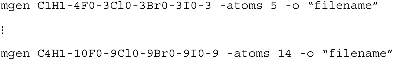
MOLGEN was used to enumerate the CnHmX2n+2−m set up to 8 carbon atoms, and we compare the number of possible isomers with that of experimental determinations in Fig. 1. Because of the rapid growth of this set with carbon number, we restricted our analysis up to a carbon number of 4, which already generates 150665 structures and was considered adequate for our study. Many members of the CnHmX2n+2−m set possess chiral centres and their associated optical isomers. These were not included in the isomer count, since enantiomers will yield identical estimates and are expected to react in an identical way in the hydrogen abstraction reaction.
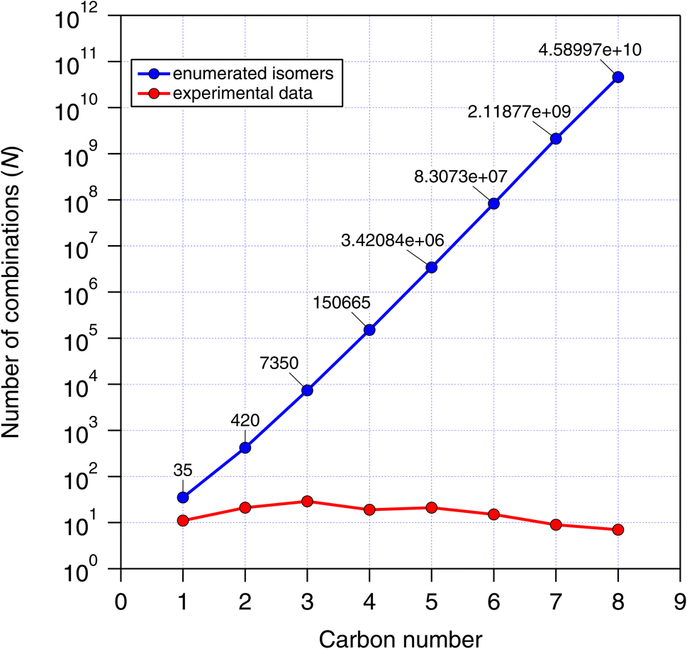 | ||
| Fig. 1 All possible isomers for the CnHmX2n+2−m set (blue) plotted as a function of carbon number. For comparison purposes, the number of isomers with experimental measurements (red) are also presented. | ||
Because this method requires proprietary software that may not be readily available to the readership, as an alternative, this set of compounds can be visualized as a series of Markush structures (see Fig. 2).
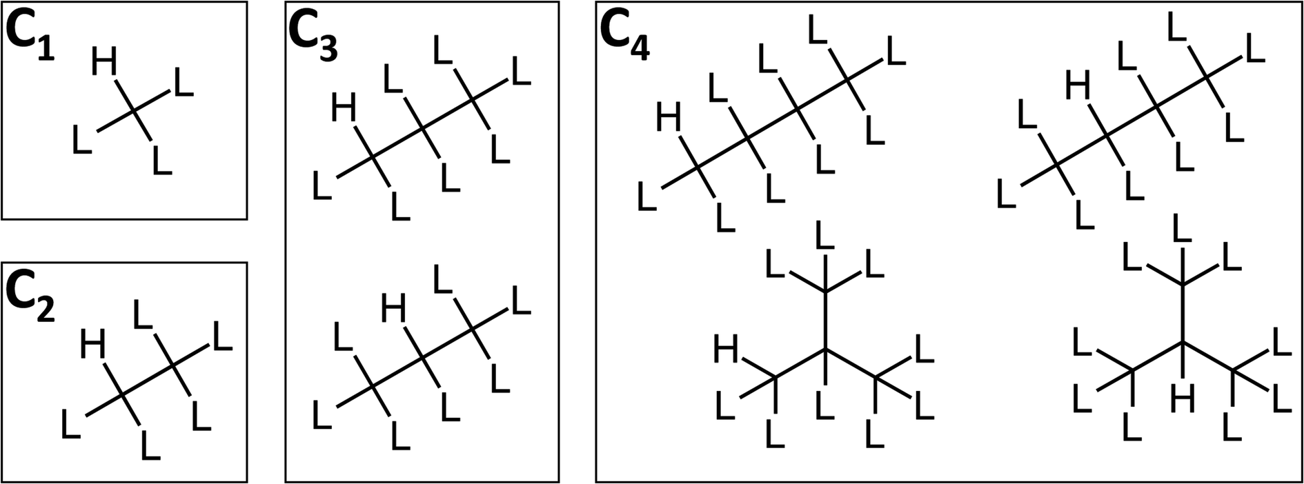 | ||
| Fig. 2 Markush structures for the CnHmX2n+2−m set containing at least one hydrogen atom, where L represents H, F, Cl, Br or I. The position of these hydrogen atoms can vary (in molecules of C≥3), as can the structure of the carbon chain (in molecules of C≥4). As a consequence, the number of Markush structures increases with carbon number according to the well-studied sequence: number of rooted ternary trees with n nodes; number of n-carbon alkyl radicals C(n)H(2n + 1) ignoring stereoisomers.39 | ||
Such structures, if produced in freeware such as MarvinSketch can be rendered as MDL extended molfiles (v3000), which encode sufficient information that can, in principle, be enumerated in much the same way using other software packages. However, we have yet to locate a freely available and convenient approach for doing this at the time of writing.
The structures in the CnHmX2n+2−m set can be subdivided into 7 categories: alkanes (CnH2n+2), fluoroalkanes (CnHmF2n+2−m), chloroalkanes (CnHmCl2n+2−m), bromoalkanes (CnHmBr2n+2−m), iodoalkanes (CnHmI2n+2−m), hydrofluorochlorocarbons (HCFCs) (CnClpFqH2n+2−p−q) and halons (CnXpYqH2n+2−p−q), where n and m are defined as above, p and q ≠ 0, and where X and Y represent any combination of halogens in which at least one possesses a quantum number above that of chlorine. Inspection of these categories shows that at each carbon number, the halons are the most numerous group of compounds (see Fig. 3). The contribution of other groups drops off sharply with increasing carbon number, and by a carbon number of 4, the contribution of all other groups towards the total number of isomers is reduced to a negligible fraction. Therefore, as carbon number increases, the comparisons of estimates in the CnHmX2n+2−m set (see Fig. 3), can be viewed increasingly as a comparison of OH + halon estimates.
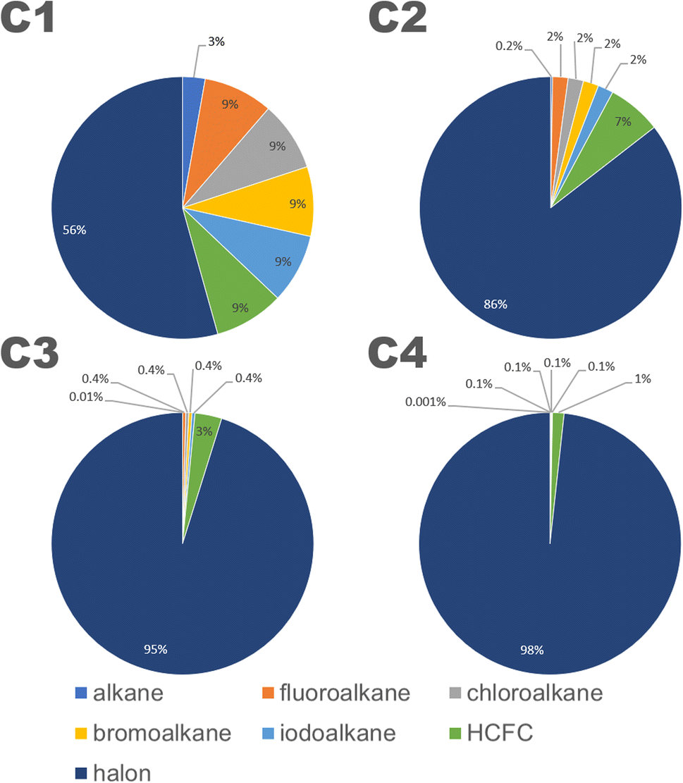 | ||
| Fig. 3 The categories of compounds contained within the CnHmX2n+2−m set separated by carbon number. Halons represent the most numerous fraction at all carbon numbers, and the dominance of this category increases strongly as a function of carbon number. | ||
3. Results and discussion
3.1. Comparisons with experimental data
Because of the greater number of experimental determinations available at room temperature, first we compare the various estimation techniques with k298 as provided by a subset of the reviewed database of McGillen et al.17 (see Table S1†). It should be noted that whereas the E-state and IP approaches have been optimized on a recently compiled dataset,17 the Atkinson and DeMore methods have been optimized on different datasets. The reasons for this are partly practical, in the Atkinson approach, for example, we did not consider it to be within our current scope and time resources to update this approach in its entirety and produce a new implementation beyond that already provided by AOPWIN. Other reasons were more conceptual, for example, to extend DeMore's approach towards a greater variety of species would require us to make some executive decisions on how this technique should be extended. We refrained from doing this, in the spirit of comparing our approach to parameterization with those of other studies.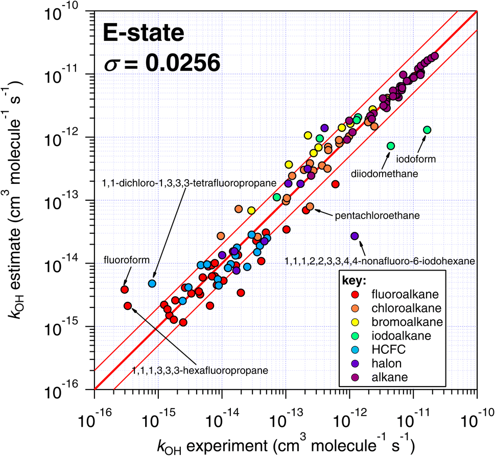 | ||
| Fig. 4 Comparison of k298 estimated using the E-state technique with experimental values. The bold red line represents the 1:1 line, i.e. perfect agreement between observation and estimate, and the lines either side represent a factor of two difference. | ||
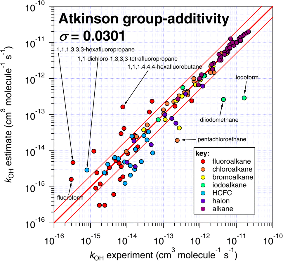 | ||
| Fig. 5 Comparison of k298 estimated using the Atkinson group-additivity technique with experimental values. | ||
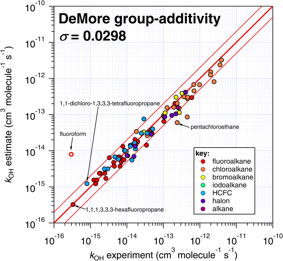 | ||
| Fig. 6 Comparison of k298 estimated using the DeMore group-additivity technique with experimental values. Please note that fluoroform is denoted with an open symbol, which reflects the fact that it was considered to be an exceptional case in the DeMore study.35 We include it here for comparison purposes, since it was included in the other SAR approaches of this study. | ||
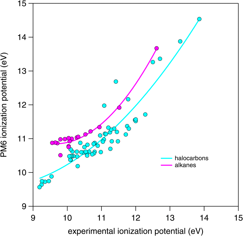 | ||
| Fig. 7 Comparison of PM6 calculated ionization potential with experimental values obtained (where available) from the NIST Standard Reference Database.37 | ||
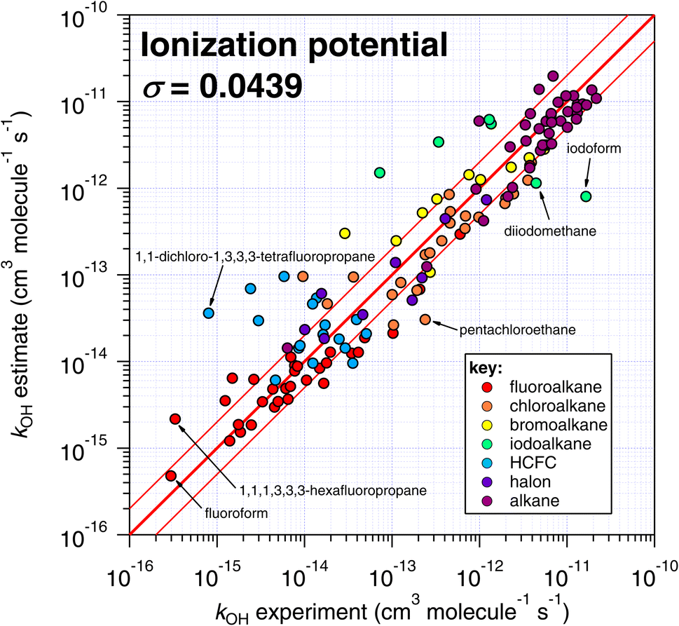 | ||
| Fig. 8 Comparison of k298 estimated using the correlation of IP with experimental values (see Fig. 7). | ||
One interesting outcome from this comparison is the recurrence of outliers between these seemingly disparate techniques. For example, the suspiciously photolabile diiodomethane and iodoform are both significantly underestimated by all applicable techniques: E-state, Atkinson and IP. Pentachloroethane is underestimated by all four techniques. On the other hand, 1,1-dichloro-1,3,3,3-tetrafluoropropane is overestimated by all four methods to a greater or lesser extent. Given that no experimental dataset is perfect, we can hypothesize that some of these errors in the estimation space result from systematic errors in the measurement dataset. There are many more comparisons that can be made in this respect, but an in-depth analysis of this phenomenon is beyond the scope of the current work, which would merit a dedicated publication in order to reach any firm conclusions.
The number of fitting parameters required by each estimation technique is another consideration, since it is possible that in cases where rare or unusual substitution patterns are encountered, overfitting becomes important. In such a scenario, experimental data may be reproduced precisely by poorly constrained fitting factors that compensate for any systematic biases within a given technique. As mentioned above, the purely empirical approaches (Atkinson and DeMore) possess the largest number of fitting factors (28–35 and 20 respectively). By comparison, the more fundamental approaches of E-state and IP require fewer fitting factors (9 and 2 respectively). It is therefore possible that some of the apparently good performance of the Atkinson and DeMore methods can be attributed to the phenomenon of overfitting. Again, a thorough and systematic investigation of this is outside of our intended scope and would warrant a follow-up study. Notwithstanding, the comparatively good performance of the E-state technique with relatively few fitting parameters is a promising outcome, and indicates that it may be relatively reliable outside its immediate training set. The IP method also exhibits a reasonable degree of robustness, with even fewer fitting parameters, albeit with significantly more scatter than the E-state technique.
3.2. Comparisons of site-specificity
Although the total rate coefficient is essential for defining the atmospheric lifetime of a molecule with respect to an oxidation process, for those compounds that contain different reaction sites, site-specific rate coefficients are required in order to assess product distributions. Unfortunately, experimental and quantitative site-specific rate coefficients are very uncommon in the kinetics literature,1 and in this case the only comparisons that we can make are between the site-specific estimates of the SARs themselves (see Fig. 9 and 10).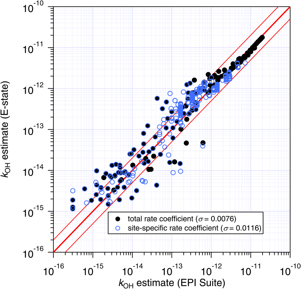 | ||
| Fig. 9 Estimates of k298 and site-specific ki from the E-state technique compared with those of the Atkinson group-additivity approach. In general, better agreement is observed as the total rate coefficient increases, and poorer agreement is observed for site-specific estimates compared with total rate coefficient, which is demonstrated by their respective standard errors (σ) given in parentheses. | ||
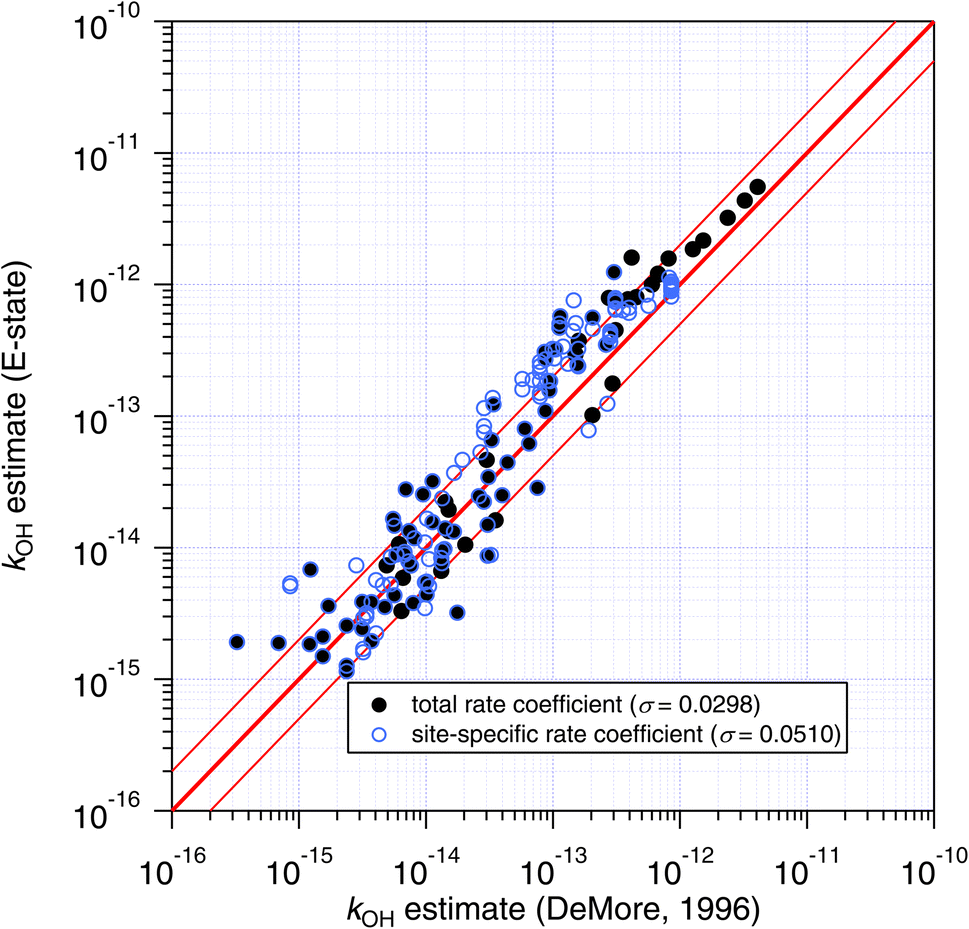 | ||
| Fig. 10 Estimates of k298 and site-specific ki from the E-state technique compared with those of the DeMore group-additivity approach. As with the Atkinson approach, general better agreement is observed for total estimated rate coefficients compared with site-specific ones, as indicated by their respective standard errors (σ) in parentheses. | ||
The site-specific estimates of the Atkinson group-additivity approach were found to be in reasonable agreement with the output from the E-state method, where they follow the same general trend as the total rate coefficient. There is more scatter in the individual estimates which appears to be connected with degeneracy in the site-specific estimates, and is a consequence of the algorithm that is used. For example, in the normal alkanes containing only C and H, the possible number of unique estimates for primary, secondary and tertiary sites is 2, 3 and 4 respectively. In contrast, the E-state technique discriminates between these commonly encountered groups. These different treatments lead to the vertical striping (i.e. degeneracy) in Fig. 9.
The agreement between the E-state and DeMore group-additivity methods is similar to that observed above for the Atkinson approach (see Fig. 10). The main difference is that the numerous and well-predicted larger alkanes are not included in DeMore's approach, which is likely to be responsible for the larger standard errors in the correlation.
Granted the dissimilarity between the algorithms and training sets, the general agreement between all three approaches is encouraging. It appears to confirm (as might be hoped) that even though the F-factors of Atkinson and the G-factors of DeMore are purely fitting factors obtained from linear regressions, that by optimizing their values to a sufficiently large and accurate dataset, these factors contain some fundamental information about the effect of substitution upon reactivity.
3.3. Comparisons of temperature dependence
Many temperature-dependent measurements are available for the reactions of OH + CnHmX2n+2−m, and extend from low (<200 K) to high (>1500 K) temperatures.17 The methodology and performance of the E-state method over this T range is assessed in this section, together with those of Atkinson and DeMore.| Ea/R = m(aiSi2 + biSi − ci) + d | (9) |
With estimates of both k298 and Ea/R, it is possible to estimate the A-factor (A) by rearranging the Arrhenius equation as follows:
 | (10) |
Over a sufficiently large temperature range, abstraction reactions exhibit curvature in their Arrhenius diagrams.17,41 This can be represented in various ways, but for simplicity, we opt for the following extended Arrhenius (i.e. Kooij) equation:
 | (11) |
| n = f + Ea/g | (12) |
Similar to the estimation of room temperature rate coefficients, in order to obtain estimates of k(T), the values of ai, bi, ci, m, d, f and g were optimized to minimize the difference between measurements and predictions using a non-linear generalized reduced gradient solver, the values of which are provided in Table 2. In this instance, estimates and experiments were binned into 23 temperature intervals between 185 and 1507 K. The results of this comparison are shown in Fig. 11, where it is found that estimates tend to agree better with measurements as temperature increases. There are several potential reasons for this, which could be experimental or physico-chemical in nature:
| Polynomial fitting parameters | |||
|---|---|---|---|
| Hydrogen count | a | b | c |
| 3 (primary) | 0.499883684 | 3.4716 × 10⁻⁸ | 15.02936825 |
| 2 (secondary) | 0.071820619 | 0.732006578 | 13.37605256 |
| 1 (tertiary) | 0.044353068 | 0.685568344 | 12.48928548 |
| Temperature-dependent fitting parameters | |||
|---|---|---|---|
| m | d | f | g |
| −199.2590651 | −2242.434844 | 0.797686801 | 2.911224679 |
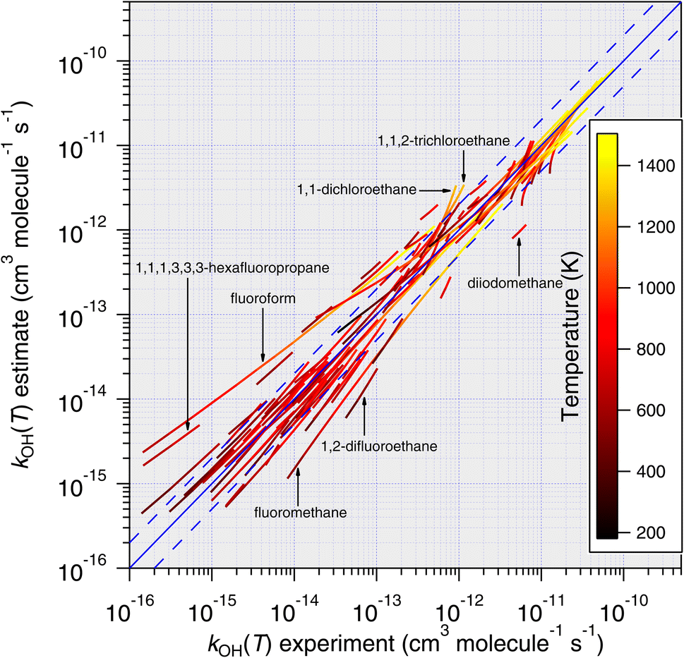 | ||
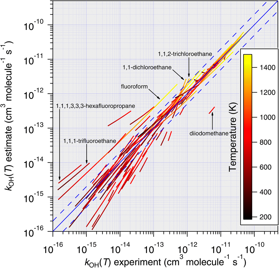
| Fig. 11 Temperature-dependent predictions of k(T) based on the E-state technique, eqn (11), plotted against all available temperature-dependent measurements. With very few exceptions, it is noted that predictions become more accurate as temperature increases. | ||
(1) From the experimental perspective, given that hydrogen abstraction reactions between OH and the CnHmX2n+2−m set exhibit an almost entirely positive temperature dependence, this leads to faster experimental reaction rates at higher temperatures, which tend to be easier to measure. For example, as the rate coefficient becomes smaller, higher reactant concentrations become necessary in the absolute techniques, leading to increasing quenching and decreasing signal to noise ratios in fluorescence-based apparatuses.43 It is also possible that any reactive impurities present35 will possess comparatively low Ea/R, which will become proportionately more important as temperature is decreased. Furthermore, for those compounds that possess lower saturation vapour pressures, a combination of low reactor temperature and high concentration could lead to wall effects that impact the measured rate coefficient at these low temperatures.
(2) For each molecule – and to varying degrees – quantum tunnelling effects on hydrogen abstraction rate coefficients become more significant at lower temperatures.44 This presents an additional condition of the mechanism that the SAR parameterization must satisfy in order to successfully reproduce the experimental observation. The magnitude of the tunnelling transmission coefficients varies by treatment, however, parameterizations of the commonly used Eckart method45 have taken a functional form that may be more complex than our current parameterization can accommodate, e.g.eqn (5), Paraskevas et al. (2015).46
 | ||
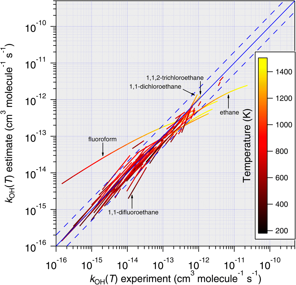
| Fig. 12 Temperature-dependent predictions of k(T) based on the Atkinson group-additivity approach plotted against all available temperature-dependent measurements. More scatter is observed compared with the E-state predictions (see Fig. 11), especially regarding the less reactive molecules in the dataset. However, similar to Fig. 11, predictions are found to improve with increasing temperature. | ||
As with the comparison with the E-state prediction method, better predictions are obtained for more reactive compounds and, in general, predictions become more accurate at higher temperatures. As we mentioned above, there are several potential reasons for this and the same arguments apply in this case. Nevertheless, the overall performance of the group-additivity method is inferior to that of the E-state approach. This is most notable in the underprediction of less reactive compounds in the dataset.
 | ||
| Fig. 13 Temperature-dependent predictions of k(T) based on the DeMore group-additivity approach plotted against all available temperature-dependent measurements. In its current form, this method cannot be applied to all compounds, but applicable compounds are predicted well at lower temperatures. As temperature increases, predictions for some compounds become progressively worse, which is a consequence of the Arrhenius-type parameterization employed. | ||
For the most part, excellent agreement between estimates and experiments is observed, although for compounds whose temperature-dependence has been studied at higher temperatures, the estimates become significantly worse as temperature increases. This is because the unmodified Arrhenius equation forms the basis of this temperature-dependent estimate, which maintains a purely exponential increase in rate coefficient with temperature.
3.4. Comparisons in the larger estimation-space
As noted above, the CnHmX2n+2−m set (see Fig. 1) is far larger than the experimental database, which is comprised of 136 datapoints in the current study. As a result, only a limited subset of values can be tested against experimental determinations. However, a large number of comparisons can be made between different estimation methods, where it is practical to generate estimates in an automated way. Estimates using E-state are compared with the Atkinson group-additivity approach (see Fig. 14) and the IP LFER (see Fig. 15).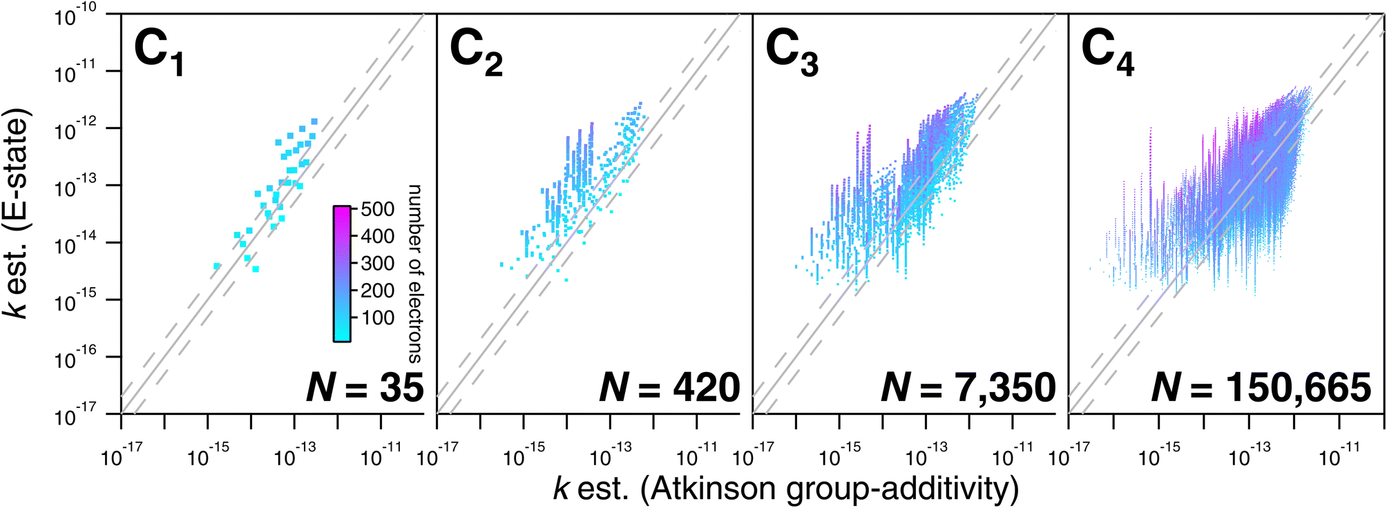 | ||
| Fig. 14 Comparisons of estimated k298 based on the E-state and Atkinson group-additivity approaches for the CnHmX2n+2−m set for values of n ≤ 4. Individual compounds are shaded according to their electron count, from which it can be observed that compounds containing larger numbers of higher quantum number halogens yield systematically lower estimates than the E-state technique. | ||
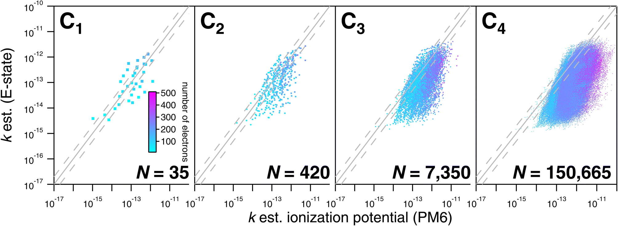 | ||
| Fig. 15 Comparisons of estimated k298 based on the E-state and ionization potential approaches for the CnHmX2n+2−m set for values of n ≤ 4. Better agreement between the ionization potential LFER and the E-state approach is observed for n ≤ 2, beyond which this relationship becomes increasingly diffuse. Larger disagreements between estimates are exhibited by compounds with a larger electron count, where ionization potential estimates are systematically higher. | ||
Regarding comparisons with the Atkinson group-additivity approach, a broad agreement between the techniques is observed, although the degeneracy of the Atkinson algorithm is obvious from C2 and upwards, demonstrated by the prominent vertical stripes in Fig. 14. By colouring species according to their electron count, it becomes apparent that the Atkinson approach produces comparatively high estimates for species with fewer electrons, and lower estimates for those with more. Conversely, for comparisons with the IP technique, no obvious signs of degeneracy are observed in the E-state algorithm or the PM6 calculations (see Fig. 15). However, the agreement between these approaches is generally poorer above C3, becoming somewhat diffuse and appearing to worsen as carbon number is increased. Applying the same colouration as before, it is shown that the largest disagreements are observed in the compounds with higher electron counts.
A graphical representation of the degeneracy of the algorithmic methods of this study is provided in Fig. 16. As expected, the fraction of numerically unique estimates decreases with carbon number (and therefore with the number of isomers). From Fig. 16, it is apparent that this decrease is far more pronounced in the case of the Atkinson group-additivity approach compared with the E-state method.
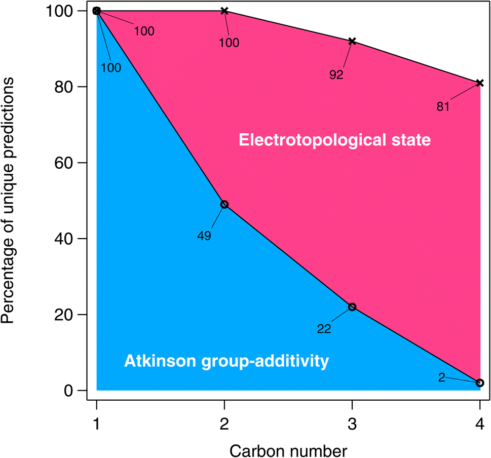 | ||
| Fig. 16 The percentage of unique predictions for the algorithmic methods in the larger estimation-space plotted as a function of carbon number. | ||
Comparisons in the larger estimation space such as those shown in Fig. 14 and 15 are essentially “model-vs-model”, with no direct way of assessing individual estimation accuracy (besides extrapolating their respective performances on the experimental dataset). Nevertheless, we can at least determine some measure of the degree of consensus between techniques within the estimation-space as a whole using descriptive statistics, which provides an indication of the types of molecules for which we can expect the largest degree of uncertainty. For this purpose, standard deviations between estimates were calculated on log-transformed values from the E-state, Atkinson group-additivity and ionization potential approaches for each member of the CnHmX2n+2−m set for n ≤ 4 (see Fig. 17).
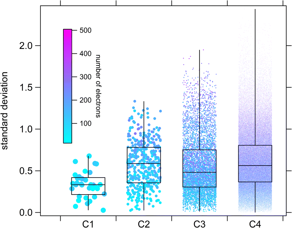 | ||
| Fig. 17 Box-and-whisker diagrams showing the degree of consensus between estimation methods. Here, standard deviations are performed on log-transformed estimates of the OH rate coefficient for each molecule using three techniques: E-state, Atkinson group-additivity and ionization potential correlation. | ||
From Fig. 17 it is observed that medians and interquartile ranges remain largely unchanged between C2 and C4. It is further noted that whereas standard deviation can never drop below zero, the maximum standard deviation is statistically more likely to increase with sample size, which imparts an asymmetrical appearance in the whiskers of this box-and-whisker plot. In order to probe the types of compounds that are likely to produce the largest discrepancies, correlations can be made between standard deviation and some other molecular property. Similar to our treatment in Fig. 14 and 15, we can colour individual estimates according to their electron count, from which we note systematically larger discrepancies in species containing more electrons (i.e. those species with larger numbers of higher quantum number halogen substitutions). There are several potential reasons for this. Firstly, there may be a systematic challenge in calculating IP for these computationally difficult species, even for the diverse parametric method, PM6. Secondly, there are far more kOH measurements for species substituted with F and Cl than there are for Br and I, which may suggest that the training set for the purely empirical Atkinson approach is at present inadequate. Thirdly, although care has been taken to select only high-quality, reviewed kinetic data,17 it is certainly possible, given the difficulties associated with kinetic measurements of photolabile iodinated species, that some of the training data is imperfect. This could potentially lead to increasing divergence in estimation techniques under more extreme conditions (e.g. large numbers of iodine substitutions). Whichever of these interpretations is correct, it is clear that improving the quality and number of experimental observations of this type of compound would be a useful target in order to further improve general SAR performance for the CnHmX2n+2−m set and help to resolve some of these discrepancies.
3.5. The relationship between the electrotopological state and bond-dissociation energy
In Section 3, we have demonstrated the robust and apparently reliable performance of the E-state method towards OH rate coefficient estimation for alkanes and haloalkanes. However, we find it instructive to consider why this simple correlation works in the first place. In this proof-of-principle study, we selected a family of compounds, the CnHmX2n+2−m set, whose OH rate coefficients are expected to decrease as electrons are withdrawn from C–H bonds in these systems. These C–H bonds are shorter and stronger than their more electron-supplied counterparts. We therefore anticipated – given its skill in describing OH rate coefficients – that the E-state, Si, will correlate with bond-dissociation energies (BDEs) of the CnHmX2n+2−m set in accordance with the Evans–Polanyi principle.50 In fact, when Si is correlated with experimental BDEs, BDE(experimental), where n = 1,51 the results were initially underwhelming (see left panel, Fig. 18). However, when this correlation is applied to a purportedly chemically accurate machine-learning approach,52 BDE(ML), and is extended to a fully enumerated set for n = 1, we observe a clustered appearance to this correlation which we found to correspond to the F atom count.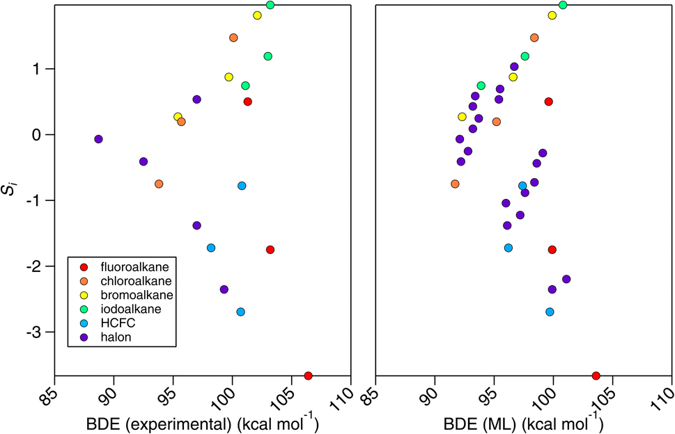 | ||
| Fig. 18 Correlations between the electrotopological state (Si) and the bond-dissociation energy (BDE) for substituted methanes. Left panel: correlation with experimental BDEs.51 Right panel: correlation with BDEs computed from a machine-learning technique.52 Four clusters of points can be observed. This relates to F-atom counts of 0–3 in the CnHmX2n+2−m set where n = 1. | ||
Accordingly, a simple correction to Si was applied in order to yield BDE(E-state):
| BDE(E-state) = (Si + nF × w)m + c | (13) |
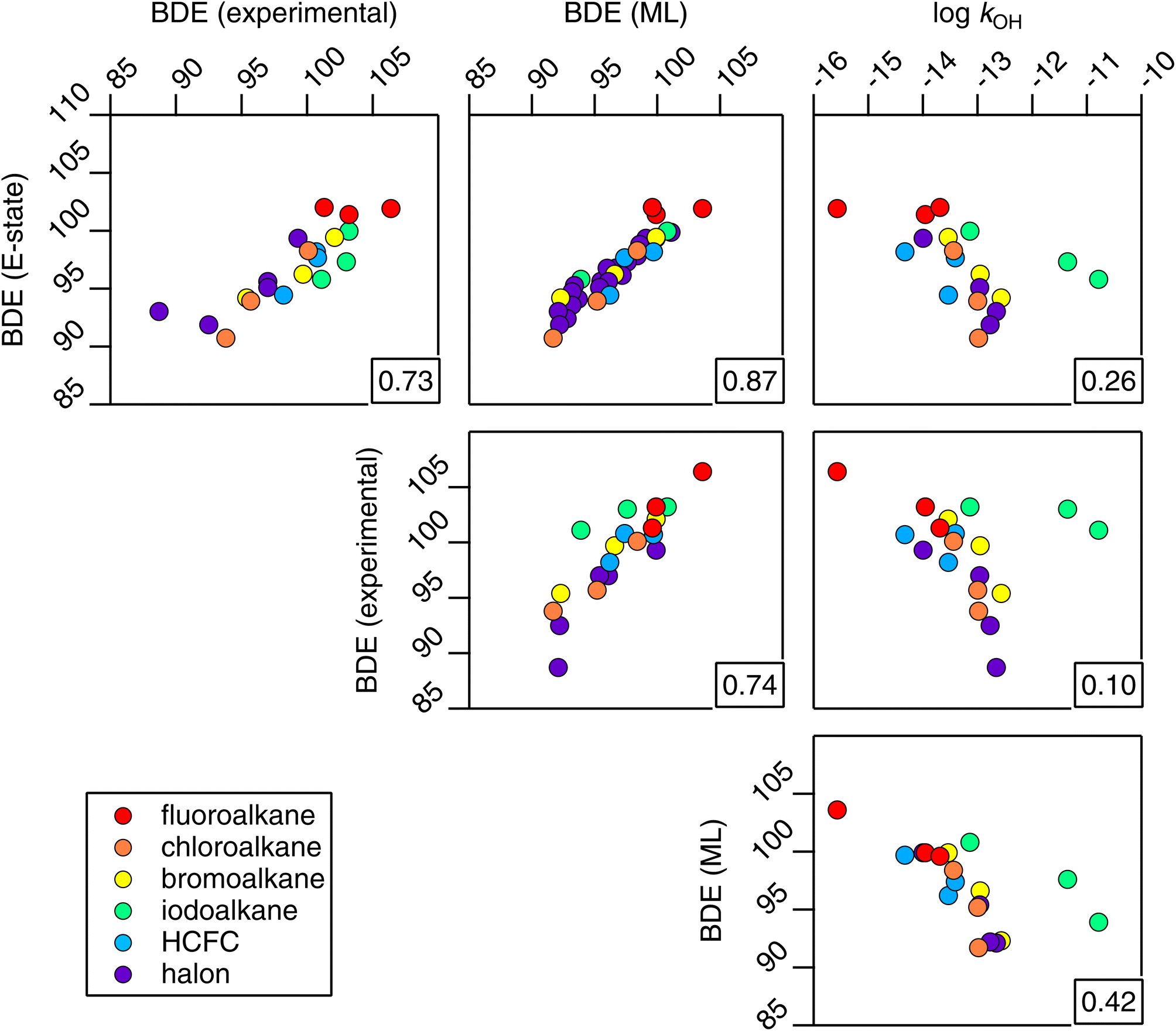 | ||
| Fig. 19 A correlation matrix of bond-dissociation energies estimated from E-state and machine-learning approaches, BDE(E-state) and BDE(ML) respectively, together with experimental BDE and kOH data. The correlation coefficient for each relationship is provided in the bottom right corner of each panel. | ||
One notable finding from the relationship with BDE is that the E-state appears to contain a similar amount of information compared with the far more complicated machine-learning approach,52 which requires an extensive collection of quantum chemical data (R2 = 0.87). In fact, it is not known at the present time which of the two is more accurate, since relationships with experimental data are comparable (R2 = 0.73 and 0.74 respectively), and since the experiments themselves are not without uncertainties. Furthermore, similar to the problems outlined above, for systems containing higher electron counts, it is possible that the performance of a machine-learning technique that depends on quantum chemical data will become less accurate for larger molecules. We anticipate that further work will be necessary in order to make firm conclusions on these points, and also to determine whether BDEs modified for fluorination may provide a viable estimation tool for kOH in hydrogen abstraction reactions.
4. Conclusions
We present a new chemical graph theoretical approach to rate coefficient estimation based on an electrotopological index. Although the potential use of topological indices for oxidation rate coefficient estimation has been explored previously,36,53–56 to the best of our knowledge, this is the first successful application of the electrotopological state towards estimating temperature-dependent, site-specific oxidation rate coefficients. In its application to the CnHmX2n+2−m set, this novel technique is found to represent an improvement over existing SAR algorithms and LFERs, such as the popular Atkinson group-additivity and ionization potential methods.One of the main advantages of SAR approaches is their ability to provide rapid estimates for large lists of compounds. With this in mind, we provide an opensource Python-based programme that enables rapid and automated rate coefficient calculations. We use this software to study the estimation-space of the fully enumerated CnHmX2n+2−m set up to n = 4. From this, we observe the level of consensus between several techniques and the extent of the degeneracy of the SAR approaches.
Perhaps most interestingly, there are some compelling similarities in output from these different techniques, with estimates of site-specificity and temperature dependence showing excellent consistency for the most part. In the latter case, unusual temperature dependences are highlighted for several chemicals that may indicate experimental difficulties, suggesting that new experiments are warranted.
As a family of compounds, the CnHmX2n+2−m set is of great importance to atmospheric chemistry, especially regarding their role in climate warming and ozone depletion, both of which are highly dependent upon hydrogen abstraction reaction rate coefficients. This study is therefore able to provide fresh insights into the reactivity of the many members of this set that have yet to be experimented upon, which may find utility among atmospheric chemical modellers.
Beyond its initial application towards estimating the kinetics of OH abstraction reactions, E-state demonstrates considerable skill in estimating bond-dissociation energies for the CnHmX2n+2−m set, and compares well with experimental data51 and cutting-edge machine-learning methods.52
The electrotopological state represents an information-rich independent variable for describing chemical reactivity. It provides site-specific information on the reactivity of each atom of a molecule and accounts for the electronic interactions of all atoms present in that molecule. This is achieved using an efficient algorithm that requires considerably fewer fitting parameters than existing methods, and with more accuracy than the ionization potential linear free-energy relationship. We have presented its first application to the alkanes and haloalkanes, whose reaction kinetics are simple compared with other volatile species found in the atmosphere. Many of the oxygenated species, for example, will engage in hydrogen-bonded complexation and other mechanistic complications. Notwithstanding, the fundamental nature of the E-state and the level of information that it carries is expected to provide a useful basis for estimating rate coefficients for such species in the future.
Conflicts of interest
There are no conflicts to declare.Acknowledgements
MRM thanks Dr Markus Meringer for some useful discussions on isomer enumeration. MRM, JJO and WPLC thank the Coordinating Research Council (CRC) for their partial support of the project through contract A-108. LM thanks LABEX Voltaire (ANR-10-LABX-100-01).References
- L. Vereecken, B. Aumont, I. Barnes, J. W. Bozzelli, M. J. Goldman, W. H. Green, S. Madronich, M. R. McGillen, A. Mellouki, J. J. Orlando, B. Picquet-Varrault, A. R. Rickard, W. R. Stockwell, T. J. Wallington and W. P. L. Carter, Int. J. Chem. Kinet., 2018, 50, 435–469 CrossRef CAS.
- B. Aumont, S. Szopa and S. Madronich, Atmos. Chem. Phys., 2005, 5, 2497–2517 CrossRef CAS.
- R. Valorso, B. Aumont, M. Camredon, T. Raventos-Duran, C. Mouchel-Vallon, N. L. Ng, J. H. Seinfeld, J. Lee-Taylor and S. Madronich, Atmos. Chem. Phys., 2011, 11, 6895–6910 CrossRef CAS.
- F. Battin-Leclerc, E. Blurock, R. Bounaceur, R. Fournet, P.-A. Glaude, O. Herbinet, B. Sirjean and V. Warth, Chem. Soc. Rev., 2011, 40, 4762–4782 RSC.
- J. Gao, L. B. M. Ellis and L. P. Wackett, Nucleic Acids Res., 2010, 38, D488–D491 CrossRef CAS PubMed.
- R. Atkinson, S. M. Aschmann, W. P. L. Carter, A. M. Winer and J. N. Pitts, Int. J. Chem. Kinet., 1982, 14, 781–788 CrossRef CAS.
- R. Atkinson, Chem. Rev., 1986, 86, 69–201 CrossRef CAS.
- R. Atkinson, Int. J. Chem. Kinet., 1987, 19, 799–828 CrossRef CAS.
- E. Kwok and R. Atkinson, Atmos. Environ., 1995, 29, 1685–1695 CrossRef CAS.
- H. L. Bethel, R. Atkinson and J. Arey, Int. J. Chem. Kinet., 2001, 33, 310–316 CrossRef CAS.
- M. E. Jenkin, R. Valorso, B. Aumont, A. R. Rickard and T. J. Wallington, Atmos. Chem. Phys., 2018, 1–54 Search PubMed.
- W. P. L. Carter, Atmosphere, 2021, 12, 1250 CrossRef CAS.
- S. M. Saunders, M. E. Jenkin, R. G. Derwent and M. J. Pilling, Atmos. Chem. Phys., 2003, 3, 161–180 CrossRef CAS.
- W. P. L. Carter, Documentation of the SAPRC-16 Mechanism Generation System. Draft Interim Report to California Air Resources Board Contract 11-761, 2019 Search PubMed.
- N. R. Greiner, J. Chem. Phys., 1970, 53, 1070–1076 CrossRef CAS.
- L. H. Hall, B. Mohney and L. B. Kier, J. Chem. Inf. Model., 1991, 31, 76–82 CrossRef CAS.
- M. R. McGillen, W. P. L. Carter, A. Mellouki, J. J. Orlando, B. Picquet-Varrault and T. J. Wallington, Earth System Science Data, 2020, 12, 1203–1216 CrossRef.
- WMO, Scientific assessment of ozone depletion: 2018, 2019 Search PubMed.
- H. El Othmani, Y. Ren, Y. Bedjanian, S. El Hajjaji, C. Tovar, P. Wiesen, A. Mellouki, M. R. McGillen and V. Daële, ACS Earth Space Chem., 2021, 5, 960–968 CrossRef CAS.
- H. El Othmani, Y. Ren, A. Mellouki, V. Daële and M. R. McGillen, Chem. Phys. Lett., 2021, 783, 139056 CrossRef CAS.
- M. R. McGillen, M. Baasandorj and J. B. Burkholder, J. Phys. Chem. A, 2013, 117, 4636–4656 CrossRef CAS PubMed.
- D. E. Heard, Acc. Chem. Res., 2018, 51, 2620–2627 CrossRef CAS PubMed.
- I. W. M. Smith and A. R. Ravishankara, J. Phys. Chem. A, 2002, 106, 4798–4807 CrossRef CAS.
- J. P. Senosiain, S. J. Klippenstein and J. A. Miller, J. Phys. Chem. A, 2006, 110, 6960–6970 CrossRef CAS PubMed.
- M. R. McGillen, C. J. Percival, D. E. Shallcross and J. N. Harvey, Phys. Chem. Chem. Phys., 2007, 9, 4349 RSC.
- L. Michelat, A. Mellouki, A. R. Ravishankara, H. El Othmani, V. C. Papadimitriou, V. Daële and M. R. McGillen, ACS Earth Space Chem., 2022, 6, 3101–3114 CrossRef CAS.
- W. M. Meylan and P. H. Howard, Chemosphere, 1993, 26, 2293–2299 CrossRef CAS.
- C. J. Percival, G. Marston and R. P. Wayne, Atmos. Environ., 1995, 29, 305–311 CrossRef CAS.
- J. J. P. Stewart, J. Mol. Model., 2007, 13, 1173–1213 CrossRef CAS PubMed.
- J. J. P. Stewart, MOPAC2016 Stewart Computational Chemistry, Colorado Springs, CO, USA, 2016 Search PubMed.
- D. Weininger, J. Chem. Inf. Comput. Sci., 1988, 28, 31–36 CrossRef CAS.
- N. M. O’Boyle, M. Banck, C. A. James, C. Morley, T. Vandermeersch and G. R. Hutchison, J. Cheminf., 2011, 3, 33 Search PubMed.
- G. Landrum, P. Tosco, B. Kelley, Ric, Sriniker, Gedeck, R. Vianello, D. Cosgrove, N. Schneider, E. Kawashima, D. N., A. Dalke, G. Jones, B. Cole, M. Swain, S. Turk, A. Savelyev, A. Vaucher, M. Wójcikowski, I. Take, D. Probst, K. Ujihara, V. F. Scalfani, G. Godin, A. Pahl, F. Berenger, J. L. Varjo, Strets123, J. P. and D. Gavid, rdkit/rdkit (Version Release_2022_09_3), Zenodo, 2022 Search PubMed.
- D. K. Papanastasiou, A. Beltrone, P. Marshall and J. B. Burkholder, Atmos. Chem. Phys., 2018, 18, 6317–6330 CrossRef CAS.
- W. B. DeMore, J. Phys. Chem., 1996, 100, 5813–5820 CrossRef CAS.
- M. R. McGillen, C. J. Percival, T. Raventos-Duran, G. Sanchez-Reyna and D. E. Shallcross, Atmos. Environ., 2006, 40, 2488–2500 CrossRef CAS.
- P. Linstrom, NIST Chemistry WebBook, NIST Standard Reference Database 69, 1997, DOI:10.18434/T4D303.
- R. Gugisch, A. Kerber, A. Kohnert, R. Laue, M. Meringer, C. Rücker and A. Wassermann, in Advances in Mathematical Chemistry and Applications, Bentham Science Publishers, 2015, vol. 1, pp. 113–138 Search PubMed.
- OEIS Foundation Inc., Number of rooted ternary trees with n nodes; number of n-carbon alkyl radicals C(n)H(2n + 1) ignoring stereoisomers, Entry A000598 in the On-Line Encyclopedia of Integer Sequences, https://oeis.org/A000598.
- W. B. DeMore, J. Photochem. Photobiol., A, 2005, 176, 129–135 CrossRef CAS.
- W. C. Gardiner, Acc. Chem. Res., 1977, 10, 326–331 CrossRef CAS.
- D. R. Burgess and J. A. Manion, J. Phys. Chem. Ref. Data, 2021, 50, 023102 CrossRef CAS.
- M. R. McGillen, F. Bernard, E. L. Fleming and J. B. Burkholder, Geophys. Res. Lett., 2015, 42, 6098–6105 CrossRef CAS.
- A. G. Vandeputte, M. K. Sabbe, M.-F. Reyniers, V. Van Speybroeck, M. Waroquier and G. B. Marin, J. Phys. Chem. A, 2007, 111, 11771–11786 CrossRef CAS PubMed.
- C. Eckart, Phys. Rev., 1930, 35, 1303–1309 CrossRef CAS.
- P. D. Paraskevas, M. K. Sabbe, M.-F. Reyniers, N. G. Papayannakos and G. B. Marin, J. Phys. Chem. A, 2015, 119, 6961–6980 CrossRef CAS.
- M. Rossberg, W. Lendle, G. Pfleiderer, A. Tögel, E.-L. Dreher, E. Langer, H. Rassaerts, P. Kleinschmidt, H. Strack, R. Cook, U. Beck, K.-A. Lipper, T. R. Torkelson, E. Löser, K. K. Beutel and T. Mann, in Ullmann's Encyclopedia of Industrial Chemistry, Wiley-VCH Verlag GmbH & Co. KGaA, Weinheim, Germany, 2006, p. a06_233.pub2 Search PubMed.
- Z. Jiang, P. H. Taylor and B. Dellinger, J. Phys. Chem., 1992, 96, 8964–8966 CrossRef CAS.
- P. H. Taylor, Z. Jiang and B. Dellinger, J. Phys. Chem., 1992, 96, 1293–1296 CrossRef CAS.
- M. G. Evans and M. Polanyi, Trans. Faraday Soc., 1936, 32, 1333 RSC.
- Y.-R. Luo, Handbook of Bond Dissociation Energies in Organic Compounds, CRC Press, 2002 Search PubMed.
- P. C. St. John, Y. Guan, Y. Kim, S. Kim and R. S. Paton, Nat. Commun., 2020, 11, 2328 CrossRef.
- M. R. McGillen, J. Crosier, C. J. Percival, G. Sanchez-Reyna and D. E. Shallcross, Chemosphere, 2006, 65, 2035–2044 CrossRef CAS.
- M. R. McGillen, C. J. Percival, G. Pieterse, L. A. Watson and D. E. Shallcross, Atmos. Chem. Phys., 2007, 7, 3559–3569 CrossRef CAS.
- M. Pompe, M. Veber, M. Randić and A. Balaban, Molecules, 2004, 9, 1160–1176 CrossRef PubMed.
- J. Markelj and M. Pompe, Atmos. Environ., 2016, 131, 418–423 CrossRef CAS.
Footnote |
| † Electronic supplementary information (ESI) available. See DOI: https://doi.org/10.1039/d3ea00147d |
| This journal is © The Royal Society of Chemistry 2024 |