
 Open Access Article
 This Open Access Article is licensed under a
 Creative Commons Attribution 3.0 Unported Licence
Predicting melting temperatures across the periodic table with machine learning atomistic potentials†
Christopher M.
Andolina
 a and
Wissam A.
Saidi
*ab
a and
Wissam A.
Saidi
*ab
aDepartment of Mechanical Engineering and Materials Science, University of Pittsburgh, Pittsburgh, PA 15261, USA
bNational Energy Technology Laboratory, United States Department of Energy, Pittsburgh, PA 15236, USA
First published on 18th June 2024
Abstract
Understanding how materials melt is crucial for their practical applications and development, thereby enabling us to predict their behavior in real-world environmental conditions. Accurate computation of melting temperatures (Tm) has been a long-standing pursuit involving various methods for classical potentials and first-principles calculations. However, finding literature Tm references for many elements using a clearly defined set of calculation parameters is rare. Herein we apply deep neural network atomistic potentials (DNPs), trained on density functional theory (DFT) generated datasets, to describe the melting temperature of 20 single-element materials across the Periodic Table using large-scale molecular dynamics simulations. Our results demonstrate high-fidelity with experimental observations and also with calculated reference melting temperatures, yielding an average deviation of less than 18%. We propose a straightforward elemental-group-specific relationship between Tm and cohesive energy for these calculated references to provide reliable DFT specific reference points, which we believe can be readily applied to many materials. Additionally, we compare DNP predictions for three representative elements at external pressures up to 30 GPa in molecular dynamics simulations, revealing reasonable consistency with experimental and DFT literature references despite the lack of explicit training at these high pressures. This work further extends our flexible approach to developing and modifying DNPs to create unique atomistic potentials tailored to describe atomically complex materials under extreme environmental conditions.
1. Introduction
Accurate predictions of a material's melting provide insight into the behavior of materials under real-world and extreme conditions1–4 and can facilitate the discovery of new materials with desirable properties. The melting temperature (Tm) is a critical material parameter in variety of research fields, such as materials science,5–7 metallurgy,8–10 solid-state physics,11–15 and astro/geophysics.3,4 The determination of Tm can be both experimentally and computationally challenging.16 For materials with large Tm (>2000 K) and/or at high pressures (>10 GPa), experimental data are rare due to experimental limitations. Computational Tm prediction has been demonstrated using various approaches (e.g., hysteresis,17–19 two-phase coexistence,20,21 interface pinning,22,23 and other methods24–28) and has been actively explored for decades.24,25,29–36 The two-phase coexistence (TPC) approach employing large supercells (>10![[thin space (1/6-em)]](https://www.rsc.org/images/entities/char_2009.gif) 000 atoms) is considered the “gold standard” for predicting Tm, as this approach relies on very few assumptions.37 However, accurate computational predictions based on first-principles methods, which are accurate and generally predictive, are prohibitively computationally expensive as ensuing calculations are “large” in two domains: the number of atoms in the simulation cell and the length of simulation time.3,29
000 atoms) is considered the “gold standard” for predicting Tm, as this approach relies on very few assumptions.37 However, accurate computational predictions based on first-principles methods, which are accurate and generally predictive, are prohibitively computationally expensive as ensuing calculations are “large” in two domains: the number of atoms in the simulation cell and the length of simulation time.3,29
Machine learning-based atomistic potentials (MLP),38 such as deep neural network potentials (DNPs),38–41 have emerged as promising tools to accelerate molecular dynamics (MD) simulations. These MLPs can provide accurate predictions of various material properties at a much lower computational cost than first-principles methods while providing high-fidelity simulations akin to first-principles calculations.42–45 Recent methodologies using MLPs, such as moment tensor potentials46 and graph neural networks37 have been demonstrated to improve material properties predictions at elevated temperatures, thus highlighting the community's need for accurate, fast, and flexible approaches to calculating these related figures of merit.
Herein, we describe the training of individual element DNPs for predicting Tm for twenty elements across the Periodic Table using molecular dynamics (MD) simulations at finite pressure. For limited systems where data is available, we compare our results with those obtained using traditional methods, such as MD simulations, DFT calculations, and experimental observations. Although some of these MLP approaches depend on extensive training datasets, in this work, we focus our training protocol on limiting the size of the datasets while we evaluate these DNPs using a MD methodology (TPC simulations) known to have a low bias of Tm predictions when used with classical atomistic potentials.
Our study demonstrates the effectiveness of MLPs in predicting Tm yielding accurate values compared to experiments based on simulations using MD simulations executed containing ∼20000 atoms, despite the datasets being trained with a relatively small supercells (<64 atoms). These findings strongly suggest the general applicability of DNPs for studying material properties of a large variety of elements, paving the way for future investigations into the behavior of complex materials under extreme conditions. This work aims to provide a pathway to generate DNP models capable of accurately modeling the melting behavior of materials. Further, this work highlights the value of DNPs as a powerful tool for discovering, designing, and characterizing materials.47–52
2. Computational methods
2.1 General
The training and validation of the initial DNP training datasets are described in detail elsewhere.51,53 We used the LAMMPS54 code with DeePMD-kit(v2.2.1)41 and DeepPOT-SE55 to train DNPs and predict melting temperatures using a simple two-phase coexistence approach.21 We studied twenty elemental systems in this work; we used a supercell of 14 × 14 × 28 to ensure our prediction of the Tm had negligible finite-size effects and a minimal impact of thermal fluctuations. The initial conventional unit cells for each element's groundstate lattice (bcc, diamond cubic, fcc, hcp, orthorhombic, or rhombohedral) configuration were taken from “The Materials Project” database56 (Table S1†).2.2 Training via adaptive learning
We used an adaptive learning approach to improve the previously reported Tm prediction of the initial DNPs, increasing the total configurations <1000 structures during training (Table S2†). An ensemble approach was used to identify new structures to add to these datasets using three randomly seeded DNPs and a NPT ensemble for one hundred ps with one fs timestep. We initially applied two distinct training loops for this work (Fig. 1). The first loop focused on selecting liquid phase structures at temperatures 1.0, 1.2, and 1.4 of each element's bulk experimental melting temperature (Tm, exp) (Table S1†). Only up to five configurations with the largest deviations within a force tolerance of 0.3–1.5 eV Å−1 were selected for generating MD trajectories with VASP.57–60 We then ran NVT as implemented in VASP described in detail previously53 (VASP INCAR parameters61 are provided in the ESI† on GitHub) on each identified structure at the corresponding temperatures; these structures are then added to the training data to generate a new DNP. For the next iteration, we repeated this process but extended the ensemble to include structures at 0.8 and 0.9 Tm, exp. This iterative process continued until the number of structures that matched the force criteria dwindled to less than 0.5 eV Å−1 for all five temperatures. A final loop was run for all elements, adding solid–liquid interface structures; however, improvement of Tm predictions was only observed for Al, Os, Ti, and Zr.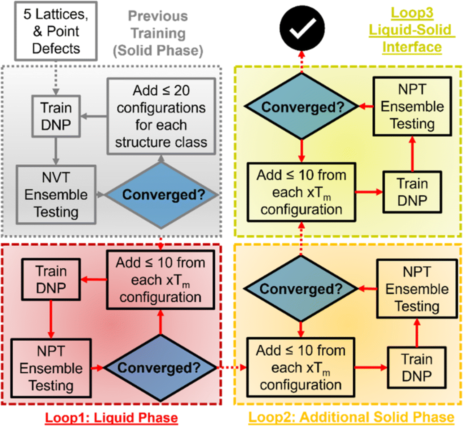 | ||
| Fig. 1 Adaptive learning workflow for developing DNPs for accurate Tm predictions. The first loop adds liquid phase structures at three temperatures (xTm; x = 1, 1.2, and 1.4). The second loop added solid phase structures (xTm; x = 0.8 and 0.9), and the third loop added liquid–solid interface structures (if needed). | ||
2.3 Two-phase coexistence
The DNPs used were first compressed using DeePMD-kit to improve performance for these MD simulations. The simulations were run at finite external pressure, 1.0312 bar (standard atmospheric pressure) or higher for pressure-dependent testing, with an isoenthalpic ensemble (NPH) as implemented in LAMMPS with an equilibration time of one hundred twenty picoseconds (ps) at one femtosecond (fs) timestep to ensure equilibration between the solid and liquid phases. The entire simulation was first heated to melting temperature guess (for convenience, we take Tm, guess = Tm, exp) using NPT with a one hundred fs temperature and one thousand fs pressure damping frequency for ten ps. The lower half of the supercell was assigned as the liquid phase, and the upper half (along the z-axis of the crystal axis) as the solid phase. Next, the liquid phase was heated to approximately 1.25 of the Tm, guess for ten ps, using a NPH ensemble. The statistics for the average Tm of the simulation and standard deviation were calculated from the last twenty ps of the NPH simulation. The impact of the randomly seeded initial velocities was assessed for five distinct simulations for each elemental system with randomly seeded initial velocities. Unless noted otherwise, the errors reported are the same as those of these five simulations. Additionally, we examined the effect of the supercell using 4 × 4 × 8 up to 20 × 20 × 40 supercells for three representative element systems (exploring temperature range, solid phase, and atomic mass) (Li, Ni, and Re). Lastly, using the previously described methods, we explored the accuracy of three selected potentials at higher pressures up to 30 GPa in 5 GPa increments.3. Results and discussion
The TPC MD simulation approach employed to calculate Tm excels in simplicity, i.e., no extraordinary assumptions are made. Using a mixed supercell composed of a solid and liquid phase, Tm is determined when the two phases are in equilibrium, and the melting or crystallization behavior between the phases has stabilized. Our simulations average the total system temperature over many timesteps (20 ps) to predict Tm.29,62 We found that simulations of ∼22000 atoms for these calculations were an acceptable compromise of computation costs and predictive accuracy, vide infra. Starting with our previously developed elemental DNPs,53 we find that these unmodified DNPs predict Tm values with an overall modest accuracy relative to Tm, exp at standard pressure (Fig. S1 and Table S1†) with an average percent error of 24%. We first attempted to rectify the calculated Tm's underestimation of Tm, exp by additional training through an adaptive learning approach. Indeed, we did not expect these original DNPs to describe the melting regime well as they were not trained on the elements' liquid phase, which we had expected would make the TPC calculations challenging.
Therefore, in the first iteration of adaptive learning, we added additional training structures focused on each element's liquid phase (using NPT above the experimental melting temperature at standard pressure) for all elements, see Fig. 1. We gathered results from three randomly seeded DNPs for each element, sampled 100 ps MD trajectories at 1.0, 1.2, and 1.4 multiples of the Tm, exp, and selected configurations for further training that deviated from a set force criterion 0.3 eV Å−1 (Table S2†). No further training was necessary for Li, Mg, or Sr after the first adaptive learning iteration as the largest forces for new structures were <0.05 eV Å−1, well below our threshold. We examined force deviations of liquid, solid, and liquid–solid interfaces for the remaining elements to improve the Tm's prediction. Finally, we re-evaluated basic material benchmark properties (Table S3†), as discussed elsewhere.53 We note improved predictive accuracy compared with DFT for cohesive energy (Ecoh), yielding an average error and standard deviation of <2%.
3.1 Finite-size effects on Tm
Thermal fluctuations in MD simulations increase with increasing temperature and decrease with the number of atoms. Therefore, we use large supercell sizes of +10000 or more atoms to mitigate these inherent noise sources and to improve predictive accuracy. Of course, simulations with so many atoms are highly impractical for DFT calculations due to the high computational costs that would be incurred. Nevertheless, the ease of availability for which atomistic (machine learning) potentials utilize large numbers of atoms and over long timescales (100's of ps), which DFT cannot readily achieve without great computational expense, is a significant asset similar to what has been previously demonstrated for classical potentials (e.g., embedded atom models and modified embedded atom models). This is especially valuable when the atomistic potential training is streamlined and requires less oversight from the operator, a general distinction from previous classical potential developments.
To assess finite-size effects, we investigated three elements with low (Li), moderate (Ni), and high (Nb) experimental melting temperatures (Fig. 1). Due to the stochastic nature of the MD trajectory that depends on how the simulations are initiated, our Tm's are reported as the average obtained from three randomly seeded initial temperature velocities (Table S4†) with the standard error of the mean (sem). Fig. S2† suggests that supercells with ∼22 000 atoms (14 × 14 × 28, fcc conventional unit cell) are sufficiently large to reduce thermal noise to less than 5 K. We find that the employed TCP approach is sensitive to the total number of atoms of the supercell. However, it is challenging to discern if this dependency is solely a result of improving the uncertainty as the number of atoms increases or other finite-size effects, such as long–range interactions. Also, we note, unsurprisingly, that the 1/√N dependence of the sem, with the number of atoms N in the simulation (Fig. 2), is consistent with the fluctuation trends in the canonical ensemble.
 | ||
| Fig. 2 The impact of supercell size N (atoms) on the thermal noise in the simulations of three randomly seeded initial velocity starting points for Li, Ni, and Nb. | ||
To be thorough, we examined the differences in the Tm TPC-DNP results from the final DNP iteration for each element to understand the precision of the randomly seeded DNPs. We find close agreement, as expected, after one or more iterations of adaptive learning training via this stochastic approach. We emphasize the distinction of this analysis from the noise analysis using three randomly seeded initialized velocities (vide supra) compared to this assessment of the DNP training/dataset using three randomly seeding DNPs. For Li, Ni, and Nb, we find that the errors are similar to what we observe from the randomly seeded DNPs (Tables S1, S4, and S5†), suggesting that the potentials are well-trained and that any intrinsic errors are inherent to the accuracies of the DFT approach. These statistical analyses provide not only an assessment of the robustness of the DNP model for MD simulations but also a reasonable estimation of the accuracy of the DNP training and dataset.
Using the simulation protocol of the TPC simulations established and validated for Li, Ni, and Nb, we computed Tm for all selected elements. Fig. 3A (Table S6†) summarizes the DNP as the predicted Tm increases (Re, Mo, Nb, and Os have the largest error), consistent with the expected observations of MD simulations (e.g., increasing thermal noise with increasing temperature). To ensure that finite-size effects in the training data structure for the DNP potential have no appreciable effect, we compared our results with two embedded atom models (EAM) potentials63–65 located in the NIST Interatomic Potential Repository.66 We note that the finite-size impact on Tm is small for these simulation cell ranges (8 × 8 × 16 to 20 × 20 × 40) and is more evident when simulations are under (8 × 8 × 16). Also, results obtained with the MLPs show similar trends in thermal noise reduction as those obtained with the EAM potentials. Furthermore, this comparison suggests that neither the training dataset nor the DNP model shows significant differences from classical potential behaviors (Fig. S3†) regarding finite-size effects.
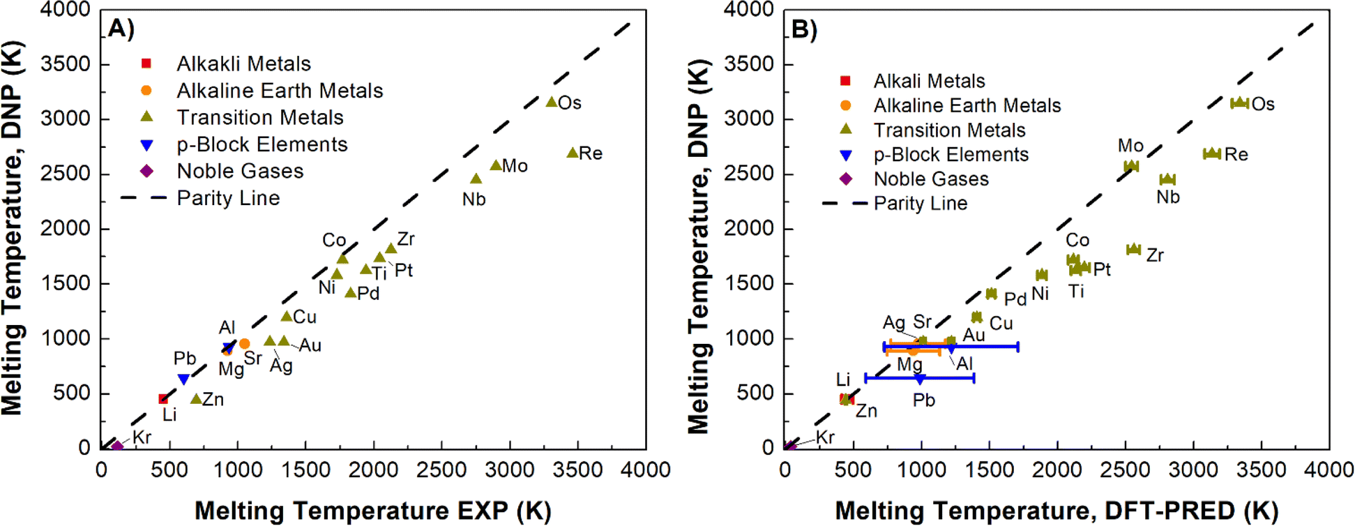 | ||
| Fig. 3 Comparison of the DNP-TPC Tmversus (A) experimental results (R2 = 0.8491) and (B) predicted DFT Tm with (R2 = 0.9896) at standard pressure. Data on the plot are the mean of five MD simulations with randomly seeded initial velocities and the standard error of the mean, some of which are smaller than the plot symbol. In (B), y-errors bar are sems from the five simulations, and the x-errors are associated with the linear fit. The dashed line indicates the parity line. | ||
3.2 DNP-TPC Tm validation
In our initial validation, we elected to compare our findings with experimental reference values over DFT-derived reference values for two reasons: (1) TPC DFT simulations in practice suffer from small supercells and large thermal fluctuations; (2) the DFT reference values in the literature could only be found for ¾ of the investigated elements in this study, namely Ag,67 Al,68 Au,69 Cu,70 Li,71 Mg,72 Mo,73 Ni,74 Os,75 Pb,76 Pd,77 Pt,78 Re,79 Sr,80 and Zr81 (Table S6†). However, we cannot straightforwardly compare these studies given that they are heterogeneous in the adapted computational framework, such as in the exchange-correlation functional, pseudopotentials, DFT codes, and simulation cut-offs. Further, these calculations may be impacted by finite-size effects.There are a handful of recent studies using DNPs to predict Tm. Although the training datasets are more extensive and were developed using different approaches compared to this work, we note relatively good agreement with this literature references for Al (918 ± 5 K),82 Cu (1210 K),83 Mg (870 K),82 and Ti (1886 K)84 with our Tm values of 923 ± 1 K (Al), 1197 ± 1 K (Cu), 911 ± 1 K (Mg), and 1633 ± 13 K (Ti), respectively. Again, there are notable differences between these studies; for example, the authors of the Ti-DNP work did not use TPC but instead a metadynamics approach with smaller supercells than ours for predicting Tm.84 Nevertheless, the overall agreement is compelling and supportive of robust MD modeling using DNP for various phases and elements with good agreement regardless of the dataset composition or specific training approach (e.g., DFT training set generation parameters, and DNP model training parameters, Tm calculation approach, supercell size, etc.). However, noticeable deviations from Tm, exp depend not only on the exchange-correlation functionals27,28,85,86 employed in the DFT calculations but also on other variables such as DFT code, pseudopotentials, energy cut-offs, rather than the MLP model or the adaptive training approach. Therefore, an alternative Tm reference may provide a better understanding of the DNP-TPC accuracy (Fig. 3B), discussed in detail below.
We posit that the DNP underestimation of Tm compared to corresponding experimental values is an artifact propagated from the DFT datasets utilized to train the DNPs (Fig. 3A). Admittedly, it is challenging to show this conclusively, given that accurate and systematic Tm predictions are scarce using DFT with a consistent computational framework, as discussed before. However, as we argue below, this conclusion is strongly suggested, leveraging the empirical correlation between the melting temperature and the system's Ecoh. Overall, underestimating the solid phase binding energies yields a less thermally stable solid phase; therefore, the material's melting point is predicted to occur at lower temperatures than experimentally observed.
Our study used the semi-local Perdew–Burke–Ernzerhof (PBE) functional to generate the DFT training data. Local and semi-local functionals are well-known to have shortcomings due to self-interactions that can only be rectified by accurately including the exact exchange energy, as in hybrid functionals. While PBE reproduces many experimental observables well compared to other semi-local DFT functionals,86 particularly the local-density approximation (LDA), PBE often exhibits lower bond energies.87 This underbinding yields lower Ecoh; see Table S7.† For example, compared to LDA, Zhang et al. noted that PBE provides reasonable Ecoh estimations for main group elements and 3d transition metals (Ti, Co, Cu, and Zn, in this work) but is less accurate for the 4d and 5d transition metals (Zr, Nb, Mo, Pd, Re, Os, Pt, and Au in this work).86 Issues from the exchange–correlation functional could also be a concern for Zn, Ag, Au, and Pt at elevated temperatures and pressures.88
Another factor that influences the melting temperature, which is also compounded by intrinsic inaccuracies of the exchange–correlation functional, is the atomic packing of the lattice. The number of bonds or coordination number (CN) for an atom in orthorhombic, rhombohedral, diamond cubic, bcc, fcc, and hcp lattices are 2, 4, 4, 8, 12, and 12, respectively. The number of bonds in the element's solid phase is larger than the number of bonds in the liquid phase, leading to an underestimation of the propagation of the overall binding energy of the solid phase relative to the liquid phase.37 These coordination numbers are significant in the context of accurate Tm predictions. The bcc (CN = 8) elements evaluated in this work (Li, Ni, and Mo) exhibit remarkable accuracy. We observe increasing average errors (relative to Tm, exp) of 5, 13, and 20% for bcc (3), fcc (9), and hcp (7), respectively. This exemplifies that the transition from solid to liquid for elements with lower CN is generally more accurate than those with more CN (e.g., fcc and hcp).89 Additionally, elements without d-electrons in their outer electron shell required minimal training (Li, Mg, and Sr), and this is consistent with the highly accurate predictions of the initial DNPs without requiring additional training.
3.3 DFT-based prediction of an element's Tm
A well-known empirical relationship exists between an element's Ecoh and the expected Tm value for pure metals (eqn (1)).90 We find a reasonable correlation (R2 = 0.9523) using eqn (1) and DNP-TPC simulations (Fig. S4†). However, we expected better correlations grouping by element.| Tm = 0.032 × Ecoh-EXP/kB | (1) |
Element group-specific linear regression was generated using alkali metals, alkaline earth metals, transition metals, p-block elements, and Noble gases, eqn (2)–(6), respectively. As shown in Fig. 4B, we find that elemental group-specific equations have appreciably better predictions for alkali metals (eqn (2), R2 = 0.9869), alkaline earth metals (eqn (3), R2 = 0.9418), and noble gases (eqn (6), R2 = 0.9992). We also have a simple linear predictive relationship between Tm and Ecoh for all d-block metals (eqn (4), Fig. S5,†R2 = 0.9915). The relationship between Ecoh and Tm of the p-block elements is more complex than that of the other groups discussed. We note that the reactive nonmetal group elements (C, N, O, P, S, and Se), the highly electronegative halogens (F and Cl), and post-transition metals (Ga, In, and Sn) are outliers and were not included in the p-block elements equation (eqn (5), Fig. S6,†R2 = 0.9176). However, this empirical relationship fails to correlate Ecoh and Tm for certain elements, especially the f-block elements, Fig. S7.† We also note a correlation (R2 = 0.9409), Fig. S8† between Ecoh (DFT) and Tm,exp, but these errors are more significant than using the relationships based on experimental Tm and Ecoh.
| Tm = (0.0293 × Ecoh/kB) + 430 K | (2) |
| Tm = (0.0156 × Ecoh/kB) + 162 K | (3) |
| Tm = 0.0346 × Ecoh/kB | (4) |
| Tm = (0.0351 × Ecoh/kB) − 204 K | (5) |
| Tm = (0.0873 × Ecoh/kB) | (6) |
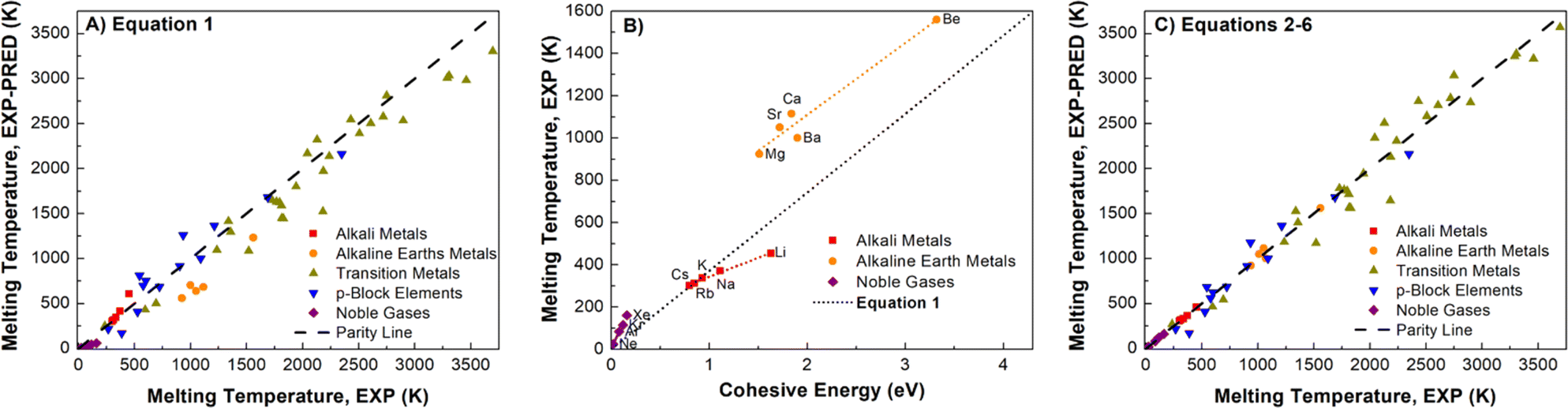 | ||
| Fig. 4 Comparison of non-transition metal elements (A) parity plot showing observed Tm, exp and predicted Tm, exp using eqn (1) (R2 = 0.9857) and (B) Tm, exp and Ecoh and linear fit using eqn (2), (3) and (6), the dotted line represents eqn (1). (C) Tm, exp and Tm, exp predicted using eqn (2)–(6) (R2 = 0.9914). Linear fits in parity plots were forced through the origin. The dashed lines are the parity lines. | ||
Applying eqn (2)–(6) provides accurate predictions of Tm, exp (Fig. 4C). Using experimental Ecoh values, we note that for this data comprised of fifty-five elements, the average % error between the Tm, exp and Tm, exp-pred decreases from 19 to 10%, respectively, for using eqn (1) and (2)–(6) (Table S8†). Extrapolating, we posit that this improvement in correlating cohesive energies and Tm also applies to the DFT values.
We had previously shown excellent agreement with DNP Ecoh values for the corresponding DFT reference values, and this comparison holds even with the additional training data.53
These predictions (using eqn (2)–(6)) are suitable for estimating Tm based on the DFT Ecoh.
3.4 Assessing the robustness of predictions at higher pressures
Lastly, we push the limits of these DNPs further by exploring the Tm predictive accuracy at high pressures (5, 10, 15, 20, 25, and 30 GPa) for select elements (Li, Ni, and Re); see Fig. 5 and Table S10.† We note that we did not explicitly train these potentials at high pressures, only at standard pressure; effectively, we are probing the extent of these DNP's functionality with these compact DFT datasets. However, the distorted lattice structures we used previously to train the initial DNPs53 have some compression, which we anticipate to be likely sufficient to describe these processes at higher pressures. Fig. 5 shows a good agreement of our melting temperature predictions as a function of pressure for these representative systems with literature values. For instance, the non-monotonic Li melting curve profile falls within the bounds of two previous DFT PBE calculations by Tamblyn et al.74 (Fig. 5A). We see an increase in Tm up to 25 GPa and 30 GPa. This anomalous negative slope from ∼10 GPa to 30 GPa is also observed in Na and K, possibly due to the “softening” of phonon modes95,96 and the increasing compressibility of the liquid phase.97–99 The agreement with the experimental results is reasonable;89,92 however, the DFT predictions71,91 are not in agreement, and our DNP results fall between these DFT results, suggesting further research effort is needed to understand why this is observed. One explanation could be that the Li phase change from bcc to fcc at 10–30 GPa accounted for the NVT-based DFT studies, while experimental literature supports this pressure-dependent phase change at this pressure range.100 We observe the fcc phase temperature and pressure regime, which are expected to occur based on experiment.101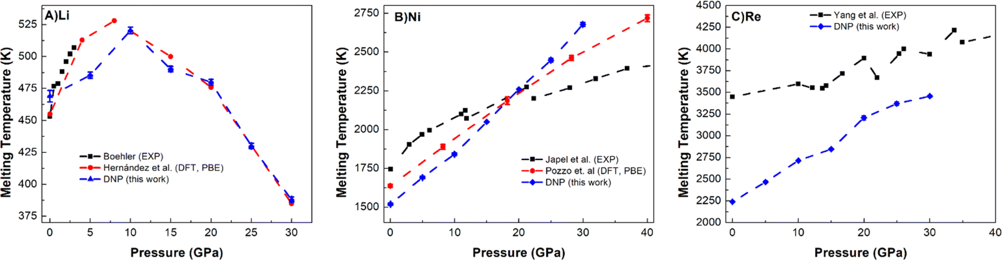 | ||
| Fig. 5 Comparison of DNP TPC Tm values elevated pressures (5, 10, 15, 20, 25, and 30 GPa) with literature values for (A) Li (bcc), (B) Ni (fcc), and (C) Re (hcp). A single MD was run at each DNP point, and the 2σ was smaller than the symbol. DNP-TPC data were compared with reference literature data from first principles 71,74,91 and experiment.89,92–94 The bars shown for Tamblyn et al.91 represent Tm's calculated upper and lower bounds. | ||
The predicted Tm for Ni (Fig. 5B) and Re (Fig. 5C) follow more typical trends in Tm, showing an increase in Tm as pressure increases up to 30 GPa, similar to Ni (ref. 74 and 102) and Re (ref. 93) literature values. Our predictions for Ni agree well with the DFT (PBE) calculations,74 and the agreement is reasonable with experimental observations.89 For Re, we note an agreement with the overall experimental trend for Yang et al. data,93,103 which appears to improve as pressure increases. Interestingly, we could not find any DFT (PBE) calculations in the literature for comparison, and thus, this work may be a first glimpse of what a pressure-dependent Tm curve would show for DFT. These high-temperature and high-pressure calculations and experiments are difficult to conduct,104 exemplified by the few literature reports on Tm and pressure dependence for each method. As the pressure increases, the deviation between DNP/DFT and experiment decreases; this observation has been noted in previous DFT melting simulations for a variety of materials3,30,71,74 and is consistent with lower accuracy of first-principles modeling using PBE functionals at pressures close to zero.88
4. Conclusions
This work highlights the utility of DNPs and the advantages of using large supercells with a two-phase coexistence MD approach to predict the melting temperature of single-element materials with various properties and melting temperatures. We use adaptive learning training to systematically expand these datasets to describe melting temperatures; we demonstrate that the corresponding DNPs generated from compact DFT training sets maintain excellent predictive ability. We show that the accuracy and the thermal noise reduction of the DNP atomistic potentials for Tm prediction are sufficient using a TPC approach when supercells are ∼22 000 (14 × 14 × 28, fcc conventional unit cell). This highly flexible DNP adaptive training approach can be applied to environments outside the DFT training set with high fidelity. The DNPs' prediction of Tm's deviations from the experiment is explained in the context of the intrinsic shortcomings of the PBE functional employed in our study. However, these DNPs allow for predictions with high-fidelity to the first-principles calculations. This approach can be readily adapted to more complex materials and/or evaluated under extreme conditions such as high pressures (e.g., hundreds of GPa) starting from these or the initial DFT-based training set data.Data availability
(1) Data used to generate the main text figures are found in this publication's ESI file.† (2) Due to the large DFT training data file sizes, we have deposited all of the training data to this link (https://www.github.com/saidigroup/20-DNPs-Tm.com). In addition, example validation scripts for both LAMMPs and VASP are archived, as well as the final iterations and all three randomly seeded DNPs for each of the 20 elements discussed in this study.Author contributions
Christopher M. Andolina: conceptualization, data curation, formal analysis, investigation, methodology, resources, software, validation, visualization, writing – original draft. Wissam A. Saidi: conceptualization, formal analysis, funding acquisition, investigation, methodology, project administration, resources, software, supervision, writing – review & editing. Both authors discussed the results and edited the manuscript.Conflicts of interest
There are no conflicts to declare.Acknowledgements
We are grateful to the U.S. National Science Foundation (Award No. CSSI-2003808 and CBET-2130804). Computational support was provided in part by the University of Pittsburgh Center for Research Computing through the resources provided on the H2P cluster, which is supported by NSF (Award No. OAC-2117681).Notes and references
- J. Ma, W. Li, G. Yang, S. Zheng, Y. He, X. Zhang, X. Zhang and X. Zhang, Phys. Earth Planet. Inter., 2020, 309, 106602, DOI:10.1016/j.pepi.2020.106602.
- E. N. Akhmedov, J. Phys. Chem. Solids, 2018, 121, 62–66, DOI:10.1016/j.jpcs.2018.05.011.
- D. Alfe, Phys. Rev. Lett., 2005, 94, 235701, DOI:10.1103/PhysRevLett.94.235701.
- S. Pan, T. Huang, A. Vazan, Z. Liang, C. Liu, J. Wang, C. J. Pickard, H.-T. Wang, D. Xing and J. Sun, Nat. Commun., 2023, 14, 1165 CrossRef CAS PubMed.
- H. Lu, P. Li, Z. Cao and X. Meng, J. Phys. Chem. C, 2009, 113, 7598–7602 CrossRef CAS.
- R. Gregorio and R. Capitao, J. Mater. Sci., 2000, 35, 299–306 CrossRef CAS.
- J. Zhang, B. Song, Q. Wei, D. Bourell and Y. Shi, J. Mater. Sci. Technol., 2019, 35, 270–284 CrossRef CAS.
- T. DebRoy, T. Mukherjee, H. L. Wei, J. W. Elmer and J. O. Milewski, Nat. Rev. Mater., 2021, 6, 48–68, DOI:10.1038/s41578-020-00236-1.
- L. Murr, Addit. Manuf., 2015, 5, 40–53 CAS.
- R. Fandrich, H.-B. Lüngen and C.-D. Wuppermann, Metall. Res. Technol., 2008, 105, 364–374 CAS.
- G. L. Pollack, Rev. Mod. Phys., 1964, 36, 748 CrossRef CAS.
- S. Lou, F. Zhang, C. Fu, M. Chen, Y. Ma, G. Yin and J. Wang, Adv. Mater., 2021, 33, 2000721, DOI:10.1002/adma.202000721.
- L. Qiu, N. Zhu, Y. Feng, E. E. Michaelides, G. Żyła, D. Jing, X. Zhang, P. M. Norris, C. N. Markides and O. Mahian, Phys. Rep., 2020, 843, 1–81 CrossRef CAS.
- B. Lilia, R. Hennig, P. Hirschfeld, G. Profeta, A. Sanna, E. Zurek, W. E. Pickett, M. Amsler, R. Dias and M. I. Eremets, J. Phys.: Condens. Matter, 2022, 34, 183002, DOI:10.1088/1361-648X/ac2864.
- C. Wang, K. Fu, S. P. Kammampata, D. W. McOwen, A. J. Samson, L. Zhang, G. T. Hitz, A. M. Nolan, E. D. Wachsman and Y. Mo, Chem. Rev., 2020, 120, 4257–4300, DOI:10.1021/acs.chemrev.9b00427.
- G. de With, Chem. Rev., 2023, 123, 13713–13795, DOI:10.1021/acs.chemrev.3c00489.
- L. Zheng, Q. An, Y. Xie, Z. Sun and S.-N. Luo, J. Chem. Phys., 2007, 127, 164503, DOI:10.1063/1.2790424.
- S. N. Luo, A. Strachan and D. C. Swift, J. Chem. Phys., 2004, 120 24, 11640–11649, DOI:10.1063/1.1755655.
- Y. W. Tang, J. Wang and X. C. Zeng, J. Chem. Phys., 2006, 124, 236103, DOI:10.1063/1.2206592.
- S. V. Starikov and V. V. Stegailov, Phys. Rev. B: Condens. Matter Mater. Phys., 2009, 80, 220104, DOI:10.1103/PhysRevB.80.220104.
- J. R. Morris, C. Z. Wang, K. M. Ho and C. T. Chan, Phys. Rev. B: Condens. Matter Mater. Phys., 1994, 49, 3109–3115, DOI:10.1103/PhysRevB.49.3109.
- U. R. Pedersen, F. Hummel, G. Kresse, G. Kahl and C. Dellago, Phys. Rev. B: Condens. Matter Mater. Phys., 2013, 88, 094101, DOI:10.1103/PhysRevB.88.094101.
- U. R. Pedersen, J. Chem. Phys., 2013, 139, 104102, DOI:10.1063/1.4818747.
- D. Frenkel and A. J. Ladd, J. Chem. Phys., 1984, 81, 3188–3193 CrossRef CAS.
- G. Grochola, J. Chem. Phys., 2004, 120, 2122–2126 CrossRef CAS PubMed.
- S. Alavi and D. L. Thompson, J. Chem. Phys., 2005, 122, 154704, DOI:10.1063/1.1880932.
- L.-F. Zhu, B. Grabowski and J. Neugebauer, Phys. Rev. B, 2017, 96, 224202, DOI:10.1103/PhysRevB.96.224202.
- L.-F. Zhu, F. Körmann, A. V. Ruban, J. Neugebauer and B. Grabowski, Phys. Rev. B, 2020, 101, 144108, DOI:10.1103/PhysRevB.101.144108.
- Y. Zou, S. Xiang and C. Dai, Comput. Mater. Sci., 2020, 171, 109156, DOI:10.1016/j.commatsci.2019.109156.
- D. Alfe, M. Alfredsson, J. Brodholt, M. Gillan, M. Towler and R. Needs, Phys. Rev. B: Condens. Matter Mater. Phys., 2005, 72, 014114 CrossRef.
- Q.-J. Hong and A. Van De Walle, Phys. Rev. B: Condens. Matter Mater. Phys., 2015, 92, 020104 CrossRef.
- F. Dorner, Z. Sukurma, C. Dellago and G. Kresse, Phys. Rev. Lett., 2018, 121, 195701, DOI:10.1103/PhysRevLett.121.195701.
- L. Chen and V. S. Bryantsev, Phys. Chem. Chem. Phys., 2017, 19, 4114–4124, 10.1039/c6cp08403f.
- G. García, M. Atilhan and S. Aparicio, Chem. Phys. Lett., 2015, 634, 151–155 CrossRef.
- L.-F. Zhu, J. Janssen, S. Ishibashi, F. Körmann, B. Grabowski and J. Neugebauer, Comput. Mater. Sci., 2021, 187, 110065, DOI:10.1016/j.commatsci.2020.110065.
- D. E. Farache, J. C. Verduzco, Z. D. McClure, S. Desai and A. Strachan, Comput. Mater. Sci., 2022, 209, 111386, DOI:10.1016/j.commatsci.2022.111386.
- Q.-J. Hong, Comput. Mater. Sci., 2022, 214, 111684, DOI:10.1016/j.commatsci.2022.111684.
- Y. Zuo, C. Chen, X. Li, Z. Deng, Y. Chen, J. Behler, G. Csányi, A. V. Shapeev, A. P. Thompson, M. A. Wood and S. P. Ong, J. Phys. Chem. A, 2020, 124, 731–745, DOI:10.1021/acs.jpca.9b08723.
- K. Choudhary, B. DeCost, C. Chen, A. Jain, F. Tavazza, R. Cohn, C. W. Park, A. Choudhary, A. Agrawal and S. J. Billinge, npj Comput. Mater., 2022, 8, 59 CrossRef.
- E. Kocer, T. W. Ko and J. Behler, Annu. Rev. Phys. Chem., 2022, 73, 163–186, DOI:10.1146/annurev-physchem-082720-034254.
- H. Wang, L. Zhang, J. Han and E. Weinan, Comput. Phys. Commun., 2018, 228, 178–184 CrossRef CAS.
- C. Cheng, Y. Yang, Y. Zhong, Y. Chen, T. Hsu and J. Yeh, Curr. Opin. Solid State Mater. Sci., 2017, 21, 299 CrossRef CAS.
- M. Haghighatlari, J. Li, X. Guan, O. Zhang, A. Das, C. J. Stein, F. Heidar-Zadeh, M. Liu, M. Head-Gordon and L. Bertels, Digital Discovery, 2022, 1, 333–343, 10.1039/d2dd00008c.
- J. T. Margraf, Angew. Chem., Int. Ed., 2023, 62, e202219170, DOI:10.1002/anie.202219170.
- S. Axelrod, D. Schwalbe-Koda, S. Mohapatra, J. Damewood, K. P. Greenman and R. Gómez-Bombarelli, Acc. Mater. Res., 2022, 3, 343–357 CrossRef CAS.
- J. H. Jung, P. Srinivasan, A. Forslund and B. Grabowski, npj Comput. Mater., 2023, 9, 3, DOI:10.1038/s41524-022-00956-8.
- C. M. Andolina, M. Bon, D. Passerone and W. A. Saidi, J. Phys. Chem. C, 2021, 125, 17438–17447, DOI:10.1021/acs.jpcc.1c04403.
- C. M. Andolina, P. Williamson and W. A. Saidi, J. Chem. Phys., 2020, 152, 154701, DOI:10.1063/5.0005347.
- C. M. Andolina, J. G. Wright, N. Das and W. A. Saidi, Phys. Rev. Mater., 2021, 5, 083804, DOI:10.1103/PhysRevMaterials.5.083804.
- D. Bayerl, C. M. Andolina, S. Dwaraknath and W. A. Saidi, Digital Discovery, 2022, 1, 61–69, 10.1039/d1dd00005e.
- P. Wisesa, C. M. Andolina and W. A. Saidi, Chem. Phys. Lett., 2023, 14, 468–475, DOI:10.1021/acs.jpclett.2c03445.
- W. A. Saidi, npj Comput. Mater., 2022, 8, 86 CrossRef CAS.
- C. M. Andolina and W. A. Saidi, Digital Discovery, 2023, 2, 1070–1077, 10.1039/D3DD00046J.
- S. Plimpton, J. Comput. Phys., 1995, 117, 1–19, DOI:10.1006/jcph.1995.1039.
- L. Zhang, J. Han, H. Wang, W. A. Saidi, R. Car and E. Weinan, 2018.
- A. Jain, S. P. Ong, G. Hautier, W. Chen, W. D. Richards, S. Dacek, S. Cholia, D. Gunter, D. Skinner, G. Ceder and K. A. Persson, APL Mater., 2013, 1, DOI:10.1063/1.4812323.
- G. Kresse and J. Hafner, Phys. Rev. B: Condens. Matter Mater. Phys., 1993, 47, 558–561 CrossRef CAS PubMed.
- G. Kresse and D. Joubert, Phys. Rev. B: Condens. Matter Mater. Phys., 1999, 59, 1758–1775, DOI:10.1103/PhysRevB.59.1758.
- G. Kresse and J. Furthmuller, Phys. Rev. B: Condens. Matter Mater. Phys., 1996, 54, 11169–11186, DOI:10.1103/physrevb.54.11169.
- G. Kresse and J. Furthmuller, Comput. Mater. Sci., 1996, 6, 15–50, DOI:10.1016/0927-0256(96)00008-0.
- General INCAR parameters for each VASP calculation: ENCUT=400 eV, KSPACING=0.24, EDIFF=1e-8, ISMEAR=1, SIGMA=0.15, only the NVT temperature was varied.
- K. Dang, J. Chen, B. Rodgers and S. Fensin, Comput. Phys. Commun., 2023, 286, 108667 CrossRef CAS.
- X.-Y. Liu, P. P. Ohotnicky, J. B. Adams, C. L. Rohrer and R. W. Hyland, Surf. Sci., 1997, 373, 357–370, DOI:10.1016/S0039-6028(96)01154-5.
- M. I. Mendelev, D. J. Srolovitz, G. J. Ackland and S. Han, J. Mater. Res., 2005, 20, 208–218, DOI:10.1557/JMR.2005.0024.
- M. I. Mendelev, M. J. Kramer, C. A. Becker and M. Asta, Philos. Mag., 2008, 88, 1723–1750, DOI:10.1080/14786430802206482.
- NIST Interatomic Potentials Repository, https://www.ctcms.nist.gov/potentials, accessed 05/20/2024, 2024 Search PubMed.
- S. Baty, L. Burakovsky and D. Errandonea, J. Phys.: Condens. Matter, 2021, 33, 485901 CrossRef CAS PubMed.
- J. Bouchet, F. Bottin, G. Jomard and G. Zérah, Phys. Rev. B: Condens. Matter Mater. Phys., 2009, 80, 094102, DOI:10.1103/PhysRevB.80.094102.
- G. Weck, V. Recoules, J.-A. Queyroux, F. Datchi, J. Bouchet, S. Ninet, G. Garbarino, M. Mezouar and P. Loubeyre, Phys. Rev. B, 2020, 101, 014106, DOI:10.1103/PhysRevB.101.014106.
- L. Vočadlo, D. Alfè, G. D. Price and M. J. Gillan, J. Chem. Phys., 2004, 120, 2872–2878, DOI:10.1063/1.1640344.
- E. R. Hernández, A. Rodriguez-Prieto, A. Bergara and D. Alfè, Phys. Rev. Lett., 2010, 104, 185701, DOI:10.1103/PhysRevLett.104.185701.
- C. Cui, J. Xian, H. Liu, F. Tian, X. Gao and H. Song, J. Appl. Phys., 2022, 131, 195901, DOI:10.1063/5.0087764.
- C. Cazorla, M. Gillan, S. Taioli and D. Alfè, J. Chem. Phys., 2007, 126, 194502, DOI:10.1063/1.2735324.
- M. Pozzo and D. Alfè, Phys. Rev. B: Condens. Matter Mater. Phys., 2013, 88, 024111, DOI:10.1103/PhysRevB.88.024111.
- L. Burakovsky, N. Burakovsky and D. Preston, Phys. Rev. B: Condens. Matter Mater. Phys., 2015, 92, 174105 CrossRef.
- T. Bryk, T. Demchuk and N. Jakse, Phys. Rev. B, 2019, 99, 014201, DOI:10.1103/PhysRevB.99.014201.
- Z.-L. Liu, J.-H. Yang, L.-C. Cai, F.-Q. Jing and D. Alfè, Phys. Rev. B: Condens. Matter Mater. Phys., 2011, 83, 144113, DOI:10.1103/PhysRevB.83.144113.
- L. Burakovsky, S. P. Chen, D. L. Preston and D. G. Sheppard, J. Phys.: Conf. Ser., 2014, 500, 162001, DOI:10.1088/1742-6596/500/16/162001.
- D. Minakov, P. Levashov and M. Paramonov, 2019.
- N. Bhatt, P. Vyas and A. Jani, Philos. Mag., 2010, 90, 1599–1622 CrossRef CAS.
- D. Minakov, M. Paramonov, G. Demyanov, V. Fokin and P. Levashov, Phys. Rev. B, 2022, 106, 214105 CrossRef CAS.
- L. Zhang, D.-Y. Lin, H. Wang, R. Car and W. E, Phys. Rev. Mater., 2019, 3, 023804, DOI:10.1103/PhysRevMaterials.3.023804.
- Y. Du, Z. Meng, Q. Yan, C. Wang, Y. Tian, W. Duan, S. Zhang and P. Lin, Phys. Chem. Chem. Phys., 2022, 24, 18361–18369 RSC.
- T. Wen, R. Wang, L. Zhu, L. Zhang, H. Wang, D. J. Srolovitz and Z. Wu, npj Comput. Mater., 2021, 7, 206, DOI:10.1038/s41524-021-00661-y.
- L. Schimka, R. Gaudoin, J. Klimeš, M. Marsman and G. Kresse, Phys. Rev. B: Condens. Matter Mater. Phys., 2013, 87, 214102, DOI:10.1103/PhysRevB.87.214102.
- G. Zhang, New J. Phys., 2018, 20, 063020 CrossRef.
- J. P. Perdew, A. Ruzsinszky, G. I. Csonka, O. A. Vydrov, G. E. Scuseria, L. A. Constantin, X. Zhou and K. Burke, Phys. Rev. Lett., 2008, 100, 136406, DOI:10.1103/PhysRevLett.100.136406.
- A. Dewaele, M. Torrent, P. Loubeyre and M. Mezouar, Phys. Rev. B: Condens. Matter Mater. Phys., 2008, 78, 104102, DOI:10.1103/PhysRevB.78.104102.
- S. Japel, B. Schwager, R. Boehler and M. Ross, Phys. Rev. Lett., 2005, 95, 167801, DOI:10.1103/PhysRevLett.95.167801.
- F. Guinea, J. H. Rose, J. R. Smith and J. Ferrante, Appl. Phys. Lett., 1984, 44, 53–55, DOI:10.1063/1.94549.
- I. Tamblyn, J.-Y. Raty and S. A. Bonev, Phys. Rev. Lett., 2008, 101, 075703, DOI:10.1103/PhysRevLett.101.075703.
- R. Boehler, Phys. Rev. B: Condens. Matter Mater. Phys., 1983, 27, 6754 CrossRef CAS.
- L. Yang, A. Karandikar and R. Boehler, Rev. Sci. Instrum., 2012, 83, 063905, DOI:10.1063/1.4730595.
- A. M. J. Schaeffer, W. B. Talmadge, S. R. Temple and S. Deemyad, Phys. Rev. Lett., 2012, 109, 185702, DOI:10.1103/PhysRevLett.109.185702.
- J.-Y. Raty, E. Schwegler and S. A. Bonev, Nature, 2007, 449, 448–451, DOI:10.1038/nature06123.
- E. R. Hernández and J. Íñiguez, Phys. Rev. Lett., 2007, 98, 055501, DOI:10.1103/PhysRevLett.98.055501.
- M. Martinez-Canales and A. Bergara, J. Phys. Chem. Solids, 2008, 69, 2151–2154, DOI:10.1016/j.jpcs.2008.03.022.
- L. Koči, R. Ahuja, L. Vitos and U. Pinsook, Phys. Rev. B: Condens. Matter Mater. Phys., 2008, 77, 132101, DOI:10.1103/PhysRevB.77.132101.
- S. V. Lepeshkin, M. V. Magnitskaya and E. G. Maksimov, JETP Lett., 2009, 89, 586–591, DOI:10.1134/S0021364009110137.
- A. Lazicki, Y. Fei and R. J. Hemley, Solid State Commun., 2010, 150, 625–627, DOI:10.1016/j.ssc.2009.12.029.
- C. L. Guillaume, E. Gregoryanz, O. Degtyareva, M. I. McMahon, M. Hanfland, S. Evans, M. Guthrie, S. V. Sinogeikin and H. K. Mao, Nat. Phys., 2011, 7, 211–214, DOI:10.1038/nphys1864.
- D. Errandonea, Phys. Rev. B: Condens. Matter Mater. Phys., 2013, 87, 054108 CrossRef.
- L. Burakovsky, N. Burakovsky, D. Preston and S. Simak, Crystals, 2018, 8, 243 CrossRef.
- P. Wisesa, C. M. Andolina and W. A. Saidi, Chem. Phys. Lett., 2023, 14, 8741–8748, DOI:10.1021/acs.jpclett.3c02424.
Footnote |
| † Electronic supplementary information (ESI) available: Details for all DNP and DFT values for each element in the plots. As well as configuration counts and tables of reference experimental, DFT and DNP comparisons. DFT training data, DNPs, and example validation scripts. See DOI: https://doi.org/10.1039/d4dd00069b |
| This journal is © The Royal Society of Chemistry 2024 |