Tailoring phosphine ligands for improved C–H activation: insights from Δ-machine learning

Abstract

Transition metal complexes have played crucial roles in various homogeneous catalytic processes due to their exceptional versatility. This adaptability stems not only from the central metal ions but also from the vast array of choices of the ligand spheres, which form an enormously large chemical space. For example, Rh complexes, with a well-designed ligand sphere, are known to be efficient in catalyzing the C–H activation process in alkanes. To investigate the structure–property relation of the Rh complex and identify the optimal ligand that minimizes the calculated reaction energy ΔE of an alkane C–H activation, we have applied a Δ-machine learning method trained on various features to study 1743 pairs of reactants (Rh(PLP)(Cl)(CO)) and intermediates (Rh(PLP)(Cl)(CO)(H)(propyl)). Our findings demonstrate that the models exhibit robust predictive performance when trained on features derived from electron density (R² = 0.816), and SOAPs (R² = 0.819), a set of position-based descriptors. Leveraging the model trained on xTB-SOAPs that only depend on the xTB-equilibrium structures, we propose an efficient and accurate screening procedure to explore the extensive chemical space of bisphosphine ligands. By applying this screening procedure, we identify ten newly selected reactant–intermediate pairs with an average ΔE of 33.2 kJ mol⁻¹, remarkably lower than the average ΔE of the original data set of 68.0 kJ mol⁻¹. This underscores the efficacy of our screening procedure in pinpointing structures with significantly lower energy levels.

---

1. Introduction

Organometallic compounds have been extensively applied in homogeneous catalytic processes, owing to their versatile redox properties that can be easily tuned and optimized to the specific chemical process of interest. This tunability is achieved through the alteration of the metal center, and more importantly, through structural modification of the ligand sphere. For example, by precisely designing the ligand architecture, Ir- and Rh-based complexes can be applied for the hydrogenation of CO₂ (ref. 1) and olefins,² the oxidation of water,³ the activation of hydrocarbon halides,^4,5 the dehydrogenation of alkanes,^6,7 as well as the carbonylation of alkanes and benzene.^6,8 Notably, variation in the efficiencies has been observed in the dehydrogenation reaction of alkanes mediated by Rh complexes featuring different ligands.⁷ This emphasizes the important role of ligand selection in determining the efficiency of organometallic catalysts.

Computational chemistry serves as a potent tool for ligand design for organometallic catalysts. Reaction energies and activation barriers can readily be obtained by analyzing the energy profiles of molecular configurations on the potential energy (hyper-)surface, calculated by quantum chemical (QC) methods, such as density functional theory (DFT). These values can be linked to the reaction rate by means of the transition state theory.⁹ Moreover, with the aid of QC methods, the key intermediates and transition states (TSs) of the catalytic reaction can be identified. Once the ligand sphere of the transition metal complex is specified, this process can also be accomplished via automated exploration of the chemical reaction network (CRN).^10–16 However, the massive number of possible combinations of the building blocks of the ligands leads to a vast chemical space with varying properties.¹⁷ Due to the high computational cost, QC methods become impractical to screen thousands of key intermediates and TSs for the reaction of interest to find an optimized ligand structure.

By virtue of high computational efficiency, machine learning (ML) techniques have emerged as complements to QC methods, and have been successfully applied in drug discovery,^18,19 as well as in screening the properties of metal–organic frameworks²⁰ and transition metal complexes.²¹ ML techniques are also widely applied in the investigation of chemical reactions.²² For instance, Choi et al.²³ predicted the activation barriers of reactions from the RMG-py¹² database with a mean absolute error (MAE) of 1.95 kcal mol⁻¹. Ye et al.²⁴ predicted the activation barriers of a reductive elimination step of Pd-catalyzed C–N coupling reactions with a MAE of 0.48 kcal mol⁻¹. In addition, the activation barriers in the CRN of formamide, aldol, and unimolecular decomposition of 3-hydroperoxypropanal were accurately predicted using an artificial neural network (ANN) model.²⁵ It is noteworthy that the ML models used in these studies incorporated the thermodynamic properties of the products and reactants as descriptors for the reaction, aligning with the Bell–Evans–Polanyi principle²⁶ and leading to high prediction accuracy. The utilization of QC-free molecular descriptors was also proven to be successful in predicting the activation barriers of glutathione adduct formation²⁷ and dihydrogen activation.²⁸

Despite the successes in predicting the activation energy of elementary reactions, the prediction of energy differences between the reactant and the intermediates in the entire catalytic cycle, which is important for multistep catalytic reactions, is uncommon in literature. The challenge remains in effectively modeling the reaction energy ΔE, namely, the energy difference between the reactant and the intermediate within the same elementary reaction. This challenge may stem from the large number of conformers of both reactants, intermediates, and products, making it difficult to pair the proper reactant-product or reactant–intermediate pairs. Consequently, the improper pairing can lead to inaccuracies in the training data that are fed into the ML models.

The present study aims to predict the energy difference, denoted as ΔE, between the 6-coordinated metal alkyl-hydride (Rh(PLP)(Cl)(CO)(H)(alkyl)) and the 4-coordinated precursor (Rh(PLP)(Cl)(CO)) featuring different bidentate phosphine ligands PLP. According to the theoretical and experimental mechanistic studies,^29–31 the Rh complex undergoes a series of transformations including CO dissociation, C–H activation, CO recombination, C–C coupling and reductive elimination, where C–H activation is identified to be the one of the rate-limiting steps. According to the Bell–Evans–Polanyi principle, the activation energy ΔE^‡ is highly correlated to the reaction energy. A complex with low ΔE for the C–H activation usually features a low ΔE^‡ of this step, which benefits the entire catalytic cycle. In addition, the 6-coordinated intermediate is one of the relatively stable intermediates after the C–H activation and CO recombination, which can proceed with a subsequent C–C formation step in the carbonylation process. In this regard, lowering the ΔE could also increase the equilibrium concentration of the 6-coordinated intermediate, accelerating the subsequent C–C coupling reaction. Therefore, to minimize ΔE of the C–H activation by varying the ligand structure of the complexes is the primary objective for designing a complex with high catalytic activity. In this context, an efficient screening scheme of ΔE between the 4-coordinated reactant and the 6-coordinated intermediate is of great importance.

We demonstrate in the present study that the Δ-ML approach,³² which has been successfully applied in predicting the activation barriers and reaction enthalpies of the “breaking two bonds, forming two bonds” type reactions,³³ is a possible way for the reaction energy prediction. By training on diverse sets of descriptors, the Δ-ML models can obtain a well-balanced performance between the efficiency and the accuracy of the prediction. We demonstrate that this screening approach allows us to identify ten new bisphosphine ligands, which correspond to ten reactant–intermediate pairs with an average ΔE remarkably lower than the average ΔE of the original data set. Thus, we are able to identify ten new promising Rh-bisphosphine catalysts for C–H activation.

2. Methodology

2.1. The Δ-ML approach for prediction of driving force

The primary objective of the original Δ_b^t-model³² was to predict the target (t) value based on a baseline (b) value as a reference, accompanied by a correction obtained through an ML approach. More specifically, to predict the molecular property P_t(R_t) at the geometry R_t, which is determined at an advanced level of theory, the model primarily relies upon a related molecular property P̃_b(R_b), calculated at a low level of theory with the geometry R_b, as the main constituent of the approximation. Furthermore, the correction is performed utilizing an ML-optimized function F_ML(σ(R_b)) that depends on the molecular descriptors σ(R_b) evaluated at the geometry R_b. Therefore, the molecular property P_t(R_t) acquired at the target level of theory can be approximated as³²

ΔP_t(R_t) ≈ Δ_b^t(R_b) = P̃_b(R_b) + F_ML(σ(R_b)). (1)

In our study, we have employed this Δ-ML methodology to investigate reaction energies associated with the C–H activation process mediated by Rh complexes. In this context, the properties obtained at the DFT level serve as the target values to be predicted while those obtained at the computationally much more efficient semi-empirical GFN2-xTB³⁴ level of theory (further denoted as xTB throughout this study) are used as the baseline values.

Firstly, to account for the errors that are solely introduced by the different levels of theory, namely DFT vs. xTB, we examine the upper bound of the reaction driving force, denoted as (see Fig. 1a). We denote the corresponding Δ_b^t-model as . The prediction task can be formulated as follows,

where E_DD,r represents the DFT energies of reactants obtained at DFT-equilibrium structures, and E_xD,i is the DFT energy obtained at the xTB-equilibrium structure of the intermediate. Throughout the entire study, E_r refers to the energy of the system in the reactant state, namely the sum of the potential energy of 4-coordinated Rh(PLP)(Cl)(CO) and the energy of propane while E_i refers to the energy of 6-coordinated Rh(PLP)(Cl)(CO)(H)(propyl) after the C–H activation. The baseline value is the lower bound of the reaction driving force obtained at xTB level of theory, defined aswhere E_xx,i denotes the xTB energies of the intermediate computed at xTB-equilibrium structures while E_Dx,r is the xTB energy obtained at the DFT-equilibrium structure of the reactant. Note that our approach differs from merely adding a correction F_ML(σ(R_b)) to the baseline property P̃_b(R_b), as indicated in eqn (1); instead, we incorporate the baseline property as an additional feature for the ML model, as indicated in eqn (2).

Fig. 1 Illustrative potential energy curve for a C–H activation calculated at DFT (black) and xTB (red) level of theory. (a) The -model predicts the target value using baseline value obtained at the same geometries. (b) The Δ^D_x-model predicts the target value ΔE_DFT using the baseline value ΔE_xTB obtained at different geometries for both reactants and intermediates.

Beyond the baseline value , the feature vector σ of the reactant–intermediate pair is constructed by incorporating the structural information from both reactant and intermediate. In this context, we define σ as σ(R_DFT,r,R_xTB,i), which helps to account for the difference between and . Referring to Fig. 1a, R_DFT,r and R_xTB,i represent the geometries of the DFT-equilibrium reactant and xTB-equilibrium intermediate, respectively. Topological-based descriptors, such as autocorrelation functions (ACs)^35,36 or position-based descriptors, such as smooth overlap atomic positions (SOAPs),^37,38 can be used to construct the feature vector σ. If electronic information is also taken into consideration, the feature vector can be further expanded as σ = σ(R_DFT,r, R_xTB,i, ρ_DFT,r, ρ_xTB,r, ρ_xTB,i), where ρ depends on the electron density information obtained at different level of theories (see AIM-AC in Section 2.2 for details).

Secondly, another Δ_b^t-model, denoted as Δ^D_x-model, is trained to predict the reaction energy ΔE_DFT (see Fig. 1b)

ΔE_DFT = E_DD,i − E_DD,r ≈ Δ^D_x(ΔE_xTB, σ), (4)

where E_DD,i represents the DFT energy of the intermediates obtained at the respective DFT-equilibrium structure and ΔE_xTB is obtained by performing xTB calculations:

ΔE_xTB = E_xx,i − E_xx,r. (5)

Here, E_xx,r represents the xTB energy of the reactants obtained at the respective xTB-equilibrium structure (see Fig. 1b). In addition to the different level of theory, the Δ_b^t-model also needs to account for the deviation caused by changes in the complex geometry. To improve the prediction accuracy, the feature vector can be further augmented by including the information based on the xTB-equilibrium structure of the reactant, namely, σ = σ(R_xTB,r, R_xTB,i, R_DFT,r). More details of the features are discussed in Section 2.2. It is noteworthy that the Δ-ML approach provides a natural solution to the difficulty of assigning the proper reactant–intermediate pair, given that the information of the pairs is incorporated in the baseline model, ΔE_xTB or .

2.2. Features used in the description of reactant–intermediate pairs of Rh complexes

2.2.1 Autocorrelation functions (ACs). ACs^35,36 combining the atomic properties were employed as the descriptors to characterize the Rh complexes. This class of molecular descriptors were not only successfully applied to the structure–property relationships in the domain of organic chemistry^35,39 and transition metal complexes,²¹ but have also been used in predicting the dihydrogen activation barrier mediated by Vaska's complex featuring various ligands.²⁸ Standard ACs^35,36 are conventionally defined aswhere M^P_d represents the AC for property P at depth d, d_ij is the bond-wise path distance between atoms i and j, and A^P_i denotes the atomic property A^P for atom i. The atomic properties used to construct the ACs in our study were selected from a vast set of single atom properties computed at DFT level of theory, as well as from fitting parameters employed in the xTB calculations. A comprehensive list of all isolated atomic properties is provided in Table S1.† By choosing the maximal depth d_max and the number of atomic properties N, it is possible to generate a N(d_max + 1)-dimensional vector to describe a given complex. Additionally, to further include more detailed information on the ligands, the ACs were modified to evaluate solely on subsets of atoms. For example, if ACs were only evaluated on the atoms in the ligand, the ligand-specific ACs (l-ACs) could be obtained as:

Furthermore, ACs can be evaluated on a specified atom i, which helps to describe the atomic environment. This is defined as the atom-specific ACs (a-ACs):

By subtracting the a-ACs of the selected atoms from the standard ACs, another type of ACs can be obtained, denoted as rest-ACs. The rest-ACs can provide the equivalent global information of the complex as the standard ACs, when used in combination with a-ACs in machine learning problems. The rest-ACs are defined as:

The illustrations of standard ACs, rest-ACs, l-ACs and a-ACs are shown in Fig. S1.† To offer a detailed description that focuses on the local reaction site, the a-ACs of selected atoms (Rh, P₁, P₂, Cl, R₁₁, R₁₂, R₂₁, R₂₂, L₁, L₂) were employed to construct the feature vector for the reactant, while a broader set of atoms (Rh, P₁, P₂, Cl, R₁₁, R₁₂, R₂₁, R₂₂, L₁, L₂, H, C) was used for the intermediate (see Fig. S3† for details). The chemical environment of the reaction site, i.e., Rh and Cl ions in our study, is expected to undergo significant changes before and after reacting with the C–H bond. Therefore, including the a-ACs of these specified atoms, which emphasizes the description of the atomic environment, is deemed beneficial for characterizing the reactant–intermediate pairs and the associated reaction energy. In addition, we also incorporated the global information of the Rh complex, by including the rest-ACs and l-ACs. All ACs are solely dependent on the graph structures of the complex, therefore the feature vectors in both - and Δ^D_x-models take the form of σ(R_r,R_i).

2.2.2 Autocorrelation functions correlating atoms-in-molecules properties (AIM-ACs). In addition to the properties calculated for the isolated atoms, the atomic properties obtained through the application of Atoms in Molecules (AIM) theory^40,41 were also utilized to construct the molecular ACs. It is worth noting that these ACs exclusively encapsulate AIM-derived atomic properties. Therefore, we refer to this category of ACs as AIM-ACs.

In the framework of AIM theory,^40,41 the nuclei in a molecule are naturally separated in atomic basins Ω, the boundary of which is defined by a zero-flux surface in the gradient vector field of the electron density. The partitioning of the molecular space into atomic basins enables the assignment of the molecular properties to individual atoms. Details of the atomic properties used in this study are listed in Table S1 and explained in the ESI.† The AIM analysis, as implemented in Multiwfn (3.8),⁴² can be applied to both, the DFT and xTB calculations. Consequently, including the AIM-ACs of the reactant calculated at DFT level of theory provides additional information for describing the reaction energy. In this context, both feature vectors for - and Δ^D_x-models not only depend on geometries R_DFT,r, R_xTB,i and R_xTB,r, but also on the electron information ρ_DFT,r, ρ_xTB,r and ρ_xTB,i.

2.2.3 Smooth overlap of atomic positions (SOAP). SOAP descriptors^37,38 are descriptors that depend on the 3D structure of the molecules. Similar to a-ACs, SOAPs are designed to emphasize the atomic environment of the specified atom by projecting the Gaussian-smeared local atomic density onto the spherical harmonics and radial basis functions. The SOAPs in our study were generated using the describe^43,44 package. The details of SOAPs can be found in the ESI.† In our study, the molecular feature vector comprises the atomic SOAPs evaluated for atoms Rh, P₁, P₂ and Cl, with l_max = 2, n_max = 2 and r_cut = 10 Å aiming to characterize the environmental change around the reaction site (see Fig. S4† for graphical illustration).

Given SOAPs' ability to capture the 3D structure of the molecules, SOAPs evaluated on the xTB-equilibrium reactant are included to account for the energy difference caused by the change in geometry, when predicting the reaction energy ΔE_DFT (recall Fig. 1b). Consequently, the feature depends on R_DFT,r, R_xTB,r and R_xTB,i in the Δ^D_x-model, whereas in the -model, the feature vector of the reactant–intermediate pair depends only on R_DFT,r and R_xTB,i, given that R_DFT,r and R_xTB,r are equivalent.

2.3. Computational exploration of reaction energies

The computational protocol used in this work is illustrated in Fig. 2.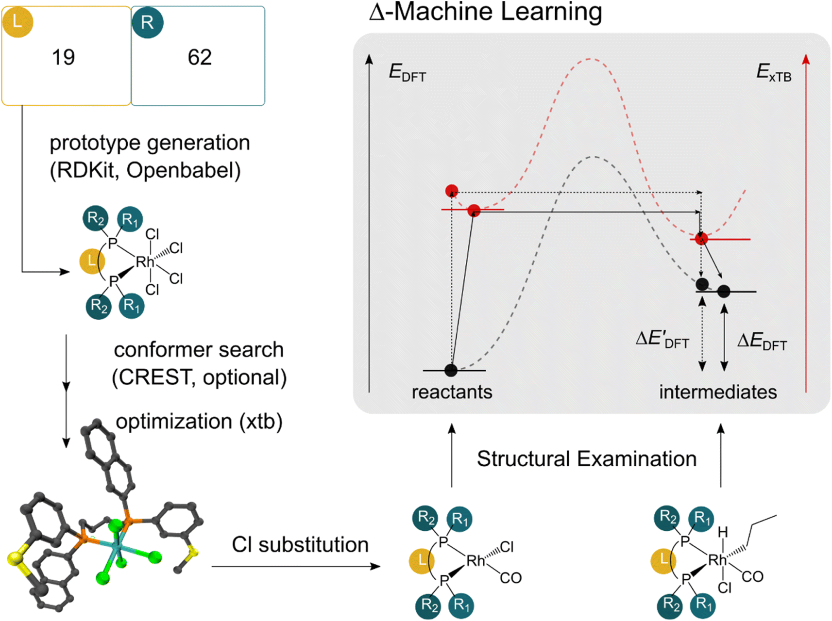

Fig. 2 Computational protocol used in the generation of the DFT and xTB data. We first employ RDKit and OpenBabel to generate fictitious prototypic species with 4 Cl ions in a combinatorial manner. A conformer search using CREST is employed on a subset of prototypes. All conformers of the prototype were considered as distinct complexes in the data set. A subsequent xTB optimization was employed on all prototypic species before the substitution of the Cl ions to obtain the reactant and intermediate species.

The geometry guesses required to optimize the reactant and intermediate states were generated using a combination of RDKit (2022.03)⁴⁵ and OpenBabel (3.0).⁴⁶ We initiated the construction of reactants and intermediates geometries from an octahedral Rh(PLP)(Cl)₄ prototype, where the linkers L, as well as the residual groups R₁ and R₂ were selected from a comprehensive set of 19 different linkers and 62 residual groups (see Fig. S5†). To address potential conformational variations, conformer searches using CREST⁴⁷ were performed within a subset of prototypes. In addition to the conformer with the lowest energy, several other minima on the xTB potential energy (hyper)surface (PES) were identified in the conformer search processes. Each of these minima represented different prototypic molecules, and would subsequently serve as individual data points for ML analysis.

After the prototypes were optimized at GFN2-xTB (6.6.1)³⁴ level of theory, the initial guesses of 4-coordinated reactants Rh(PLP)(Cl)(CO) were achieved by removing the excess chloride ions in the axial positions. Furthermore, one additional chloride ion in the equatorial plane is replaced by CO. Additionally, the initial geometries of 6-coordinated intermediates Rh(PLP)(Cl)(CO)(H)(propyl) were generated by substituting one chloride ion in the axial position with H, and two equatorial chloride ions with a propyl group and a CO, respectively.

Calculations at density functional of theory (DFT), as well as at xTB level of theory, were carried out sequentially for every system, to obtain the target values ΔE_DFT and , as well as the baseline values ΔE_xTB and for our ML objectives.

Firstly, xTB optimizations were performed on the initial guesses of reactants and intermediates, yielding the xTB single point energies E_xx,r and E_xx,i. Subsequently, both xTB-optimized species were further optimized at the level of DFT, yielding the single-point DFT energies E_DD,r and E_DD,i, respectively.

The DFT calculations, employing the range-separated ωB97XD functional⁴⁸ and the def2-SVP basis set, along with the respective effective core potential,⁴⁹ were carried out in the Gaussian 16 software package.⁵⁰ A vibrational analysis was carried out for DFT-equilibrium structures to verify that a minimum was obtained on the PES. Furthermore, the DFT single-point energies E_xD,i, were obtained by performing a calculation for each xTB-optimized intermediate while the xTB single-point energies E_Dx,r, were obtained for each DFT-optimized intermediate. Recall that E_xD,i is used to calculate the target upper bound of reaction energy (eqn (2)), and E_Dx,r is used to calculate the corresponding baseline value (eqn (3)). Structural assessments were performed on reactants and intermediates optimized at both DFT and xTB levels of theory, to validate that the coordination numbers of Rh ion are 4 and 6 in reactant and intermediate states, respectively. In addition, the phosphine ligands of both reactant and intermediate states of the molecules are ensured to be in cis-position.

2.4. Machine learning models trained on the ACs, AIM-ACs and SOAPs

After examining the structure of the reactants and intermediates, three sets of feature vectors based on ACs, AIM-ACs, and SOAPs of complexes were calculated for the Δ-ML study. To decrease the training time and complexity⁵¹ for the non-linear model, a feature selection based on an extra-trees regressor,⁵² as implemented in scikit-learn,⁵³ was performed to reduce the dimension of the feature vectors. In this selection method, the extra-tree models were trained to predict and ΔE_DFT merely with the ACs, AIM-ACs or SOAPs features, i.e., in the absence of the and ΔE_xTB, respectively. The features with importance lower than 0.0003 were considered unimportant and discarded, and by this filtering, the dimensionality of the feature vectors was considerably decreased. The dimensionalities of the various feature sets before and after reduction are summarized in Table S2.†

The artificial neural network (ANN) implemented within the NeuralFastAI⁵⁴ framework, was employed to train the two types of Δ-ML models on the features after dimensionality reduction. The ANN models utilize the rectified linear functions (ReLU) to capture potential nonlinear relationships between the features on the target values. For optimization, the Adam optimizer,⁵⁵ a method for efficient stochastic optimization, was employed to fit the parameters of the model. Hyperparameters, including the network architectures, embedding layers dropout rate, linear layers dropout rate, and number of epochs were optimized efficiently using the Bayesian optimization^56,57 in an automated fashion, as implemented in the AutoGluon package (1.0).⁵⁸ Other classical ML models, such as XGBoost⁵⁹ and CatBoost,⁶⁰ are also available in the AutoGluon package and can be implemented conveniently in an automated fashion as well.

Furthermore, the permutation importance^61,62 of the features was assessed on the best-performing model, in order to gain insights into the relationships between the descriptors and the deviation of the baseline values from the target values.

3. Results and discussion

3.1. Predictions on the upper bound of reaction energy

In this study, 1743 reactant–intermediate pairs were successfully optimized, and the corresponding target values and ΔE_DFT were obtained. Fig. 3a provides a visual representation of the disparity between the baseline model and the target model, where the baseline values range from −96.6 to 121.4 kJ mol⁻¹ while the target values range from 59.7 to 298.9 kJ mol⁻¹. Directly applying linear regression to the baseline values for predicting the target values yields significant errors, with a root mean squared error (RMSE) of 23.2 kJ mol⁻¹ and a coefficient of determination (R²) of only 0.55. This deviation of baseline and target values is exclusively introduced by the disparities stemming from the choice of different calculation levels.

Fig. 3 Parity plots between baseline value and target value: (a) between and , and (b) between ΔE_xTB and ΔE_DFT. A linear regression fit between the baseline values and target values was performed on the 1743 reactant–intermediate pairs, yielding a correlation R² of 0.541 and 0.563, respectively.

To account for the difference arising from the different calculation levels, -models were trained using AIM-ACs and ACs of varying depths as molecular descriptors. The dataset of 1743 reactant–intermediate pairs were split into training, validation and test sets with a ratio of 64 : 16 : 20 in two steps: first, 20% of the total data were randomly selected to form the test set for all models in our study. The remaining data were randomly split into training and validation set with a ratio of 8 : 2 (64% and 16% of all data, respectively) during the automated training procedure as implemented in the Autogluon package.⁵⁸ The performance of the -models is depicted in Fig. 4. Having comprised the electron information computed at both DFT and xTB levels of theory, all models trained on AIM-ACs with varying maximum depths d_max exhibited notably good performance, with a RMSE of approximately 11.0 kJ mol⁻¹ and a R² exceeding 0.90. When increasing the maximum feature depth from 1 to 3, the RMSE decreased from 11.1 kJ mol⁻¹ to 10.6 kJ mol⁻¹, and the R² increased from 0.905 to 0.913. The optimal performing model, achieved with d_max = 3, had 4 hidden layers with 1042, 367, 150, 121 neurons, respectively, along with an embedding layer dropout rate of 0.651, linear layer dropout rate of 0.002 and 24 epochs. The hyperparameter sets and other detailed results of the optimal models trained on different d_max are summarized in Table S2.† Besides the ANN models, the identical training set was also fed to other models, such as XGBoost⁵⁹ and CatBoost.⁶⁰ The results for these models are summarized in Table S3.† The performance of the ANN model is slightly better than these classical ML models. Therefore, we mainly focus on the discussion of the performance of ANN models throughout this study. Further increasing the maximum feature depth did not improve the performance of the -models. This suggests that the discrepancy between and can be attributed to the difference in description of electron information in the short range (d = 0, 1, 2, 3). Fig. 4c provides insight into the fraction of AIM-ACs with different d_max after dimensionality reduction. As d_max increased from 3 to 9, the fraction of AIM-ACs of d = 0, 1, 2, 3 remained consistently over 0.72. This observation supports the conclusion that including AIM-AC features with larger d_max (d_max > 3) does not provide additional information for addressing the difference between and .

Fig. 4 Performance of -model for predicting the target using AIM-ACs and ACs as features. Plot (a) and (b) depict the variation of root mean squared error (RMSE) and the coefficient of determination (R²) as functions of the maximum number of depths d_max. Dimensionality reduction was performed on both feature sets before training. Plot (c) and (d) illustrate the change of distribution of AIM-ACs and ACs of different depths as the maximum depth, d_max, changes.

Although -models trained on AIM-ACs have exhibited excellent performance, it is important to note that the calculations for AIM-based atomic properties are computationally demanding, rendering AIM-ACs less practical in accelerating high-throughput screening for the desired catalysts. In contrast, the original ACs based on the isolated atomic properties demand significantly lower computational costs.

In our study, a substantial number of isolated atomic properties derived from DFT calculations with a ωB97XD functional⁴⁸ and the parameters used in xTB calculations were used to construct the ACs (see ESI†). However, in comparison to AIM-ACs, the -models trained on ACs generally had poorer performance in predicting the . The best performing model was obtained at d_max = 7, with a RMSE of 14.2 kJ mol⁻¹ and a R² of 0.845. Fig. 4d illustrates the importance of including the atomic properties with larger d_max. As d_max increased from 1 to 7, the peak of the fraction also moves towards a higher d values, with d = 5 and d = 6 contributing the largest fraction (0.23 and 0.24, respectively) to the entire feature vector. On the contrary, ACs of d = 0 and d = 1 were less important and discarded via the dimensionality reduction procedure as d_max increased.

The details of the best performing models trained on AIM-ACs (d_max = 3) and ACs (d_max = 7), along with the corresponding feature importance analysis, are presented in Fig. 5. Regarding the model trained on AIM-ACs with d_max = 3, data points in the test and training sets were distributed evenly around the y = x line in the parity plot. Compared to the prediction performance using the pure baseline value (as shown in Fig. 3a), this -model displays a notable enhancement, with the RMSE decreasing from 23.2 to 10.6 kJ mol⁻¹. Feature importance analysis indicates that the a-AIM-ACs contributed the most to the improvement, among a total of 364 features. On the contrary, the l-AIM-ACs, which are designed to describe the ligands, play less crucial roles in improving the model. Although this optimal model was trained on the AIM-ACs with d_max = 3, features of d = 0 and 1 exhibited the strongest predictive power, with AIM-ACs of d = 2, 3 contributing only minor corrections to the model.

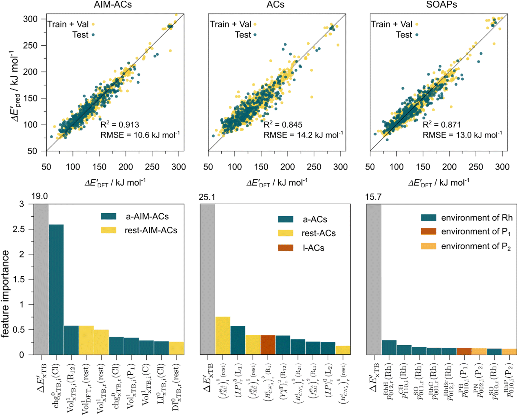Fig. 5 Parity plots between the prediction values and the true (DFT) values of the best -models trained on AIM-ACs (d_max = 3), ACs (d_max = 7) and SOAPs feature sets, respectively, as well as the corresponding feature importance analysis.

Compared to AIM-ACs, -model trained on ACs exhibited lower accuracy, and notable deviating points were observed in both test and training sets. This disparity could be attributed to the inherent inflexibility of ACs compared to AIM-ACs, as the distribution of ACs in is much sparser than that of AIM-ACs. Nevertheless, when compared to the pure baseline model, the performance of the -model trained on ACs has substantially improved at a considerably lower cost. In contrast to the model trained on AIM-ACs, the ACs of d = 0 or d = 1 barely provided distinctive information for different complexes. Consequently, ACs of greater depth (d = 2 ∼ 6) have higher predictive power in addition to the baseline value 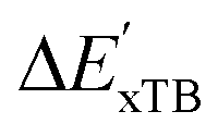. It is noteworthy that the features with high importance are dependent on the xTB parameters, particularly the anisotropic XC scaling parameter f_XC^θ_A, which is parametrized to describes the quadrupole expansion of the electron density of a specific element and account for the anisotropic exchange-correlation effect.³⁴

In addition to the topology-based features such as AIM-ACs and ACs, the -model was also trained on the position-based feature set, such as SOAPs, which can be computed very efficiently in the describe^43,44 package. Compared to the model trained on ACs, the model trained on SOAPs exhibited superior prediction performance, with a RMSE of 13.0 kJ mol⁻¹ and a R² of 0.871. The optimal set of hyperparameters is summarized in Table S2.† In contrast to the model trained on AIM-ACs features, where the xTB charge of the Cl ion in the intermediate (chg⁰_xTB(Cl)) emerged as the most important feature, the atomic environments around Rh (p(Rh)) played the most significant role among a total of 463 features, in enhancing the predictive performance of the model trained on SOAPs.

In summary, the -models trained on AIM-ACs exhibit strong predictive performance. However, it is important to note that the calculation of the AIM properties demands high computational power (roughly equivalent to a single point calculation), due to the heavy numerical integration of the electron density. Nevertheless, by comprising the electron information into the feature sets, these models point out that the charge in the Cl basin calculated at the xTB level of theory (chg⁰_xTB(Cl)) is the most relevant feature accounting for the difference between and . Alternatively, ACs and SOAPs provide a much faster route to predict with relatively high accuracies. In the case of ACs, features with higher d value have stronger predictive power while in the case of SOAPs, the atomic environments of Rh play significant roles in enhancing the performance of the model.

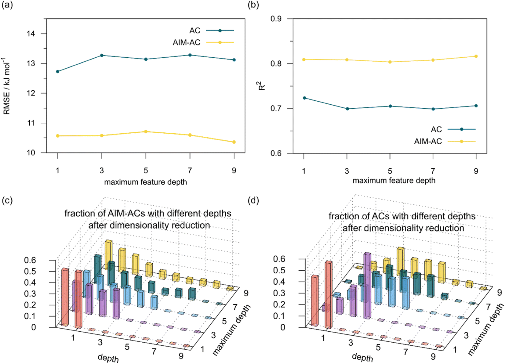
3.2. Predictions on the reaction energy ΔE_DFT

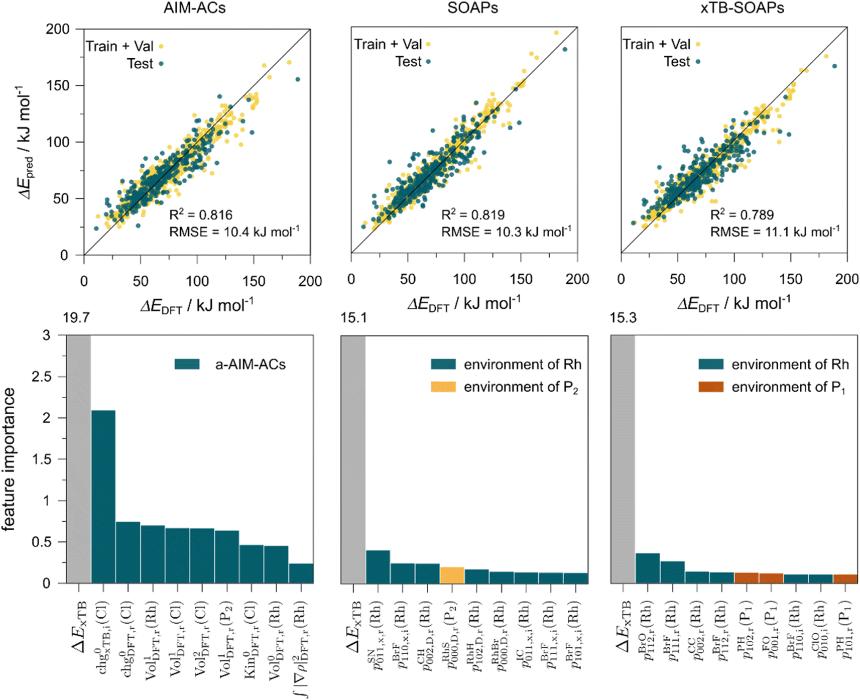
The Δ-ML strategy has been further adapted to predict the reaction energy ΔE_DFT, which plays a significant role in determining the relative concentration of the intermediate and reactant in equilibrium. Therefore, finding a suitable ligand architecture that can reduce the reaction energy ΔE_DFT would be advantageous for facilitating the C–H activation and subsequent functionalization. Fig. 3b illustrates the difference between the baseline values ΔE_xTB and the target values ΔE_DFT, where the values span from of −66.8 to 167.0 kJ mol⁻¹, and from 10.8 to 205.5 kJ mol⁻¹, respectively. The results of Δ^D_x-models trained on AIM-ACs and ACs with different d_max values are presented in Fig. 6. The best performing models were achieved when trained on d_max = 9 and d_max = 1, with RMSEs of 10.4 and 12.5 kJ mol⁻¹, respectively. However, compared to corresponding the -models, Δ^D_x-models exhibited lower R² values, which suggests that the features have a limitation in predicting the difference between ΔE_DFT and ΔE_xTB. This arises from two aspects, the different levels of theory and the changes in geometries. In addition to the information provided by AIM-ACs of d = 0, 1, 2, 3, which mainly accounts for the difference in calculation levels (as discussed in Section 3.1), including the information of greater depths can further enhance the performance of the model. The proportion of AIM-ACs of d = 7, 8, 9 is also comparably larger in this model than in the -model, with a fraction of 0.11 vs. 0.02, respectively (refer to Fig. 6cvs.Fig. 4c). The presence of non-zero AIM-AC features of greater depth (d = 7, 8, 9) typically suggests that the complex possesses a large and bulky ligand, which may introduce more significant deviation between the xTB- and DFT-equilibrium structures. Therefore, including the AIM-ACs of greater depths can potentially account for the difference due to the change in geometries.

Fig. 6 Performance of Δ^D_x-model for predicting the target ΔE_DFT using AIM-Acs and Acs as features. Plot (a) and (b) depict the variation of root mean squared error (RMSE) and the coefficient of determination (R²) as functions of the maximum number of depths d_max. Dimensionality reduction was conducted on both feature sets before training. Plot (c) and (d) illustrate the changes of distribution of AIM-Acs and Acs of different depths as the maximum depth, d_max, changes.

The Δ^D_x-models trained on ACs generally exhibit lower accuracies than the models trained on AIM-ACs. Unexpectedly, the best performing model was obtained at d_max = 1, with a RMSE of 12.7 kJ mol⁻¹ and a R² of 0.723. Fig. 6d illustrates that the fraction of ACs of d = 0, 1 dropped drastically as d_max increases. However, in contrast to the prediction, including the AC features with d > 1 does not improve the accuracy of the model.

Details and the feature importance analysis of the Δ^D_x-model trained on AIM-ACs with d_max = 9 are shown in Fig. 7. Data points in the test and training sets were distributed uniformly around the y = x line in the parity plot, with only a few notably deviating points present in the high energy region where ΔE_DFT exceeds 100 kJ mol⁻¹. The corresponding feature importance analysis reveals that a-AIM-ACs are the most significant contributors to the high predictive performance of the model. Among these features, the electron information around Cl and Rh ions are of the highest significance among a total of 507 features, particularly the AIM-charge of Cl in the intermediate calculated at xTB level of theory (chg⁰_xTB,i(Cl)). As discussed in Section 3.1, this feature primarily accounts for the difference arising from the different calculation levels of theory. In contrast to the -model, where electronic information from xTB calculations plays a more prominent role, DFT information from the reactant is more important in this model, in addition to the already known importance of chg⁰_xTB,i(Cl). Note that the changes in geometries in both reactants and intermediates can introduce errors independently to the prediction in the energy difference. The structural change of the reactants can be captured by the AIM analysis on the DFT-equilibrium structure and xTB-equilibrium structure of the reactant, namely, on R_DFT,r and R_xTB,r, respectively. However, the change in geometries of the intermediates remains hard to describe solely through the AIM analysis of R_xTB,i. Therefore, higher importance of the AIM-ACs which depend on the DFT calculations is observed. On the contrary, it is less practical to discuss the results for Δ^D_x-models trained on ACs due to their low prediction accuracy. Nevertheless, the parity plot and the corresponding feature importance ranking are shown in Fig. S6.†

Fig. 7 Parity plots between the prediction values and the true (DFT) values of the best Δ^D_x-models trained on AIM-ACs (d_max = 9), SOAPs and SOAPs feature only depending on xTB structures (xTB-SOAPs), respectively, as well as the corresponding feature importance analysis.

Furthermore, the Δ^D_x-model was trained using SOAPs that depend on the structure of reactants optimized at both xTB and DFT levels of theory, as well as the structure of the intermediate optimized at the xTB level of theory. It is noteworthy that SOAPs can be calculated much more efficiently compared to AIM-ACs, and the performance of the model trained on these features even slightly exceeds that of the model trained on AIM-ACs, with a RMSE of 10.3 kJ mol⁻¹ and a R² of 0.819. Given that SOAPs are less accurate in predicting the difference in different levels of theory than the AIM-ACs, as demonstrated in the comparative study on the -models, this result suggests that SOAPs may have stronger predictive power regarding the change in geometries. Among all the SOAP features, the atomic environment of the Rh ions in DFT-equilibrium structures of the reactants and in xTB-equilibrium structures of the intermediates is the most significant factor for the accuracy of this Δ^D_x-model.

The SOAPs can be further simplified by excluding the information of the DFT structure, although it plays an important role according to the results of the feature ranking. In this manner, the energy difference of the reaction obtained at the DFT level of theory ΔE_DFT can be predicted exclusively using the information from xTB calculations, which eliminates the need for computationally expensive structural optimizations at the DFT level of theory. This simplified feature set is denoted as xTB-SOAPs. The DFT calculation for a molecule containing 72 atoms typically requires more than two days of CPU time, while a xTB optimization for the same molecule requires less than one minute on the same machine. In addition, the generation of the SOAP features requires less than one second. In general, xTB-SOAPs can be generated very efficiently. Note that xTB-SOAPs only gain efficiency in predicting ΔE_DFT but not . This is due to the fact that xTB-SOAPs and SOAPs are identical for the prediction of , since the energies of the complexes at xTB and DFT levels were evaluated for identical geometries. As expected, the performance of the Δ^D_x-model slightly deteriorated after excluding the information from DFT-equilibrium structures, with the RMSE increasing to 11.1 kJ mol⁻¹, and the R² reducing to 0.789. However, compared to the prediction from pure baseline values ΔE_xTB, this is already a considerable improvement with only a minor increase in computational cost. Although this result is less accurate than the predictive study of activation energies of different types of elementary reactions,^23,24,28 where the errors range from 2.0 to 8.1 kJ mol⁻¹, our study allows the prediction of energy differences between the reactant and intermediate. The structural difference between the reactant and the intermediate is greater than the difference between the reactant and the TS, because they are further apart on the 3N-6 potential energy surface. This could be the reason for the difficulties in predicting the reaction energy.

Without the information of the atomic environments of Rh obtained in the DFT-equilibrium structure, the feature ranking shows an increased importance of the environment around P₁ in the reactant, which emphasizes information from the ligands. A large size and high bulkiness of a ligand usually implies a large deviation between DFT-equilibrium and xTB-equilibrium structures. Therefore, the importance of a more detailed description on the ligand structure is heightened, when the direct descriptions on the change in geometries, such as SOAPs evaluated on DFT-equilibrium structure, are absent.

In summary, the Δ^D_x-model trained on AIM-ACs and SOAPs exhibits good performance in predicting the energy difference ΔE_DFT. However, these two feature sets may account for different aspects of the difference between the baseline value and the target value: AIM-ACs are more related to the difference in levels of theory, while SOAPs are more associated to the change in geometry. Furthermore, xTB-SOAPs features are highly recommended for efficient prediction of the energy difference, owing to the low computational costs for xTB optimization and SOAPs calculation.

3.3. High-throughput screening using the Δ^D_x-model trained on xTB-SOAPs

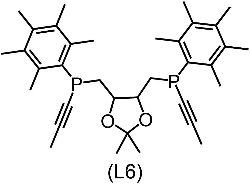
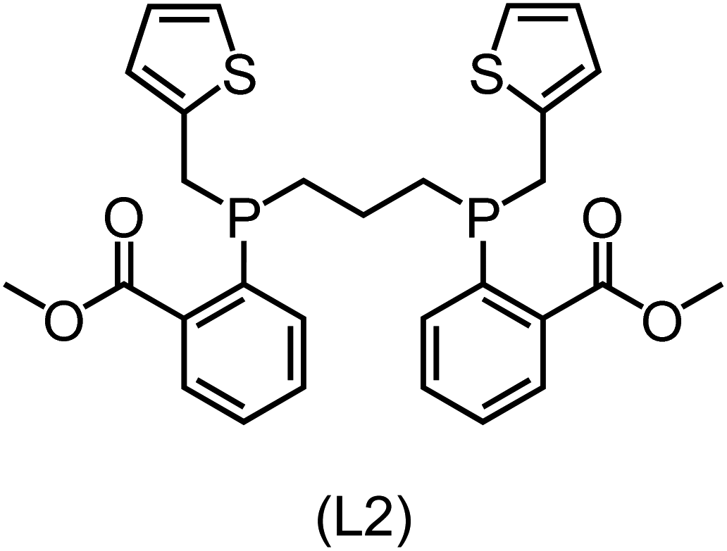
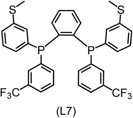
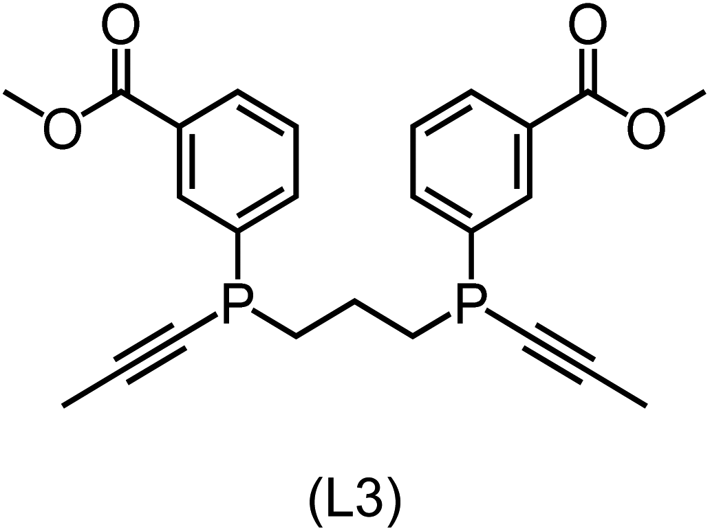
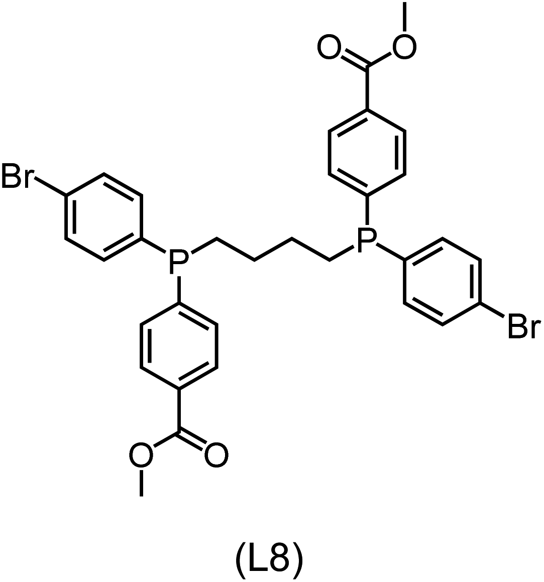
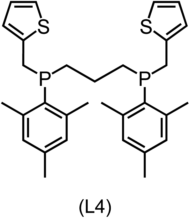
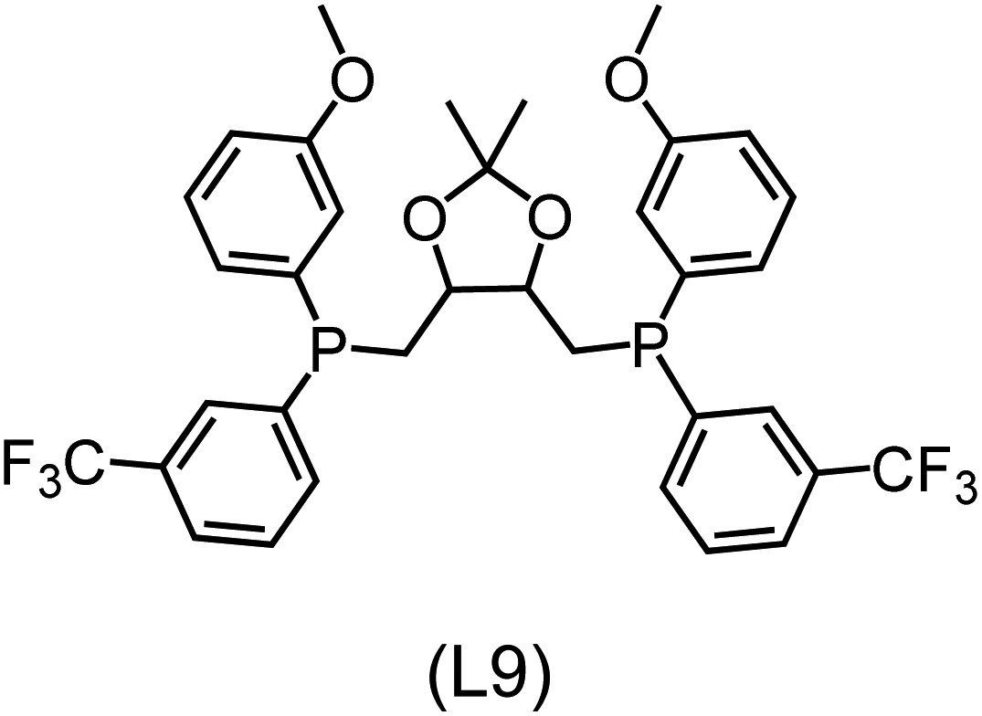
Utilizing the Δ^D_x-model trained on xTB-SOAPs, we propose an efficient two-step screening pipeline for exploring the chemical space of Rh complexes featuring bidentate phosphine ligands. First, 27 832 selected reactant and intermediate pairs undergo xTB optimization without conformer search. The baseline value ΔE_xTB, as well as the SOAP features were evaluated at the xTB equilibrium structure of reactants and intermediates. After the evaluation of ΔE_ML using the trained Δ^D_x-model, 60 pairs with lowest reaction energies are selected for a refined screening step. In a second step, the selected reactant–intermediate pairs undergo conformer search. ΔE_ML and SOAP features were obtained from the corresponding optimal conformer structures. Detailed information on the procedure is described in the ESI.† Implementing the two-step high-throughput screening procedure onto a vast chemical space with 27 832 data points, we identified ten reactant–intermediate pairs of Rh complexes with potentially the lowest ΔE_ML. These Rh complexes are promising catalysts for the C–H activation process. The Lewis structures of the bidentate phosphine ligands, the predicted energy difference of the reactant–intermediate pairs ΔE_ML, the baseline value ΔE_xTB, as well as the target value ΔE_DFT as validation, are summarized in Table 1. The related activation energies and isomerization energies of the 6-coordinated intermediates are summarized in Table S5.† The RMSE evaluated on these 10 reactant–intermediate pairs is 10.8 kJ mol⁻¹, where the errors of six of these structures are smaller than 5.0 kJ mol⁻¹. Compared to the averaged reaction energy of the original dataset with 1743 data points (68.0 kJ mol⁻¹), the average reaction energy of the ten newly proposed structures is 34.8 kJ mol⁻¹ lower (33.2 kJ mol⁻¹). In addition, the relationship between the activation energy and reaction energy of the reactant–intermediate pairs is demonstrated in Fig. 8. As expected, the reaction energy (ΔE_DFT) and activation energy (ΔE^‡_DFT) are highly correlated. Compared to the 16 structures in our previous mechanistic study,³⁰ the ten new structures have not only a lower ΔE_DFT (33.2 vs. 61.8 kJ mol⁻¹) but also a lower ΔE^‡_DFT (108.3 vs. 133.6 kJ mol⁻¹). This outcome indicates that the Δ^D_x-model trained on xTB-SOAPs provides an efficient and reliable way for searching complexes with low reaction energies, which usually possess low activation energy as well. Recalling that the C–H activation is one of the rate-determining steps in an alkane carbonylation reaction as we have shown previously,³⁰ our screening pipeline is effective in designing ligand structures with high catalytic efficacy.

Table 1 Details of the 10 reactant–intermediate pairs with lowest ΔE_ML selected from the two-step screening procedure, including the structure of the ligands, the predicted energy difference ΔE_ML, the baseline value ΔE_xTB (in squared bracket) and the target value ΔE_DFT (in parentheses) as validation

Ligand structure (label)	ΔEML (ΔEDFT) [ΔExTB]/kJ mol^−1	Ligand structure (label)	ΔEML (ΔEDFT) [ΔExTB]/kJ mol^−1
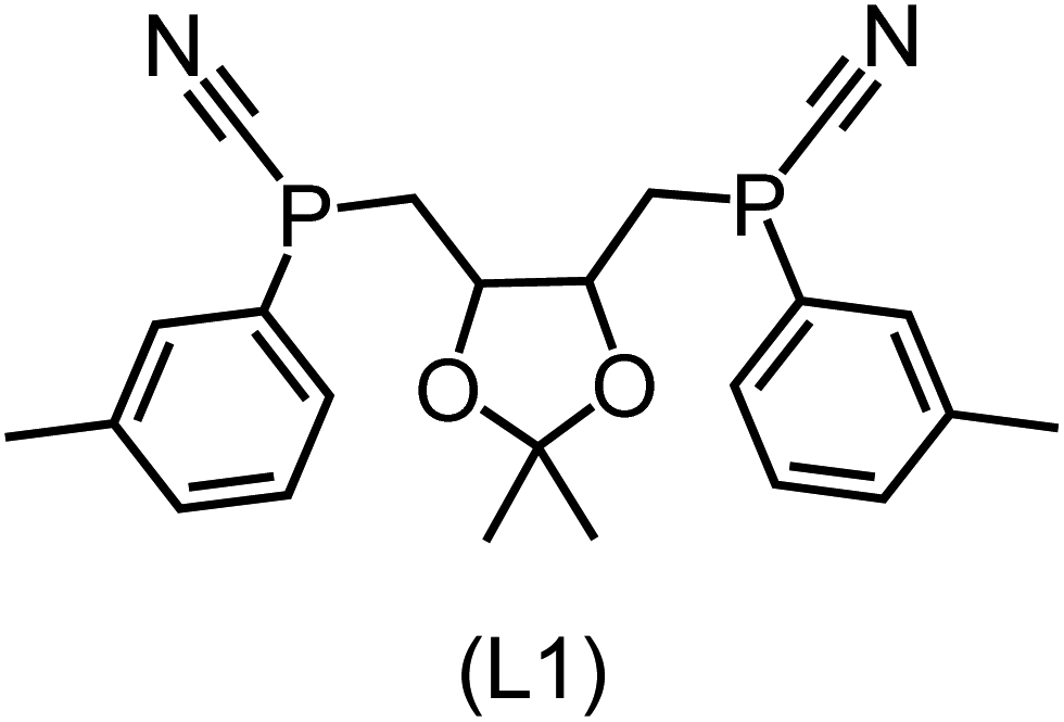
	19.1 (21.9) [−25.8]		27.7 (41.3) [5.4]
	19.9 (44.2) [11.4]		31.7 (27.1) [−22.3]
	22.6 (19.8) [−31.6]		33.7 (31.5) [−9.2]
	23.3 (36.2) [−9.9]		33.9 (38.2) [−0.1]
	24.5 (25.4) [−5.9]		34.2 (46.7) [−5.8]

---

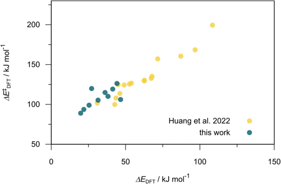Fig. 8 Relationship between the reaction energy (ΔE_DFT) and activation energy ΔE^‡_DFT of C–H activation. Compared to the 16 structures from our previous study,³⁰ the ten newly selected structures possess lower reaction energies as well as lower activation energies.

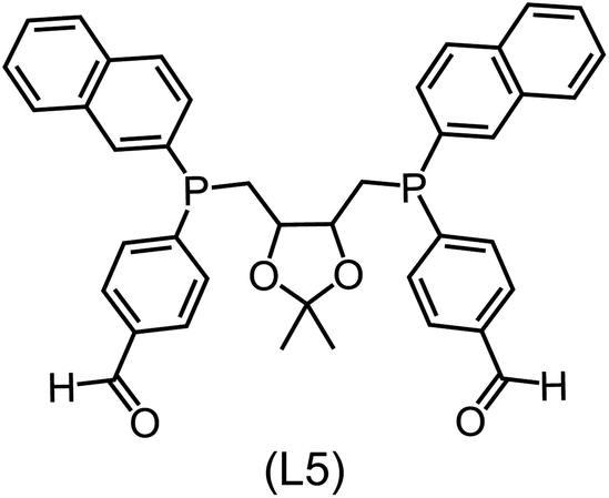
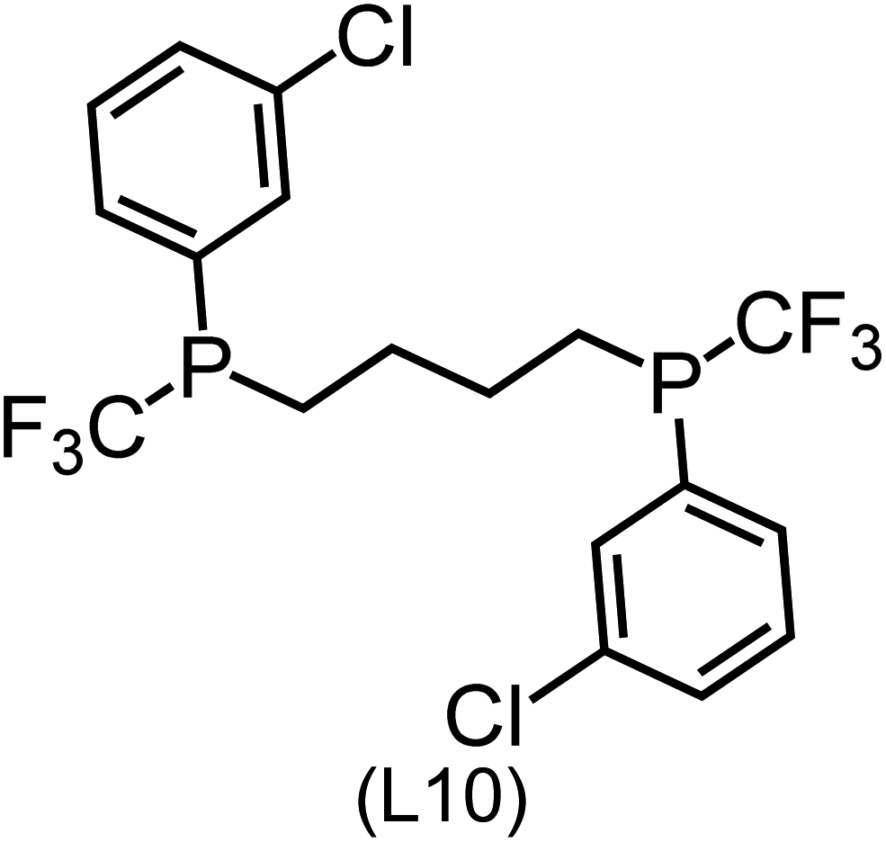
Regarding the structures of the ligands of the ten selected complexes, as can be seen from Table 1, the linker unit connecting the two coordinating phosphorous atoms varies and includes flexible alkyl chains but also more rigid aromatic or 2,3-O-isopropylidene-2,3-dihydroxy-1,4-bisbutyl structures. All structures have in common that the phosphorus atoms bear at least one aromatic substituent. A more in-depth analysis of geometric and electronic parameters based on the DFT-optimized [Rh(PLP)(CO)(Cl)] equilibrium structures reveals that the newly suggested ligand structures have larger buried B5 Sterimol parameters,⁶³ as well as an on average lower dipole moment. In total 20 geometric and electronic descriptors exhibit significant differences between the original and the newly proposed bisphosphine set (see ESI†). Importantly, steric factors describing the accessibility of the Rh center such as the % buried volume⁶⁴ are included in this descriptor set. The complexes with a lower predicted reaction energy also have a lower % buried volume, pointing to the fact that the Rh center is more accessible for the substrate. Overall, the dependence of the C–H activation reaction energy on the complex structure cannot be explained with a single factor, instead, multiple geometric and electronic parameters influence the C–H activation process. This underlines the complexity when searching for new C–H activation catalysts.

When looking at the synthetic accessibility of the suggest structures it can be concluded that although the ligands look complex at first, the structures can be realistically synthezised as both the linker as well as the substituted phosphine part can be independently synthezised. E.g. the 2,3-O-isopropylidene-2,3-dihydroxy-1,4-bisbutyl linker found in L1, L5, L6 and L9 can be synthezised following the procedure from Kagan and Dang,⁶⁵ while the unsymmetric phosphines can be synthesized following Singh and Nicholas.⁶⁶ Thus, the structures suggested in Table 1 can be synthezised and subsequently their performance can be experimentally validated.

4. Conclusion

In this study, an efficient and reliable prediction of the energy difference between the 4-coordinated Rh(PLP)(CO)(Cl) and 6-coordinated Rh(PLP)(CO)(Cl)(H)(propyl) was realized by employing the Δ-ML approach. On the one hand, the -model trained on autocorrelation functions based on atoms in molecules theory (AIM-ACs) achieved the best performance with a root-mean-squared error (RMSE) of 10.6 kJ mol⁻¹ and a R² of 0.913. This result underscores the superiority of AIM-ACs over the other two feature sets in accounting for errors due to the difference in the level of theory. On the other hand, the Δ^D_x-model trained on smooth overlap atomic position (SOAP) features achieved remarkable performance with an RMSE of 10.3 kJ mol⁻¹ and an R² of 0.819, which suggests that SOAPs have better performance in accounting for errors due to the change in geometry. Notably, the Δ^D_x-model trained on xTB-SOAPs alone excels not only in efficiently screening the chemical space of Rh complexes featuring bidentate phosphine ligands but also in accurately predicting the reaction energies ΔE_DFT. With our approach, we were able to predict ten promising ligand structures that should feature a low C–H reaction energy and therefore, should be able to substantially accelerate the catalytic functionalization of alkanes.

Data availability

The DFT optimized xyz files, the Gaussian16 log files as well as csv files used for training of the different models are available from Zenodo (https://doi.org/10.5281/zenodo.10529636, DOI: 10.5281/zenodo.10529636, Version used: 1.0). Additional detailed experiment descriptions, figures, as well as tables supporting the findings of the article can be found in the ESI.†

Author contributions

R. G., A. C. and S. G. performed the conceptualization and the project-administration. T. H. and R. G. performed quantum chemical simulations, data analysis and machine learning. Figures and the original draft were prepared by T. H. All authors contributed to the writing by reviewing and editing of the original draft.

Conflicts of interest

The authors declare no conflict of interest.

Acknowledgements

T. H. and S. G. gratefully acknowledge funding from Carl-Zeiss-Stiftung “Durchbrüche”. S. G. highly acknowledges funding by the German Science Foundation DFG within the priority program SPP 2363 “Molecular Machine Learning”, GR4482/6. R. G. gratefully acknowledges funding from the “Bund-Länder Tenure-Track Programm” of the Federal Ministry of Education and Research (BMBF) as well as by an accompanying grant from the Free State of Thuringia (FKZ: 16TTP133). The major part of the calculations were performed at the Universitätsrechenzentrum of the Friedrich Schiller University Jena, while a minor part was performed at TU Ilmenau.

References

1. W.-H. Wang, Y. Himeda, J. T. Muckerman, G. F. Manbeck and E. Fujita, CO2 Hydrogenation to Formate and Methanol as an Alternative to Photo- and Electrochemical CO2 Reduction, Chem. Rev., 2015, 115, 12936–12973.
2. R. Crabtree, Iridium compounds in catalysis, Acc. Chem. Res., 1979, 12, 331–337.
3. M. D. Kärkäs, O. Verho, E. V. Johnston and B. Åkermark, Artificial Photosynthesis: Molecular Systems for Catalytic Water Oxidation, Chem. Rev., 2014, 114, 11863–12001.
4. T. Shen, Q. Xie, Y. Li and J. Zhu, Aromaticity-promoted C− F Bond Activation in Rhodium Complex: A Facile Tautomerization, Chem.–Asian J., 2019, 14, 1937–1940.
5. Y. Li and J. Zhu, Achieving a favorable activation of the C–F bond over the C–H bond in five-and six-membered ring complexes by a coordination and aromaticity dually driven strategy, Organometallics, 2021, 40, 3397–3407.
6. X. Li, W. Ouyang, J. Nie, S. Ji, Q. Chen and Y. Huo, Recent Development on Cp* Ir (III)-Catalyzed C− H Bond Functionalization, ChemCatChem, 2020, 12, 2358–2384.
7. T. Sakakura, T. Sodeyama, K. Sasaki, K. Wada and M. Tanaka, Carbonylation of hydrocarbons via carbon-hydrogen activation catalyzed by RhCl (CO)(PMe3) 2 under irradiation, J. Am. Chem. Soc., 1990, 112, 7221–7229.
8. A. J. Kunin and R. Eisenberg, Photochemical carbonylation of benzene by iridium (I) and rhodium (I) square-planar complexes, Organometallics, 1988, 7, 2124–2129.
9. K. J. Laidler and M. C. King, The development of transition-state theory, J. Phys. Chem., 1983, 87, 2657–2664.
10. A. L. Dewyer, A. J. Argüelles and P. M. Zimmerman, Methods for exploring reaction space in molecular systems, Wiley Interdiscip. Rev.: Comput. Mol. Sci., 2018, 8, e1354.
11. L. J. Broadbelt, S. M. Stark and M. T. Klein, Computer Generated Pyrolysis Modeling: On-the-Fly Generation of Species, Reactions, and Rates, Ind. Eng. Chem. Res., 1994, 33, 790–799.
12. C. W. Gao, J. W. Allen, W. H. Green and R. H. West, Reaction Mechanism Generator: Automatic construction of chemical kinetic mechanisms, Comput. Phys. Commun., 2016, 203, 212–225.
13. D. Rappoport, C. J. Galvin, D. Y. Zubarev and A. Aspuru-Guzik, Complex chemical reaction networks from heuristics-aided quantum chemistry, J. Chem. Theory Comput., 2014, 10, 897–907.
14. S. Habershon, Sampling reactive pathways with random walks in chemical space: Applications to molecular dissociation and catalysis, J. Chem. Phys., 2015, 143, 094106.
15. M. Bergeler, G. N. Simm, J. Proppe and M. Reiher, Heuristics-guided exploration of reaction mechanisms, J. Chem. Theory Comput., 2015, 11, 5712–5722.
16. A. L. Dewyer and P. M. Zimmerman, Finding reaction mechanisms, intuitive or otherwise, Org. Biomol. Chem., 2017, 15, 501–504.
17. D. H. Valentine Jr and J. H. Hillhouse, Electron-rich phosphines in organic synthesis II. Catalytic applications, Synthesis, 2003, 2003, 2437–2460.
18. H. Altae-Tran, B. Ramsundar, A. S. Pappu and V. Pande, Low data drug discovery with one-shot learning, ACS Cent. Sci., 2017, 3, 283–293.
19. A. Mayr, G. Klambauer, T. Unterthiner, M. Steijaert, J. K. Wegner, H. Ceulemans, D.-A. Clevert and S. Hochreiter, Large-scale comparison of machine learning methods for drug target prediction on ChEMBL, Chem. Sci., 2018, 9, 5441–5451.
20. Y. J. Colón and R. Q. Snurr, High-throughput computational screening of metal–organic frameworks, Chem. Soc. Rev., 2014, 43, 5735–5749.
21. J. P. Janet and H. J. Kulik, Resolving transition metal chemical space: Feature selection for machine learning and structure–property relationships, J. Phys. Chem. A, 2017, 121, 8939–8954.
22. T. Lewis-Atwell, P. A. Townsend and M. N. Grayson, Machine learning activation energies of chemical reactions, Wiley Interdiscip. Rev.: Comput. Mol. Sci., 2022, 12, e1593.
23. S. Choi, Y. Kim, J. W. Kim, Z. Kim and W. Y. Kim, Feasibility of activation energy prediction of gas-phase reactions by machine learning, Chem.–Eur. J., 2018, 24, 12354–12358.
24. Q. Ye, Y. Zhao and J. Zhu, Probing the origin of higher efficiency of terphenyl phosphine over the biaryl framework in Pd-catalyzed CN coupling: A combined DFT and machine learning study, Artif. Intell., 2023, 1, 100005.
25. I. Ismail, C. Robertson and S. Habershon, Successes and challenges in using machine-learned activation energies in kinetic simulations, J. Chem. Phys., 2022, 157, 014109.
26. M. Evans and M. Polanyi, Inertia and driving force of chemical reactions, Trans. Faraday Soc., 1938, 34, 11–24.
27. F. Palazzesi, M. R. Hermann, M. A. Grundl, A. Pautsch, D. Seeliger, C. S. Tautermann and A. Weber, BIreactive: a machine-learning model to estimate covalent warhead reactivity, J. Chem. Inf. Model., 2020, 60, 2915–2923.
28. P. Friederich, G. dos Passos Gomes, R. De Bin, A. Aspuru-Guzik and D. Balcells, Machine learning dihydrogen activation in the chemical space surrounding Vaska's complex, Chem. Sci., 2020, 11, 4584–4601.
29. P. Margl, T. Ziegler and P. E. Bloechl, Reaction of methane with Rh (PH3) 2Cl: A dynamical density functional study, J. Am. Chem. Soc., 1995, 117, 12625–12634.
30. T. Huang, S. Kupfer, M. Richter, S. Gräfe and R. Geitner, Bidentate Rh (I)-Phosphine Complexes for the C− H Activation of Alkanes: Computational Modelling and Mechanistic Insight, ChemCatChem, 2022, 14, e202200854.
31. J. S. Bridgewater, T. L. Netzel, J. R. Schoonover, S. M. Massick and P. C. Ford, Time-Resolved Optical and Infrared Spectral Studies of Intermediates Generated by Photolysis of trans-RhCl (CO)(PR3) 2. Roles Played in the Photocatalytic Activation of Hydrocarbons1, Inorg. Chem., 2001, 40, 1466–1476.
32. R. Ramakrishnan, P. O. Dral, M. Rupp and O. A. Von Lilienfeld, Big data meets quantum chemistry approximations: the Δ-machine learning approach, J. Chem. Theory Comput., 2015, 11, 2087–2096.
33. Q. Zhao, D. M. Anstine, O. Isayev and B. M. Savoie, D2 machine learning for reaction property prediction, Chem. Sci., 2023, 14, 13392–13401.
34. C. Bannwarth, S. Ehlert and S. Grimme, GFN2-xTB—An accurate and broadly parametrized self-consistent tight-binding quantum chemical method with multipole electrostatics and density-dependent dispersion contributions, J. Chem. Theory Comput., 2019, 15, 1652–1671.
35. H. Wiener, Structural determination of paraffin boiling points, J. Am. Chem. Soc., 1947, 69, 17–20.
36. B. Hollas, An analysis of the autocorrelation descriptor for molecules, J. Math. Chem., 2003, 33, 91–101.
37. A. P. Bartók, R. Kondor and G. Csányi, On representing chemical environments, Phys. Rev. B, 2013, 87, 184115.
38. M. Ceriotti, M. J. Willatt and G. Csányi, in Handbook of Materials Modeling: Methods: Theory and Modeling, Springer, Cham, 2020, pp. 1911–1937.
39. J. Devillers, D. Domine, C. Guillon, S. Bintein and W. Karcher, Prediction of partition coefficients (log p oct) using autocorrelation descriptors, SAR QSAR Environ. Res., 1997, 7, 151–172.
40. R. Bader, Atoms in molecules: a quantum theoryOxford University Press, USA, 1994.
41. R. J. Boyd and C. F. Matta, The quantum theory of atoms in molecules: from solid state to DNA and drug design, Wiley-VCH Verlag GmbH & Co. KGaA, 2007.
42. T. Lu and F. Chen, Multiwfn: a multifunctional wavefunction analyzer, J. Comput. Chem., 2012, 33, 580–592.
43. L. Himanen, M. O. Jäger, E. V. Morooka, F. F. Canova, Y. S. Ranawat, D. Z. Gao, P. Rinke and A. S. Foster, DScribe: Library of descriptors for machine learning in materials science, Comput. Phys. Commun., 2020, 247, 106949.
44. J. Laakso, L. Himanen, H. Homm, E. V. Morooka, M. O. Jäger, M. Todorović and P. Rinke, Updates to the DScribe library: New descriptors and derivatives, J. Chem. Phys., 2023, 158, 234802.
45. G. A. Landrum, et al., RDKit: Open-Source Cheminformatics Software, version 2022_03_3.
46. N. M. O'Boyle, M. Banck, C. A. James, C. Morley, T. Vandermeersch and G. R. Hutchison, Open Babel: An open chemical toolbox, J. Cheminf., 2011, 3, 1–14.
47. P. Pracht, F. Bohle and S. Grimme, Automated exploration of the low-energy chemical space with fast quantum chemical methods, Phys. Chem. Chem. Phys., 2020, 22, 7169–7192.
48. J.-D. Chai and M. Head-Gordon, Long-range corrected hybrid density functionals with damped atom–atom dispersion corrections, Phys. Chem. Chem. Phys., 2008, 10, 6615–6620.
49. F. Weigend and R. Ahlrichs, Balanced basis sets of split valence, triple zeta valence and quadruple zeta valence quality for H to Rn: Design and assessment of accuracy, Phys. Chem. Chem. Phys., 2005, 7, 3297–3305.
50. M. J. Frisch, G. W. Trucks, H. B. Schlegel, G. E. Scuseria, M. A. Robb, J. R. Cheeseman, G. Scalmani, V. Barone, G. A. Petersson, H. Nakatsuji, X. Li, M. Caricato, A. V. Marenich, J. Bloino, B. G. Janesko, R. Gomperts, B. Mennucci, H. P. Hratchian, J. V. Ortiz, A. F. Izmaylov, J. L. Sonnenberg, D. Williams-Young, F. Ding, F. Lipparini, F. Egidi, J. Goings, B. Peng, A. Petrone, T. Henderson, D. Ranasinghe, V. G. Zakrzewski, J. Gao, N. Rega, G. Zheng, W. Liang, M. Hada, M. Ehara, K. Toyota, R. Fukuda, J. Hasegawa, M. Ishida, T. Nakajima, Y. Honda, O. Kitao, H. Nakai, T. Vreven, K. Throssell, J. A. Montgomery Jr, J. E. Peralta, F. Ogliaro, M. J. Bearpark, J. J. Heyd, E. N. Brothers, K. N. Kudin, V. N. Staroverov, T. A. Keith, R. Kobayashi, J. Normand, K. Raghavachari, A. P. Rendell, J. C. Burant, S. S. Iyengar, J. Tomasi, M. Cossi, J. M. Millam, M. Klene, C. Adamo, R. Cammi, J. W. Ochterski, R. L. Martin, K. Morokuma, O. Farkas, J. B. Foresman and D. J. Fox, Gaussian 16 Rev. C.01, Wallingford, CT, 2016.
51. I. Guyon and A. Elisseeff, An introduction to variable and feature selection, J. Mach. Learn. Res., 2003, 3, 1157–1182.
52. P. Geurts, D. Ernst and L. Wehenkel, Extremely randomized trees, Mach. Learn., 2006, 63, 3–42.
53. F. Pedregosa, G. Varoquaux, A. Gramfort, V. Michel, B. Thirion, O. Grisel, M. Blondel, P. Prettenhofer, R. Weiss and V. Dubourg, Scikit-learn: Machine learning in Python, J. Mach. Learn. Res., 2011, 12, 2825–2830.
54. J. Howard and S. Gugger, Fastai: A layered API for deep learning, Information, 2020, 11, 108.
55. D. P. Kingma and J. Ba: A method for stochastic optimization, arXiv, 2014, preprint, arXiv:1412.6980,  DOI:10.48550/arXiv.1412.6980.
56. B. Shahriari, K. Swersky, Z. Wang, R. P. Adams and N. De Freitas, Taking the human out of the loop: A review of Bayesian optimization, Proc. IEEE, 2015, 104, 148–175.
57. A. Klein, L. C. Tiao, T. Lienart, C. Archambeau and M. Seeger, Model-based asynchronous hyperparameter and neural architecture search, arXiv, preprint, arXiv: 2003.10865,  DOI:10.48550/arXiv.2003.10865.
58. N. Erickson, J. Mueller, A. Shirkov, H. Zhang, P. Larroy, M. Li and A. Smola: Robust and accurate automl for structured data, arXiv, preprint, arXiv: 2003.06505,  DOI:10.48550/arXiv.2003.06505.
59. J. H. Friedman, Greedy function approximation: a gradient boosting machine, Ann. Math. Stat., 2001, 1189–1232.
60. L. Prokhorenkova, G. Gusev, A. Vorobev, A. V. Dorogush and A. Gulin, CatBoost: unbiased boosting with categorical features, arXiv, preprint, arXiv: 1706.09516,  DOI:10.48550/arXiv.1706.09516.
61. A. Altmann, L. Toloşi, O. Sander and T. Lengauer, Permutation importance: a corrected feature importance measure, Bioinformatics, 2010, 26, 1340–1347.
62. L. Breiman, Random forests, Mach. Learn., 2001, 45, 5–32.
63. T. Gensch, G. dos Passos Gomes, P. Friederich, E. Peters, T. Gaudin, R. Pollice, K. Jorner, A. Nigam, M. Lindner-D’Addario and M. S. Sigman, A comprehensive discovery platform for organophosphorus ligands for catalysis, J. Am. Chem. Soc., 2022, 144, 1205–1217.
64. L. Falivene, R. Credendino, A. Poater, A. Petta, L. Serra, R. Oliva, V. Scarano and L. Cavallo, SambVca 2. A web tool for analyzing catalytic pockets with topographic steric maps, Organometallics, 2016, 35, 2286–2293.
65. H. B. Kagan and T.-P. Dang, Asymmetric catalytic reduction with transition metal complexes. I. Catalytic system of rhodium (I) with (-)-2, 3-0-isopropylidene-2, 3-dihydroxy-1, 4-bis (diphenylphosphino) butane, a new chiral diphosphine, J. Am. Chem. Soc., 2002, 94, 6429–6433.
66. S. Singh and K. M. Nicholas, A novel synthesis of unsymmetrical tertiary phosphines: selective nucleophilic substitution on phosphorus (III), Chem. Commun., 1998, 149–150.

---

Footnote

† Electronic supplementary information (ESI) available. See DOI: https://doi.org/10.1039/d4dd00037d

---