 Open Access Article
Infrared spectra prediction using attention-based graph neural networks†
Naseem
Saquer
 a,
Razib
Iqbal
 *b,
Joshua D.
Ellis
b and
Keiichi
Yoshimatsu
 *a
*a
aDepartment of Chemistry and Biochemistry, Missouri State University, 901 South National Avenue, Springfield, MO 65897, USA. E-mail: KYoshimatsu@MissouriState.edu; Tel: +1 417 836 5613
bDepartment of Computer Science, Missouri State University, 901 South National Avenue, Springfield, MO 65897, USA. E-mail: RIqbal@MissouriState.edu; Tel: +1 417 836 4944
First published on 18th January 2024
Abstract
Infrared (IR) spectroscopy is an analytical technique that is used in broad disciplines of fundamental and applied research areas. Along those lines, it is of significant interest to develop an efficient computational method for the prediction of IR spectra based on chemical structures. In this work, we investigated the performance of attention-based graph neural networks. Our study showed that AttentiveFP model, which incorporates the message passing and graph attention mechanisms, exhibits the highest performance among the tested graph neural network models and a benchmark descriptor-based model. The implication is that the capability of AttentiveFP model to learn interactions between neighboring atoms and distant atoms allows for improving the performance of IR spectra prediction model. The mean Spearman correlation coefficient between the IR spectra predicted by AttentiveFP model and actual spectra was 0.911 and the correlation coefficient values were above 0.8 in 88% of the test cases. Our findings demonstrate the utility of the graph attention mechanism for the development of graph neural network-based machine learning models for IR spectra prediction with improved performances.
1 Introduction
Infrared (IR) spectroscopy is an analytical technique that is used in broad areas including chemical,1,2 materials,3 biological,4–7 environmental,8 and astrophysical9,10 sciences. Since the absorption of IR radiation provides information on the vibrations of the chemical bonds, IR spectroscopy is widely used for the structural analysis and/or identification of compounds. While there are a number of established computational approaches including the vibrational calculations with the harmonic approximation for IR spectra prediction, the accuracy of these approaches depend on the quality of the theoretical description of many factors including anharmonic effects.11 Therefore, the accurate prediction of IR spectra by such methods requires a substantial computational cost and has some limitations. Along those lines, it is of significant interest to develop a new approach for the accurate prediction of IR spectra with a lower computational cost.The application of machine learning (ML) in molecular property prediction is rapidly gaining momentum.12–15 To date, there have been many reports on successful applications of ML methods in broad areas including the prediction of drug-like properties, water solubility, protein–ligand affinity, toxicity, and quantum mechanical properties based on molecular structures.12–15 In terms of IR spectra prediction, Gastegger et al. have used ML models to circumvent electronic structure calculations and account for vibrational anharmonic and dynamical effects in ab initio molecular dynamics (AIMD)16 as well as solvent effects.17 In other works, the n2p2 ML package has been applied in IR spectra prediction for the calculation of electronic structures and molecular dipoles along with the GVPT2 method for anharmonic corrections.18,19 Meanwhile, these approaches use ML methods to accelerate one or more of computationally expensive steps in electronic structure calculations. An alternative approach is to develop ML models that directly map IR spectra from chemical structures without electronic structure calculations.20–23 ML models of this type were first reported by Affolter and Clerc20 and subsequently by Weigel and Herges21 in 1990s. The reported models consist of dense neural networks (DNN) that take engineered structure descriptors24 as inputs. While the capabilities of these models were limited in terms of the resolutions of spectral data, the amount of training data being employed, simpler data representations, and smaller network sizes due to the limited computational powers available at that time, these early works showed the promise of ML methods in IR spectra prediction. Recently, Kovács et al.22 have reported the application of ML models that pass the Morgan fingerprints (MorganFP)25 of compounds into larger DNNs for IR spectra prediction of polyaromatic hydrocarbons at a high resolution. Meanwhile, these ‘direct IR spectra mapping’ ML models20–22 used various molecular descriptors including MorganFP and other “hand-engineered” molecular descriptors26 as the structural representations of compounds. It has been known that the performance of ML models often depends on the data representation and architecture of the models.27
Over the last several years, graph neural network-based ML models, which are capable of directly operating on molecular graphs,24,28–30 are attracting a great deal of attention for their advantages in eliminating the step for engineering task-specific descriptors. McGill et al. have recently reported that message passing neural network (MPNN) models, a type of graph neural network model with the message passing mechanism, outperformed a descriptor-based model that uses MorganFP on IR spectral prediction.23 However, to our best knowledge, graph neural networks other than MPNN have not been applied in IR spectra prediction. We therefore set out to investigate the performance of other graph neural network-based models in IR spectra prediction. Herein, we report the application of graph neural network models that incorporate the graph attention mechanism31 in direct mapping of IR spectra from chemical structures. We trained and evaluated the performance of a descriptor-based model (MorganFP/DNN) and four graph neural network models that are built upon different architectures including AttentiveFP, which has been reported to show high performances in several chemical property prediction tasks30,32 by incorporating the graph attention mechanism in conjunction with the message passing mechanism, along with graph convolutional neural network (GCN), graph attention network (GAT), and MPNN. Our results indicate that the graph attention mechanism can be used as an effective method to improve the performance of graph neural networks in complex chemical property prediction tasks.
2 Methods
2.1 Dataset
IR spectra and structures of 16![[thin space (1/6-em)]](https://www.rsc.org/images/entities/char_2009.gif) 000 compounds were retrieved from the NIST Chemistry WebBook (Evaluated Infrared Reference Spectra in NIST Standard Reference Database Number 69)33 using a modified BeautifulSoup script.34 The data were stored as MOL files describing the chemical structure and JDX files recording numerical spectral data and metadata for every spectrum. The largest subset of the available data comprised of the IR spectra measured in the gas phase. We therefore employed this subset of data in this study. Additionally, the compounds that do not contain at least one C–H bond (96 compounds), ones containing formal charges (640 compounds), and ones containing more than 25 non-hydrogen atoms (120 compounds) were excluded from the dataset. The final dataset used in this work consisted of 7505 samples.
000 compounds were retrieved from the NIST Chemistry WebBook (Evaluated Infrared Reference Spectra in NIST Standard Reference Database Number 69)33 using a modified BeautifulSoup script.34 The data were stored as MOL files describing the chemical structure and JDX files recording numerical spectral data and metadata for every spectrum. The largest subset of the available data comprised of the IR spectra measured in the gas phase. We therefore employed this subset of data in this study. Additionally, the compounds that do not contain at least one C–H bond (96 compounds), ones containing formal charges (640 compounds), and ones containing more than 25 non-hydrogen atoms (120 compounds) were excluded from the dataset. The final dataset used in this work consisted of 7505 samples.
The dataset consists of diverse classes of compounds (Tables 1 and 2). As shown in Table 1, approximately 55% of the compounds in the dataset contain at least one aromatic ring. Out of the rest, 33% are acyclic compounds and 22% are non-aromatic, cyclic compounds. In terms of atomic compositions, the majority (63%) of the compounds are comprised of only C, H, O, and/or N atoms and 36% contained halogens, sulfur, and/or phosphorous atoms (Table 2). A small number of compounds in the dataset contained other atoms including B, Si, Se, Sn and/or Hg. We also confirmed that compounds containing a broad range of functional groups are present within the dataset (Table S1 in ESI†). The compounds in the dataset consist of 11.39 non-hydrogen atoms in average (Fig. S1 in ESI†).
| Type | Count |
|---|---|
| Acyclic | 2493 |
| Cyclic (non-aromatic) | 885 |
| Cyclic (aromatic) | 4127 |
2.2 Preprocessing of spectra
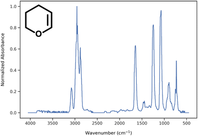
During data preprocessing, all IR spectra were normalized and converted to a series of 1800 data points covering the wavenumber range of 450 cm−1 to 4050 cm−1 with an increment of 2 cm−1. An example of preprocessed IR spectra is shown in Fig. 1. All units in the x-axis and y-axis were converted to wavenumbers and absorbance values, respectively. The absorbance values on each spectrum were linearly normalized to range from 0 to 1 using the following equation: | (1) |
2.3 Neural network models
All untrained neural network models (GCN, GAT, MPNN, AttentiveFP, DNN) were imported from the DeepChem library35 and trained as described below. Each model takes the structural data saved as molecular graph objects or MorganFP descriptors and the preprocessed spectral data as inputs. The RDKit library36 was used to convert the structural data into SMILES and then to MorganFP. The DeepChem library35 was used to convert the SMILES into molecular graph objects.2.4 Training
Each model was trained using a batch size of 64 substances for 100 epochs. The hyperparameters were optimized using Gaussian process hyperparameter optimization. In order to fully leverage the limited amount of data on hand, 5-fold cross validation was used. In case there are multiple spectra for a single compound, all entries for the same compound are placed into the same fold. For each iteration of training and testing, 4 folds were used to train a model and 1 fold was used to test the performance. Euclidean distances between the predicted and actual spectra of each compound were used as the loss function for the training of each model.2.5 Evaluation of prediction performance
For evaluation, predicted and actual spectra were smoothed over by applying a Gaussian Convolution function with a standard deviation of 6 cm−1 using the SciPy library38 in order to remove noise in low absorbance regions in the spectra. The mean of Spearman and Pearson correlation coefficients between predicted and actual spectra were then calculated and used as the metric to evaluate the performance of the trained models.2.6 Comparison of different models
To compare the behavior of the trained models, we calculated Spearman and Pearson correlation coefficients between spectra that were generated by different models for each respective compound. The average values of these correlation coefficients were used to gain insights on the similarity between each pair of models.3 Results and discussion
3.1 Performance of ML models
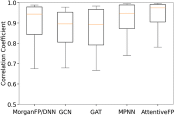
Table 3 summarizes the performance of each model based on Spearman and Pearson correlation coefficients between predicted and actual spectra. GCN, the baseline graph convolutional network model, and GAT, a variant of GCN with the attention mechanism, showed reasonably good yet the lowest performances. It should be noted that these two models showed lower performances in comparison to MorganFP/DNN, the benchmark molecular descriptor-based model. On the other hand, MPNN and AttentiveFP, which utilize the message passing mechanism, showed superior performances in comparison to GCN and GAT. This result indicates that the propagation of node information to neighboring atoms through the message passing mechanism led to an improved performance. Among all tested models, AttentiveFP showed the best performance with the mean Spearman and Pearson correlation coefficient values of 0.911 and 0.925, respectively. As shown in Fig. 2, a closer look of the data indicated that AttentiveFP outperforms MPNN and MorganFP/DNN when we compare the values at each displayed percentile (10th, 25th, 50th, 75th, and 90th) of Spearman correlation coefficients. In particular, the 10th percentile value for AttentiveFP was higher by 4.0% and 10.6% over MPNN and MorganFP/DNN, respectively. This implies that the application of the graph attention mechanism along with the message passing mechanism allows for the network to generate fewer poor predictions while improving the prediction accuracy for most spectra. We attributed this to the advantage of AttentiveFP that is capable of effectively learning some of the important interactions between distant atoms.| Model name | Spearman | Pearson |
|---|---|---|
| MorganFP/DNN | 0.899 | 0.863 |
| GCN | 0.847 | 0.855 |
| GAT | 0.851 | 0.855 |
| MPNN | 0.890 | 0.910 |
| AttentiveFP | 0.911 | 0.925 |
To compare the similarity of the different models, we calculated the mean Spearman correlation coefficients between the IR spectra predicted by each pair of models (Fig. 3). As it can be seen, the IR spectra predicted by GAT shared the highest similarity with GCN whereas they were less similar to MPNN and AttentiveFP. On the other hand, the spectra predicted by MPNN and AttentiveFP are similar to each other. This implies that the propagation of node information by the message passing mechanism substantially affects the behavior of the models. It was also found that the MorganFP/DNN behaves more similarly to MPNN and AttentiveFP than GCN and GAT. A plausible interpretation for this is that MorganFP/DNN is capable of learning interactions between both neighboring and distant atoms as long as they are within the predetermined radius, making the model more similar to MPNN and AttentiveFP.
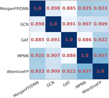 | ||
| Fig. 3 The heatmap of the mean Spearman correlation coefficients of the spectra predicted by different model pairs for identical compounds. | ||
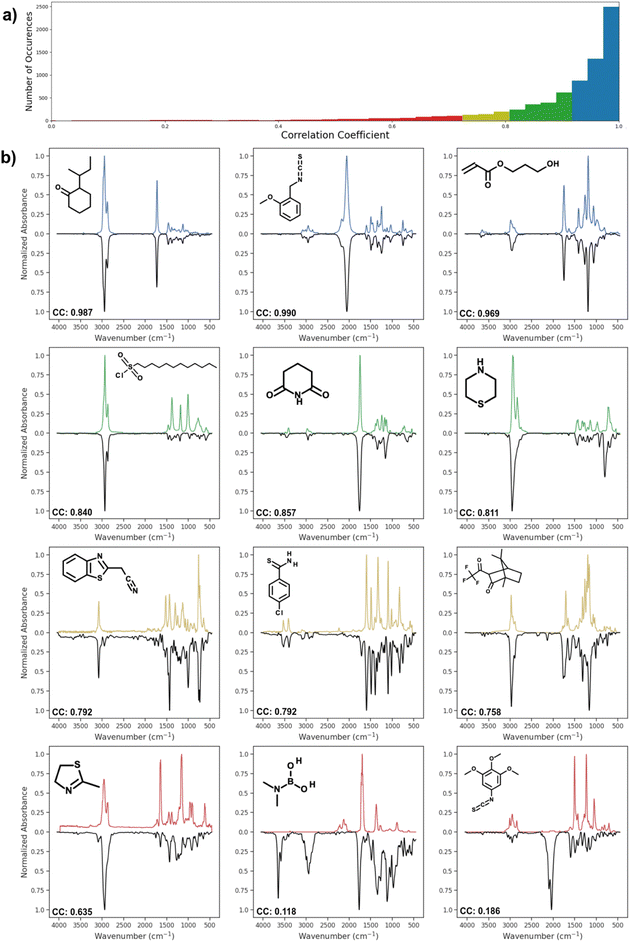
Fig. 4 shows the distribution of correlation coefficient values between actual spectra and spectra predicted by AttentiveFP model, which showed the highest performance. The correlation coefficients of the predicted and actual spectra are 0.9 or higher in approximately 76% of the predicted spectra. As it can be seen, these predicted spectra exhibited high similarity to their corresponding actual spectra. Approximately 12% of the predicted spectra showed moderately high correlation coefficients, 0.80–0.90. In those cases, the location of peaks are often correctly predicted while there appeared to be a tendency of the relative peak intensities being less accurately predicted. Approximately 12% of the predicted spectra had correlation coefficients below 0.8. However, it is worth noting that these comparatively less accurate spectra still often contain some of the major features of actual spectra. In a limited number of cases, as can be seen in the spectrum shown on the bottom right of Fig. 4, the predicted spectra contain large additional peaks or miss major peaks. We carried out several attempts of exploratory data analyses in order to determine if there are any trends among these poorly predicted cases. However, no clear patterns could be observed.
3.2 Factors that affect the IR spectra prediction performance of AttentiveFP model
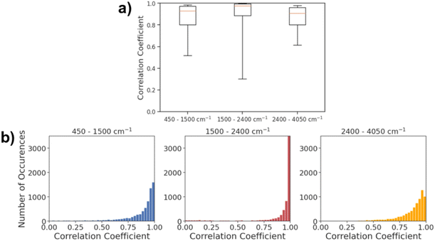
Fig. 5a shows the histogram of correlation coefficients between actual IR spectra and the spectra predicted by AttentiveFP model in three different spectral regions. The characteristic peaks that appear in each of these regions are: O–H, N–H, and C–H stretching (2400–4000 cm−1), C![[double bond, length as m-dash]](https://www.rsc.org/images/entities/char_e001.gif) O, C
O, C![[double bond, length as m-dash]](https://www.rsc.org/images/entities/char_e001.gif) N, and C
N, and C![[double bond, length as m-dash]](https://www.rsc.org/images/entities/char_e001.gif) C stretching, and N–H bending (1500 and 2400 cm−1). As shown in Fig. 5b, the average Spearman correlation coefficient was highest in the 2400–4050 cm−1 region followed by 1500–2400 cm−1 region. In all three regions, the peak of each histogram was observed in either the highest bin (above 0.96) or the second highest bin (0.93–0.96). The 50th percentile values of the correlation coefficients are 0.929, 0.977, and 0.909, for the 450–1500, 1500–2400 and 2400–4050 cm−1 ranges, respectively. This indicates that the model was capable of predicting the spectra across the entire mid-IR range in majority of the cases. On the other hand, the 10th percentile value of the correlation coefficient for the 1500–2400 cm−1 region was 0.300. This value is substantially lower than 0.519 and 0.614, respectively, for 450–1500 and 2400–4050 cm−1 regions. This is reflected in Fig. 5b, as the gap between 25th percentile and 10th percentile is substantially larger in the 1500–2400 cm−1 region when compared to the 450–1500 and 2400–4050 cm−1 regions. The result indicates that the model predicts the spectra within 1500–2400 cm−1 regions with high accuracy in more than 75% of the cases while there are a relatively small number of cases where the predicted spectra poorly resemble actual spectra. In terms of the mean Spearman correlation coefficient values, the performance of the model was comparatively lower in the 450–1500 cm−1 region than other spectral regions. This is unsurprising since this spectral region is called the ‘fingerprint’ region where it is known to be highly complex due to the presence of many bands that frequently overlap with each other. This is also in line with results from past attempts at spectral prediction using machine learning, where the fingerprint region typically has the worst results.21
C stretching, and N–H bending (1500 and 2400 cm−1). As shown in Fig. 5b, the average Spearman correlation coefficient was highest in the 2400–4050 cm−1 region followed by 1500–2400 cm−1 region. In all three regions, the peak of each histogram was observed in either the highest bin (above 0.96) or the second highest bin (0.93–0.96). The 50th percentile values of the correlation coefficients are 0.929, 0.977, and 0.909, for the 450–1500, 1500–2400 and 2400–4050 cm−1 ranges, respectively. This indicates that the model was capable of predicting the spectra across the entire mid-IR range in majority of the cases. On the other hand, the 10th percentile value of the correlation coefficient for the 1500–2400 cm−1 region was 0.300. This value is substantially lower than 0.519 and 0.614, respectively, for 450–1500 and 2400–4050 cm−1 regions. This is reflected in Fig. 5b, as the gap between 25th percentile and 10th percentile is substantially larger in the 1500–2400 cm−1 region when compared to the 450–1500 and 2400–4050 cm−1 regions. The result indicates that the model predicts the spectra within 1500–2400 cm−1 regions with high accuracy in more than 75% of the cases while there are a relatively small number of cases where the predicted spectra poorly resemble actual spectra. In terms of the mean Spearman correlation coefficient values, the performance of the model was comparatively lower in the 450–1500 cm−1 region than other spectral regions. This is unsurprising since this spectral region is called the ‘fingerprint’ region where it is known to be highly complex due to the presence of many bands that frequently overlap with each other. This is also in line with results from past attempts at spectral prediction using machine learning, where the fingerprint region typically has the worst results.21
Finally, we investigated whether the performance of AttentiveFP model would be affected by the number of non-hydrogen atoms that are present in the compounds (Fig. 6). Interestingly, the result indicated that the performances of AttentiveFP model are not affected by the number of non-hydrogen atoms for the compounds consisting of 5 to 24 non-hydrogen atoms. Meanwhile, the comparatively lower prediction performance for the compounds consisting of 2–4 non-hydrogen atoms. Although the reasons are unclear, possible causes for this could be due to the low occurrences of these classes of molecules within the dataset (Fig. S1 in ESI†) and a higher frequency of halogenated compounds.
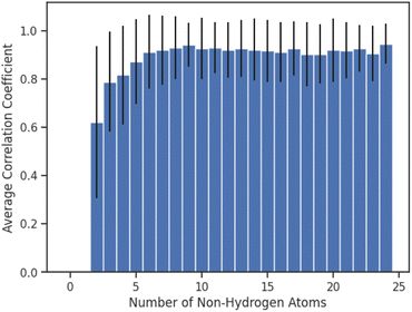 | ||
| Fig. 6 Average of Spearman correlation coefficient values for compounds consisting of different numbers of non-hydrogen atoms. Error bars correspond to the standard deviation. | ||
3.3 Interpretation of attention weights
At its core, attention allows neural networks to dynamically prioritize specific segments of the input data when generating output, mimicking human cognitive processes of selective concentration. Traditional sequence-to-sequence models encode inputs into fixed-size vectors, but attention facilitates a more adaptive approach. In the AttentiveFP model, an attention vector is calculated by assessing the relevance for each input–output pair, applying a softmax function, and creating a context vector from a weighted sum in order to emphasize the effects of certain molecular features that have a greater impact on the spectrum.30We therefore looked into the attention values being assigned by the AttentiveFP model (Table S3†). In this respect we first compared the average attention values on the atoms within pairs of structurally similar functional groups. The average attention values on the two non-hydrogen atoms in alcohols (O and adjacent C) weigh above the baseline attention values. On the other hand, atoms in thiols and alkyl halides show comparatively lower attention values which are closer to the baseline. The average attention values on the atoms on carboxylic acids are higher than the atoms on acyl halides. In the case of the AttentiveFP model reported by Xiong et al.30 higher attention values were assigned on the atoms in aromatic systems when the model was trained to predict the number of aromatic atoms. The comparison of attention values on different classes of carbon atoms provided insights on how the attention mechanism could capture the influences of distant atoms. In contrast, our IR-spectra prediction models showed a tendency to assign higher attention values to non-aromatic carbons in alkyl chains and alkene over carbons in aromatic systems. Considering the fact that all carbon–hydrogen bonds and carbon–carbon bonds manifest different peaks on IR spectra, the observed deviations among different classes of carbon atoms are reasonable. We also confirmed that the attention values are not biased toward the more abundant functional groups (Fig. S4†). These observations collectively support that the attention mechanism allowed for the AttentiveFP model to learn the impact of adjacent and distant atoms for the IR spectra prediction task.
4 Conclusions
In this work, we have studied the performance of graph neural networks for the prediction of the IR spectra. Our results showed that AttentiveFP model outperformed other graph neural network models as well as MorganFP/DNN model, the benchmark descriptor-based model. Approximately 88% of the spectra generated by AttentiveFP model showed high similarity, with the correlation coefficients being 0.80 or above, to experimentally determined spectra. An interesting observation was that the average correlation coefficient values between the spectra predicted by AttentiveFP model and actual spectra for molecules consisting of 12 or more non-hydrogen atoms are similar to comparatively smaller molecules consisting of 5–11 non-hydrogen atoms. In summary, our results demonstrate that the implementation of the attention mechanism is an effective approach to improve the performance of graph neural networks in mapping IR spectra from chemical structures.Code availability
The codes for this paper are available at GitHub at https://github.com/nj-saquer/IR-Spectra-Prediction-Graph-Models/.Data availability
This study was carried out using publicly available data on IR spectra from the NIST Chemistry WebBook database at https://doi.org/10.18434/T4D303. The codes that were used to retrieve and preprocess the datasets are available at GitHub along with other code.Author contributions
N. S. conceptualization, data curation, formal analysis, investigation, methodology, validation, software, visualization, writing – original draft, writing – review & editing; R. I. conceptualization, methodology, funding acquisition, investigation, project administration, supervision, writing – review & editing; J. D. E. conceptualization, data curation, methodology; K. Y. conceptualization, methodology, funding acquisition, investigation, project administration, supervision, writing – original draft, writing – review & editing.Conflicts of interest
There are no conflicts to declare.Acknowledgements
This work was supported by the NASA-Missouri Space Grant Consortium (NASA-MOSGC). N. S. was partly supported by the NASA-MOSGC undergraduate research internship program. We also acknowledge NIST for making the IR spectra data available.Notes and references
- C. Berthomieu and R. Hienerwadel, Photosynth. Res., 2009, 101, 157–170 CrossRef CAS PubMed.
- J. Haas and B. Mizaikoff, Annu. Rev. Anal. Chem., 2016, 9, 45–68 CrossRef PubMed.
- T. Theophanides, Infrared Spectroscopy: Materials Science, Engineering and Technology, IntechOpen, London, 2012 Search PubMed.
- M. R. Jung, F. D. Horgen, S. V. Orski, V. Rodriguez C, K. L. Beers, G. H. Balazs, T. T. Jones, T. M. Work, K. C. Brignac and S.-J. Royer, et al. , Mar. Pollut. Bull., 2018, 127, 704–716 CrossRef CAS PubMed.
- M. J. Baker, J. Trevisan, P. Bassan, R. Bhargava, H. J. Butler, K. M. Dorling, P. R. Fielden, S. W. Fogarty, N. J. Fullwood and K. A. Heys, et al. , Nat. Protoc., 2014, 9, 1771–1791 CrossRef CAS PubMed.
- K. B. Beć, J. Grabska and C. W. Huck, Anal. Chim. Acta, 2020, 1133, 150–177 CrossRef PubMed.
- T. P. Wrobel and R. Bhargava, Anal. Chem., 2017, 90, 1444–1463 CrossRef PubMed.
- K. D. Shepherd and M. G. Walsh, J. Near Infrared Spectrosc., 2007, 15, 1–19 CrossRef CAS.
- G. Tinetti, T. Encrenaz and A. Coustenis, Astron. Astrophys. Rev., 2013, 21, 1–65 CrossRef.
- G. H. Rieke, Exp. Astron., 2009, 25, 125–141 CrossRef.
- M. Thomas, M. Brehm, R. Fligg, P. Vöhringer and B. Kirchner, Phys. Chem. Chem. Phys., 2013, 15, 6608 RSC.
- J. Vamathevan, D. Clark, P. Czodrowski, I. Dunham, E. Ferran, G. Lee, B. Li, A. Madabhushi, P. Shah and M. Spitzer, et al. , Nat. Rev. Drug Discovery, 2019, 18, 463–477 CrossRef CAS PubMed.
- A. C. Mater and M. L. Coote, J. Chem. Inf. Model., 2019, 59, 2545–2559 CrossRef CAS PubMed.
- D. C. Elton, Z. Boukouvalas, M. D. Fuge and P. W. Chung, Mol. Syst. Des. Eng., 2019, 4, 828–849 RSC.
- X. Yang, Y. Wang, R. Byrne, G. Schneider and S. Yang, Chem. Rev., 2019, 119, 10520–10594 CrossRef CAS PubMed.
- M. Gastegger, J. Behler and P. Marquetand, Chem. Sci., 2017, 8, 6924–6935 RSC.
- M. Gastegger, K. T. Schütt and K.-R. Müller, Chem. Sci., 2021, 12, 11473–11483 RSC.
- J. Lam, S. Abdul-Al and A.-R. Allouche, J. Chem. Theory Comput., 2020, 16, 1681–1689 CrossRef CAS PubMed.
- G. Laurens, M. Rabary, J. Lam, D. Peláez and A.-R. Allouche, Theor. Chem. Acc., 2021, 140, 66 Search PubMed.
- C. Affolter and J. Clerc, Chemom. Intell. Lab. Syst., 1993, 21, 151–157 CrossRef CAS.
- U. Weigel and R. Herges, Anal. Chim. Acta, 1996, 331, 63–74 CrossRef CAS.
- P. Kovács, X. Zhu, J. Carrete, G. K. Madsen and Z. Wang, Astrophys. J., 2020, 902, 100 CrossRef.
- C. McGill, M. Forsuelo, Y. Guan and W. H. Green, J. Chem. Inf. Model., 2021, 61, 2594–2609 CrossRef CAS PubMed.
- O. Wieder, S. Kohlbacher, M. Kuenemann, A. Garon, P. Ducrot, T. Seidel and T. Langer, Drug Discovery Today: Technol., 2020, 37, 1–12 CrossRef PubMed.
- D. Rogers and M. Hahn, J. Chem. Inf. Model., 2010, 50, 742–754 CrossRef CAS PubMed.
- R. Todeschini and V. Consonni, Molecular Descriptors for Chemoinformatics, Wiley, Weinheim, 2009 Search PubMed.
- C. Merkwirth and T. Lengauer, J. Chem. Inf. Model., 2005, 45, 1159–1168 CrossRef CAS PubMed.
- D. K. Duvenaud, D. Maclaurin, J. Iparraguirre, R. Bombarell, T. Hirzel, A. Aspuru-Guzik and R. P. Adams, Advances in Neural Information Processing Systems 28 (NIPS 2015), 2015 Search PubMed.
- S. Kearnes, K. McCloskey, M. Berndl, V. Pande and P. Riley, J. Comput.-Aided Mol. Des., 2016, 30, 595–608 CrossRef CAS PubMed.
- Z. Xiong, D. Wang, X. Liu, F. Zhong, X. Wan, X. Li, Z. Li, X. Luo, K. Chen and H. Jiang, et al. , J. Med. Chem., 2019, 63, 8749–8760 CrossRef PubMed.
- P. Veličković, G. Cucurull, A. Casanova, A. Romero, P. Liò and Y. Bengio, Graph Attention Networks, 2017, https://arxiv.org/abs/1710.10903 Search PubMed.
- D. Jiang, Z. Wu, C.-Y. Hsieh, G. Chen, B. Liao, Z. Wang, C. Shen, D. Cao, J. Wu and T. Hou, J. Cheminf., 2021, 13, 1–23 Search PubMed.
- Coblentz Society Inc., Evaluated Infrared Reference Spectra, in NIST Chemistry WebBook, NIST Standard Reference Database Number 69, ed. P. J. Lindstrom and W. G. Mallard, National Institute of Standards and Testing, Gaithersburg MD, accessed January, 2022, DOI:10.18434/T4D303.
- M. Swaine, nist.py, 2015, https://gist.github.com/mcs07/48fcfc0f072e5f45dcaa, accessed January, 2022 Search PubMed.
- B. Ramsundar, P. Eastman, P. Walters and V. Pande, Deep learning for the life sciences: applying deep learning to genomics, microscopy, drug discovery, and more, O'Reilly, Sebastopol, 2019 Search PubMed.
- G. Landrum, RDKIT: open-source cheminformatics software, https://rdkit.org/ Search PubMed.
- J. Gilmer, S. S. Schoenholz, P. F. Riley, O. Vinyals and G. E. Dahl, Proceedings of the 34th International Conference on Machine Learning, PMLR 70, 2017, pp. 1263–1272 Search PubMed.
- P. Virtanen, R. Gommers, T. E. Oliphant, M. Haberland, T. Reddy, D. Cournapeau, E. Burovski, P. Peterson, W. Weckesser, J. Bright, S. J. van der Walt, M. Brett, J. Wilson, K. J. Millman, N. Mayorov, A. R. J. Nelson, E. Jones, R. Kern, E. Larson, C. J. Carey, İ. Polat, Y. Feng, E. W. Moore, J. VanderPlas, D. Laxalde, J. Perktold, R. Cimrman, I. Henriksen, E. A. Quintero, C. R. Harris, A. M. Archibald, A. H. Ribeiro, F. Pedregosa, P. van Mulbregt and SciPy 1.0 Contributors, Nat. Methods, 2020, 17, 261–272 CrossRef CAS PubMed.
Footnote |
| † Electronic supplementary information (ESI) available: Supporting tables and figures on the composition of dataset, histogram of correlation coefficient values for all tested models, and attention values. See DOI: https://doi.org/10.1039/d3dd00254c |
| This journal is © The Royal Society of Chemistry 2024 |

