
 Open Access Article
 This Open Access Article is licensed under a
 Creative Commons Attribution 3.0 Unported Licence
Race to the bottom: Bayesian optimisation for chemical problems†
Yifan
Wu
a,
Aron
Walsh
 *ab and
Alex M.
Ganose
*c
*ab and
Alex M.
Ganose
*c
aDepartment of Materials, Imperial College London, London SW7 2AZ, UK. E-mail: a.walsh@imperial.ac.uk
bDepartment of Physics, Ewha Womans University, Seoul 03760, Korea
cDepartment of Chemistry, Molecular Sciences Research Hub, White City Campus, Imperial College London, Wood Lane, London W12 0BZ, UK. E-mail: a.ganose@imperial.ac.uk
First published on 20th May 2024
Abstract
What is the minimum number of experiments, or calculations, required to find an optimal solution? Relevant chemical problems range from identifying a compound with target functionality within a given phase space to controlling materials synthesis and device fabrication conditions. A common feature in this application domain is that both the dimensionality of the problems and the cost of evaluations are high. The selection of an appropriate optimisation technique is key, with standard choices including iterative (e.g. steepest descent) and heuristic (e.g. simulated annealing) approaches, which are complemented by a new generation of statistical machine learning methods. We introduce Bayesian optimisation and highlight recent success cases in materials research. The challenges of using machine learning with automated research workflows that produce small and noisy data sets are discussed. Finally, we outline opportunities for developments in multi-objective and parallel algorithms for robust and efficient search strategies.
Introduction
With the development of automation technologies, combinatorial and high-throughput chemical synthesis is increasingly applied to discover new materials and molecules.1–3 Enumerating over large chemical spaces becomes impractical as the number of synthesis parameters increases—termed “the curse of high dimensionality”—and is difficult to justify with the push towards more sustainable and efficient research practices.4 Smart automation techniques, such as algorithms to suggest which experiments to perform next, can accelerate the materials discovery process and dramatically increase the cost-effectiveness of research.5,6 Such techniques cover the full synthesis pipeline, from identifying target chemical spaces with desired properties using ab initio or machine-learned property predictions, to suggesting synthesis routes with digital retrosynthesis and chemical reaction prediction through to synthesising and characterising candidates with fully autonomous robotics platforms.7 Data-driven algorithms for experiment selection can be used to minimise the overall cost of chemical discovery, in terms of the number of experiments performed, time spent, or use of materials. This process can be framed as an optimisation problem.Optimisation is critical to any problem involving decision-making8 and is the process of systematically choosing input parameters (experimental conditions, precursors, etc.) to minimise or maximise an objective function (e.g., running an experiment and performing a measurement). The objective function can be arbitrarily defined and is typically derived from a specific property of the system under study. The process of optimisation can be summarised as
 | (1) |
 | (2) |
 is the domain of interest. When considering complex high-dimensional landscapes, there are often many minima (stationary points of the target function or experiment) which make finding the global minimum exceedingly difficult (Fig. 1). This process is termed global optimisation. Examples include hyperparameter optimisation of supervised machine learning algorithms (in this case, the objective function may be the mean average error [MAE] or mean squared error [MSE] of the model),9 solving the geometric structure of proteins and crystal structures (here the objective function is the root mean squared error in the atomic positions),10 and choosing the architecture and synthesis conditions for functional devices (where the objective function is the figure of merit of the device).
 | ||
| Fig. 1 Illustration of optimisation in surfaces with increasing complexity and number of dimensions. | ||
To find the minimum or maximum of a function, f, the first intuition for a mathematician is to differentiate the function and let its derivative equal zero. Numerically, this can be achieved by gradient descent, which is an iterative approach to minimise a differentiable objective function by moving towards the direction of steepest descent.11 Mathematically, this can be written
| xn+1 = xn + γ∇f(xn), | (3) |
The field of optimisation has seen a renaissance with the development of accurate machine learning models. Machine learning is a statistical method that relies on the relationships between input parameters and target outputs, and can be applied to model, optimise, and evaluate a target system.17,18 The integration of machine learning and optimisation has led to a new class of optimisation algorithms termed Bayesian optimisation. The Bayesian method is an active learning approach that applies a sequential strategy to solve optimisation problems19 and has been used to find the optima of complex functions in chemistry, biology, and materials science.20 A summary of different optimisation methods and their associated hyperparameters is summarised in Table 1.
| Algorithm | Key hyperparameter | Functional space |
|---|---|---|
| Gradient descent | Step size γ | Continuous and convex |
| Simulated annealing | Accept rate r | Discrete and multi-optima |
| Bayesian optimisation | Exploitation and exploration rate λ | Discrete and unknown |
In this work, we outline the principles of Bayesian optimisation, including the mathematical foundation and choice of surrogate and acquisition functions. We examine how optimisation has been implemented in the chemical sciences, particularly focusing on automated research workflows. We discuss state-of-the-art approaches for handling small, noisy, or high-dimensional datasets. Finally, we outline the opportunities for developments in hybrid algorithms for robust and efficient searches.
Bayesian optimisation
At the heart of Bayesian optimisation is Bayes' theorem, named after Thomas Bayes (1701–1761). While Bayes never published his most famous accomplishment, his notes were collected and published posthumously by Richard Price in 1763.21 Bayes' theorem describes the correlation between two different events and is used to calculate the conditional probability of one event happening based on the condition that another event has occurred.22 If A and B are two events, the probability of A happening given the conditional event B is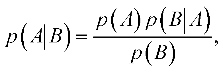 | (4) |
The term Bayesian optimisation is attributed to Jonas Mockus from his work on global optimisation during the 1970s and 1980s.24,25 Bayesian optimisation uses a sequential model-based strategy for global optimisation. There are two key concepts: (i) a surrogate function (statistical model) is introduced to estimate the posterior distribution of the objective function;26,27 and (ii) an acquisition function is used to evaluate the domain of inputs and determine which point to sample next.
The Bayesian optimisation cycle starts with the known points of the objective function. The surrogate model is used to estimate the remaining distribution of the objective function (termed the posterior predictive distribution or just the posterior). The mean and variance of the posterior are fed into the acquisition function and the point with the maximum value selected. This becomes the new observation point and the objective function is evaluated—in chemical problems, this amounts to performing an experiment and measuring a property. After each iteration, the new sample point is added to the set of observations, the posterior predictive distribution is reevaluated using the surrogate model, the mean and variance are recalculated, and the acquisition function is used to select the next input point. This process is repeated until the maximum number of learning cycles (or another convergence criterion) is reached (Fig. 2). Bayesian optimisation has the advantage that it can be applied to complex search spaces with multiple categorical or conditional inputs. Several software libraries have been developed for performing Bayesian optimisation (Table 2) and packages to increase its accessability for real-world tasks such as Honegumi.28
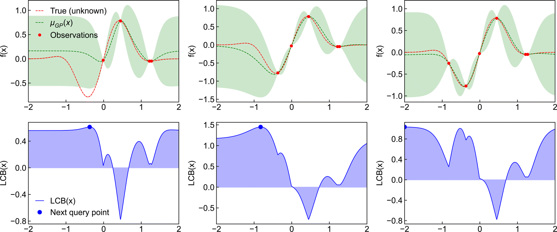 | ||
| Fig. 2 Demonstration of the Bayesian optimisation procedure for a 1D function. Top left panel: the true objective function (red dashed line) is approximated by a Gaussian process (green dashed line) based on several experimental observations (red circles) with the uncertainty shown by the green shaded region. Bottom left panel: the acquisition function (blue solid line) across the function domain, with the next query point highlighted (blue circle). The middle and right panels display the same information with additional experimental observations included. | ||
| Package | Models | Features | License | Ref. |
|---|---|---|---|---|
| a https://ax.dev. b https://github.com/zavalab/bayesianopt. c https://github.com/fmfn/BayesianOptimization. d https://botorch.org. e https://github.com/tsudalab/combo. f https://github.com/dragonfly/dragonfly. g https://sheffieldml.github.io/GPyOpt. h http://hyperopt.github.io/hyperopt. i https://nextorch.readthedocs.io. j https://optuna.readthedocs.io. k https://scikit-optimize.github.io. l https://automl.github.io/SMAC3/main/. m https://github.com/ziatdinovmax/gpax. n https://matter-atlas.readthedocs.io. o https://cest-group.gitlab.io/boss. p https://github.com/b-shields/edbo. q https://github.com/leojklarner/gauche. r https://github.com/mikediessner/nubo. s https://github.com/aspuru-guzik-group/olympus. t https://github.com/aspuru-guzik-group/phoenics. u https://gosummit.readthedocs.io. | ||||
| General purpose | ||||
| Axa | GP, others | Modular framework built on BoTorch | MIT | |
| Bayesianoptb | GP | Parallel optimisation | MIT | 29 |
| BayesOptc | GP | Single objective | MIT | 30 |
| BoTorchd | GP, others | Multi-objective optimisation | MIT | 31 |
| COMBOe | GP | Multi-objective optimisation | MIT | 32 |
| Dragonflyf | GP | Multi-fidelity optimisation | Apache | 33 |
| GPyOptg | GP | Parallel optimisation | BSD | 34 |
| Hyperopth | TPE | Serial/parallel optimisation | BSD | 35 |
| NEXTorchi | GP, others | Modular framework built on BoTorch | MT | 36 |
| Optunaj | RF | Hyperparameter tuning | MIT | 37 |
| Skoptk | RF, GP | Batch optimisation | BSD | 38 |
| SMAC3l | GP, RF | Hyperparameter tuning | BSD | 39 |
| GPaxm | GP | Multi-task/fidelity | MIT | 40 and 41 |
![[thin space (1/6-em)]](https://www.rsc.org/images/entities/char_2009.gif) |
||||
| Physical science domain | ||||
| Atlasn | GP | Mixed-parameter optimisation for self-driving labs | MIT | 42 |
| BOSSo | GP | Crystal structure optimisation | Apache | 43 |
| Edbop | GP | Tailored chemical synthesis descriptors | MIT | 5 |
| GAUCHEq | GP | Tailored molecular representations | MIT | 44 |
| NUBOr | GP | Transparent BO to personalise problem | BSD | 45 |
| Olympuss | GP, TPE, BNN | Benchmarking and noisy optimisation | MIT | 46 |
| Phoenicst | BNN | Bayesian kernel density estimation | Apache | 47 |
| Summitu | GP, RF | Multi-task optimisation for chemical reactions | MIT | 48 |
Surrogate models
Surrogate models are used to estimate the value and uncertainty in the unseen portion of the objective function. Consider the situation where there are two initial known points on a 1D optimisation surface. We can guess the path that the objective function takes between the two points. By making many such guesses, we will build up a distribution of paths. The distribution will be narrower in the regions around the two known points and broadest roughly halfway between the points. This distribution of target values is similar to known probability distributions, such as a Gaussian process. Since we can now estimate the distribution of the target property, we can calculate the mean and variance across the domain and use it in the acquisition function. We now provide a summary of the two most common surrogate models.Gaussian processes
Gaussian processes are a class of stochastic regression model and are widely employed in Bayesian optimisation.49 The key concept of Gaussian processes is to model the objective function as a multivariate normal distribution. A Gaussian process on f with a set of input points X = {x1, x2, x3, …, xn} is specified by a mean function μ and covariance function or kernel Σ as | (5) |
The mean function determines the expected function value at any location x. The kernel determines the shape of the distribution at each location and the properties of the function's behaviour. The kernel takes two locations x, x′ as inputs and returns a scalar similarity measure between those two points as output
| ΣXX = Cov(x, x′). | (6) |
Several kernels are available that confer a range of properties such as smoothness or periodicity, such as the radial basis function kernel.
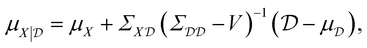
The starting point for Gaussian process regression is a multivariate normal distribution defined over the objective function. In the case of no observed training data, this is termed the prior distribution, pX. Typically it is assumed μX = 0 for simplicity and the kernel function is chosen based on an initial guess of the properties of the objective function. Given a set of observations,  , we can “condition” the prior to produce a new distribution (which is also Gaussian), termed the posterior distribution
  by forming the joint distribution.
 | (7) |
The conditioned mean and covariance functions are defined by
 | (8) |
 | (9) |
One can now extract the mean and standard deviation of the posterior distribution at each location for use by the acquisition function.
Random forest
Random forest is a supervised machine learning algorithm utilising an ensemble of decision trees.50,51 A decision tree is an approach to predict the target value of a data point through a series of binary choices based on the input features.52 For classification tasks, the final output of a random forest is the class selected by the most trees. For regression tasks, the final output is the average prediction across all trees. By combining multiple decision trees, random forests correct for overfitting to the training set.53 Random forests utilise an ensemble of B decision trees, {Tb}B1, each trained on a different and randomly selected subset of the input features, Xb. In regression tasks, the mean and variance of random forests is given by | (10) |
 | (11) |
Compared with Gaussian processes,54 random forests can extend more easily to higher dimensional problems.55 Furthermore, the evaluation time for Gaussian processes scales cubically with the number of training samples. While various sparse techniques have been developed to reduce computation time, Gaussian processes are generally limited to problems with less than a few thousand data points (n) due to the necessary covariance matrix inversion with a computational complexity of O(n3). However, in experimental materials science and chemistry domains with relatively small dataset sizes, Gaussian processes are often the surrogate model of choice for Bayesian optimisation due to their relatively small number of hyperparameters and high out-of-the-box accuracy.
Acquisition functions
Acquisition functions use the mean μ and variance σ computed from surrogate models to decide which point to search next. The process of choosing the next point has three main considerations: (i) exploitation (i.e., maximisation or minimisation) of the objective function; (ii) exploration of unknown regions of parameter space; and (iii) the risk or uncertainty of predictions. Different acquisition functions have been developed to balance these considerations, including the “expected improvement” (EI), “probability of improvement” (PI) and “lower confidence bound” (LCB) approaches. Below, we outline these methods and their typical applications.Probability of improvement
The first activation function designed for Bayesian optimisation was probability of improvement. If f′ is the maximum value of the objective function observed so far, we can define improvement, I, as| I(x) = max(f(x) − f′, 0). | (12) |
Accordingly, the improvement will only be positive if the new point has a value greater than f′. In probability of improvement, we evaluate the point most likely to improve upon this value using the following utility function
 | (13) |
Thus, we receive a reward if f(x) is greater than f′ and no reward otherwise. The acquisition function is the expectation of the utility function, in other words, the total probability that I(x) > 0, namely
 | (14) |
Expected improvement
PI only considers the probability of improving the current best estimate but it does not take into account the magnitude of the improvement. This can lead to getting stuck in local optima and underexploration of the parameter space. An alternative acquisition function that accounts for the magnitude of the improvement is expected improvement. Expected improvement is the expectation value of I(x), obtained as | (15) |
 is the probability density function of the normal distribution. Expected improvement selects for values where μ > f′ and for points with high uncertainty. Typical implementations of expected improvement also include a hyperparameter ξ, termed jitter, that tunes the balance between exploitation and exploration by driving the Bayesian optimisation algorithm towards more exploration.
Lower confidence bound
Another simple but powerful acquisition function is lower confidence bound. Here, the acquisition function takes the form| LCB(X) = −λμ + σ | (16) |
Demonstration of optimisation algorithms
We now illustrate the performance of gradient descent, simulated annealing, and Bayesian optimisation in finding the minimum of a relatively simple analytical function (Fig. 3). We have chosen the Sine function, defined by Aldeghi et al.56 as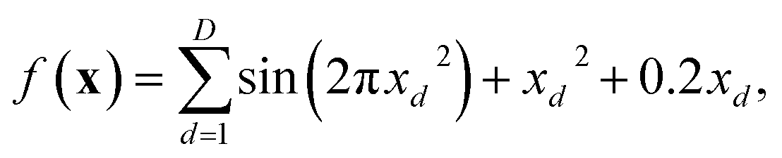 | (17) |
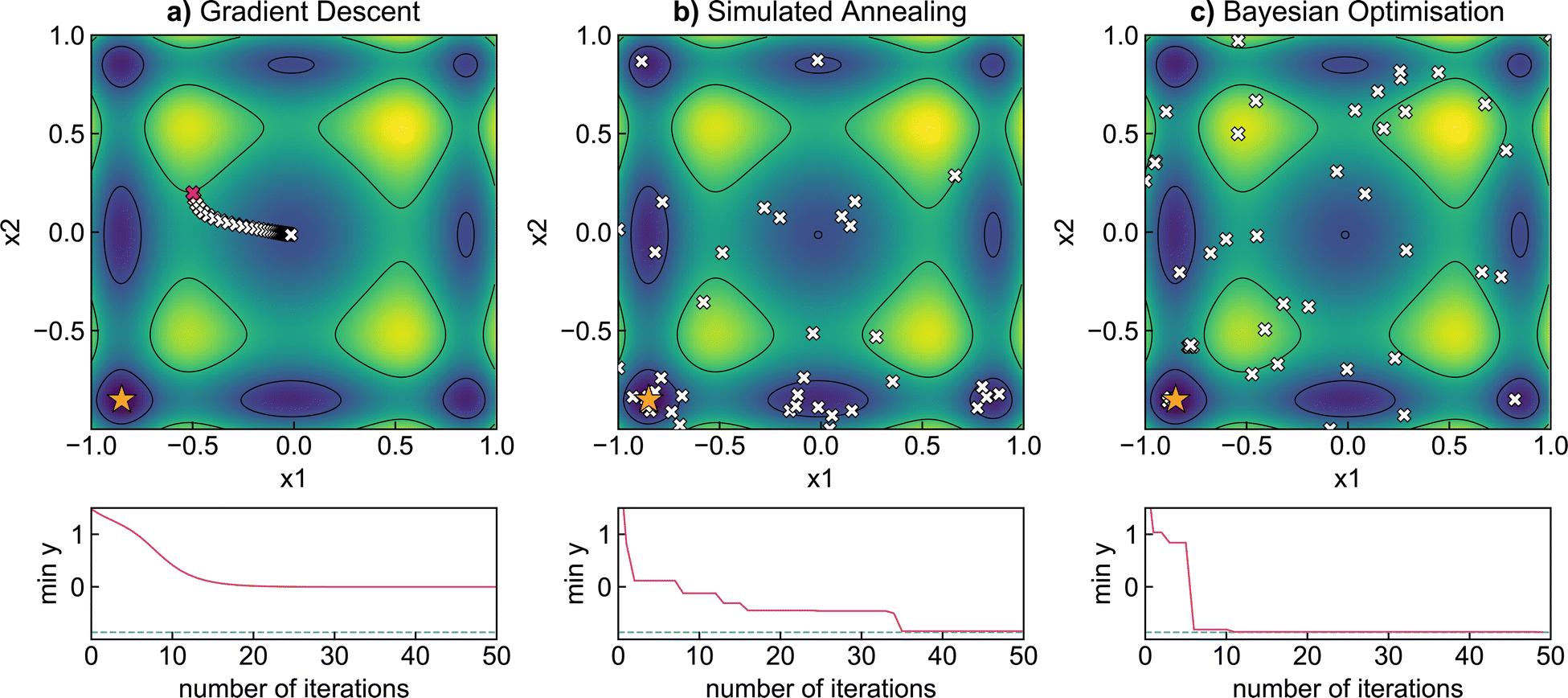 | ||
| Fig. 3 Comparison of optimisation algorithms: (a) gradient descent, (b) simulated annealing, and (c) Bayesian optimisation on the Sine function with 10 minima (see text for details). Typical optimisation trajectories have been displayed in each case. The surfaces illustrate the Sine function, which is not directly observable, but that we would like to optimise. The initial starting point is shown by a red cross, while the true global minimum is indicated with an orange star. Points sampled by the optimisation algorithm are indicated by white crosses. The accompanying subplots illustrate the minimum value observed at each iteration of the optimisation. Bayesian optimisation converges to the true global minimum the quickest while gradient descent fails to find the global minimum. | ||
Photovoltaic device optimisation
For a physical science demonstration, we apply Bayesian optimisation to a photovoltaic device design. The Modelling Solar Cells package57 is used to simulate the power conversion efficiency of a TiO2/ZnO/CdS/Cu2ZnSnS4/Mo solar cell under AM1.5 global sun illumination. This phenomenological approach accounts for radiative, Auger, trap-assisted, and surface recombination losses through shunt resistance. A p-doped Cu2ZnSnS4 absorber layer and n-doped CdS buffer layer form the p–n semiconductor junction. The parameter space controlling the efficiency consists of the thickness and doping concentrations of the absorber and buffer layers, giving rise to a four-dimensional optimisation problem.We evaluate the performance of Bayesian optimisation against a grid search approach that enumerates all potential input parameters on a discretised 4 × 4 × 5 × 5 grid (4 thicknesses and 5 doping concentrations per doping polarity) and random parameter selection over the entire domain (n-type thickness ∈ [10−9, 10−6] m, p-type thickness ∈ [10−8, 10−5] m, and n/p doping concentrations ∈ [1014, 1018] cm−3). Accordingly, even using very coarse sampling of the parameter space, the grid search approach must still sample 400 points for complete coverage. In contrast, it takes less than 20 iterations for Bayesian optimisation to converge to maximum efficiency by effectively using information from early evaluations to focus on promising areas quickly.
The performance of Bayesian optimisation with different acquisition functions against simulated annealing and random sampling is compared in Fig. 4c. Due to the stochastic nature of the optimisation, we repeat the experiment 30 times and plot the standard deviation of predictions in the shaded region. We find Bayesian optimisation converges rapidly to the optimal value of 17.1% in less than 20 iterations, with the expected improvement and upper confidence bound acquisition functions slightly outperforming probability of improvement. Simulated annealing also converges to the optimal value but takes over three times as many iterations. In contrast, random sampling converges much more slowly and only reaches an efficiency of 14.5% after 75 iterations. In Fig. 4a and b we illustrate two-dimensional slices of the optimisation surfaces, highlighting the route Bayesian optimisation samples the parameter space. The optimisation algorithm quickly identifies a p-type thickness of 10−5 m and n-type carrier concentration of 1018 cm−3 as optimal values, and samples the remaining input parameters to find the global maximum. Our results demonstrate the potential of Bayesian optimisation compared to naive grid and random searches.
 | ||
| Fig. 4 Bayesian optimisation outperforms random search in optimising the efficiency of a solar cell. The path taken by the Bayesian optimisation algorithm to identify the global maximum projected on two-dimensional slices of the parameter space, namely (a) p-type CZTS thickness and carrier concentration, and (b) n-type CdS thickness and carrier concentration. The initial point for the optimisation is indicated with a red cross. The optimal input value is identified with a gold star. The points along the optimisation trajectory are indicated in green crosses, varying from light to dark as the number of iterations increases. (c) The performance of Bayesian optimisation with different acquisition functions (Upper Confidence Bound [UCB], Probability of Improvement [PI], Expected Improvement [EI]) against simulated annealing and random search. The optimisation was performed 30 times with the standard deviation of experiments indicated by the shaded regions. | ||
Recent applications to chemical problems
Automated experiments
In the last decade, advances in robotics platforms tailored to the chemical sciences have enabled the rise of automated experiments. These systems can screen large libraries of precursors and experimental conditions more rapidly and reproducibly than human researchers.58 A natural application of Bayesian optimisation is driving the selection of input parameters to minimise or maximise an experimental observable in automated chemical experiments. To understand the performance of Bayesian optimisation on materials science problems, Liang et al.59 compiled five datasets from the literature (Fig. 5) spanning polymeric and nanoparticle formulations, inorganic thin films, and materials manufacturing, with a range of dimensions (3–5) and sample counts (94–600). For each dataset, they evaluated the performance of Bayesian optimisation against random sampling at discovering the percentage of top candidates and the improvement in objective function. Bayesian optimisation using Gaussian processes with anisotropic kernels and a random forest surrogate model was found to outperform random sampling in all cases.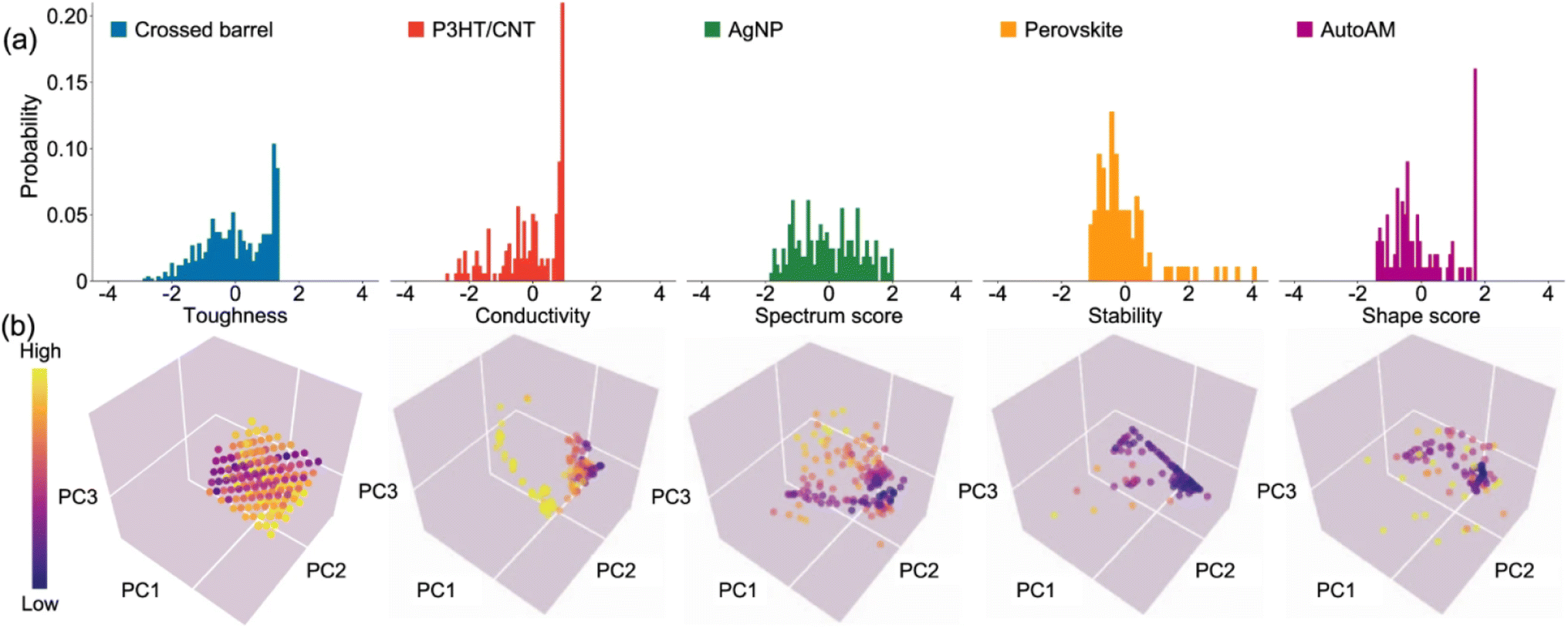 | ||
| Fig. 5 Materials science datasets used to evaluate Bayesian optimisation against random sampling. (a) Histogram of objective values. (b) Input feature space projected onto 3 dimensions using principal component analysis (PCA). Reproduced with permission from Liang et al.59 | ||
Optimisation of chemical reactions is a highly complex, multidimensional problem that requires synthetic chemists to evaluate many parameters, including reagents, concentrations, temperatures, solvents, substrates, and catalysts. Bayesian optimisation has emerged as a powerful tool in facilitating the efficient synthesis of functional chemicals.5,60,61 Shields et al.5 developed a Bayesian approach using quantum chemical properties of reaction components as descriptors. They benchmarked their method on a large Pd-catalysed direct arylation reaction dataset and the real-world optimisation of Mitsunobu and deoxyfluorination reactions. Their approach was found to outperform human decision-making on both average optimisation efficiency (i.e., the total number of experiments needed to optimise the reaction) and consistency (i.e., the variance of the final performance against initially available data). Their work highlights the potential of integrating autonomous experiment planning systems into chemical robotics platforms. Bayesian optimisation has also been applied in the biomaterials chemistry domain. Lofgren et al.62 optimised the synthetic parameters of the AquaSolv omni biorefinery for lignin production through Bayesian optimisation with multiple experimental outputs including structural features and nuclear magnetic resonance spectroscopy. Their approach enabled the construction of a Pareto front to identify the conditions that simultaneously optimise the lignin yield and other chemical features needed for downstream processing.
Bayesian optimisation has also been applied to accelerate the discovery of multicomponent systems, for example those containing large numbers of elements, which present a challenge when relying on chemical intuition.63,64 Wahl et al.65 used Bayesian optimisation to discover biphasic, single-interface nanoparticles in the eight-dimensional Au–Ag–Cu–Co–Ni–Pd–Sn–Pt phase space. They first benchmarked their approach on a curated dataset of 148 unique nanoparticle compositions, spanning a range of chemical diversity and interfacial complexity (from 0 to 6 interfaces), using a domain-specific upper confidence bound acquisition function and elemental properties as descriptors. When applying their method in a closed-loop synthesis and characterisation framework, they observed a high success rate with 18 out of 19 candidates resulting in a successful synthesis. Furthermore, they identified extremely complex biphasic nanoparticles that would have unlikely been suggested by a human researcher.
Beyond synthesis, chemical and physical characterisation is another high-dimensional problem that requires significant time even for domain experts. Scanning probe microscopes are powerful instruments to study the properties of materials on the nanoscale.66 The availability of programmable interfaces for microscopes has enabled automated analysis and operation powered by machine learning. For example, recent work applied deep reinforcement learning to discover how to manipulate individual Ag adatoms on a silver surface, leading to an autonomous atomic assembly system.67 When operating scanning microscopes, one has to make decisions over (i) the instrument parameters (e.g., the set point value and driving amplitude) that can modify the spatial resolution and smearing of the spectra, (ii) the scan trajectory used to rasterise the image, and (iii) the identification of microstructural elements that possess the behaviors of interest. Bayesian optimisation can be used to help optimise microscopy experiments across all three considerations.68 Liu et al.69 employed Bayesian optimisation, combined with deep kernel learning, for the automated discovery of the structure–property relationships in a PbTiO3 ferroelectric thin film. By learning to map the local domain structure to the corresponding hysterisis loop, their approach was able to identify ferroeletric and ferroelastic domain walls as the origin of ferroelectric behaviour without any prior physical knowledge (Fig. 6). While their particular system was studied using piezoresponse force microscopy, the general approach can be applied to any other probe method including optical and mass-spectrometric chemical imaging methods and scanning transmission electron microscopy.
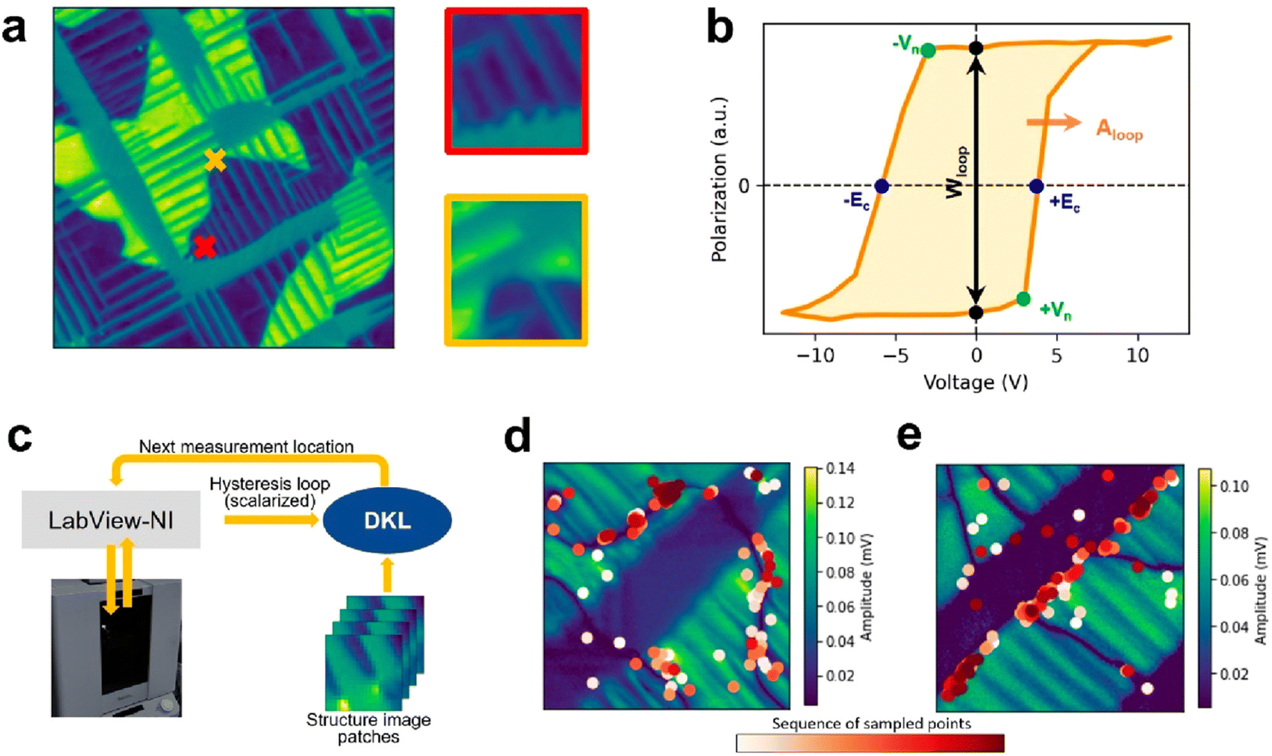 | ||
| Fig. 6 Deep kernel learning (DKL) applied to identify the microstructural origins of ferroelectricity in PbTiO3. (a) A piezoresponse force microscopy image obtained over a large field of view is split into a series of patches. (b) A voltage–polarization hysterisis spectrum measured at a patch is converged into a single scalar used in the optimisation. (c) The DKL model learns to map between the image patch and the scalarised output. (d) and (e) Examples of DKL sampled points during the optimisation, highlighting the order the points were sampled. Reproduced with permission from Ziatdinov et al.68 | ||
Accelerated computations
Bayesian optimisation has been widely employed to optimise the discovery of new materials in computational screenings. Nanoporous materials are developing technologies used to store, capture and sense gases. Given a target molecule, a typical task is to search a large library of materials to find the one with optimal adsorption properties. However, the current cost of such searches, either experimentally or computationally, is relatively high and limits the number of systems that can be studied. Deshwal et al.70 applied Bayesian optimisation to search a database of ∼70000 hypothetical covalent organic frameworks (COFs) for the system with the highest simulated methane deliverable capacity. Their Bayesian optimisation approach identified ∼30% of the top 100 ranked COFs after evaluating only 140 systems, including identifying the optimal material in the dataset. Lampe et al.71 integrated three machine-learning models with Bayesian optimisation, and successfully achieved precise control over CsPbBr3 nanoplatelet thickness with enhanced optical quality and monodispersity with minimal data requirements. The algorithm's ability to optimise spectral quality, account for purity, and incorporate heuristic constraints enabled rapid improvement, achieving remarkable results with only 220 samples for nanoplatelet syntheses, orders of magnitude fewer than necessary for other complex approaches. Seko et al.72 used Bayesian optimisation with the Kriging method73 to discover materials with low lattice thermal conductivity (κl) for thermoelectric applications. They explored over 50000 potential materials using an initial dataset of 101 first-principles anharmonic lattice dynamics calculations. Their study identified 21 materials with low lattice thermal conductivities suitable for high-performance thermoelectrics, including two compounds with κl less than 0.5 W m−1 K at 300 K and a narrow electronic band gap less than 1 eV.
Needle-in-a-haystack problems, in which the optimum value appears in a small portion of the total search space, exist across a wide range of fields including disease prediction and materials property optimisation. The problems typically pose a challenge to Bayesian optimisation algorithms which exhibit slow convergence or get stuck in local optima. Siemenn et al.74 developed a new approach they termed the Zooming Memory-Based Initialization algorithm (ZoMBI) to tackle needle-in-a-haystack problems building on traditional Bayesian optimisation. Their approach starts by iteratively zooming in on the manifold search bounds, with each dimension handled independently, using a set number of memory points to identify the plausible region containing the global optimum needle. Next, the memory points not being used to zoom in the search bounds are pruned to reduce the computational cost. In an approach that better mimics the human learning process, actively learned acquisition function hyperparameters are used to tune the preference between exploration and exploitation. Together, these procedures enable the optimisation method to locate the region containing the optimum needle and avoid local optima. The method was benchmarked on two real-world problems, namely identifying materials with a highly negative Poisson's ratio and materials with a highly positive thermoelectric figure of merit, for which exhaustive computational datasets were available. They find the ZoMBI algorithm outperforms standard Bayesian optimisation (a computational speed-up of 400×) and other state-of-the-art algorithms designed for needle-in-a-haystack problems (3× fewer experiments).
Machine-learning interatomic potentials (MLIPs) have emerged as efficient surrogate models for approximating ab initio potential energy surfaces. However, computational searches employing MLIPs are constrained by their reduced accuracy, particularly for out-of-sample predictions of energies and forces on unseen regions of composition or configuration space. Tran et al.75 developed a multi-fidelity machine learning framework to fuse a hierarchy of atomistic computational models, with density functional theory calculations and a SNAP MLIP76 used for high- and low-fidelity predictions, respectively.77,78 By coupling their model to a Bayesian optimisation procedure, they performed an on-the-fly search for materials with high bulk modulus in the Al–Nb–Ti ternary composition space. Their approach was able to locate the optimum material after only 5 high-fidelity and 31 low-fidelity evaluations, demonstrating the power of multi-fidelity inference coupled with Bayesian optimisation.
Challenges and opportunities
While the utility of Bayesian optimisation in the physical sciences has been demonstrated, further developments are required to increase its robustness to real data and the scaling to more complex problems of interest to chemists.Noisy data
In most practical optimisation tasks, the objective function evaluation is subject to random noise, for example, due to errors arising from the instrumental resolution or inhomogeneity of prepared samples. To illustrate the impact of noise on the Bayesian optimisation procedure, we investigate applying random fluctuations to the two-dimensional Rastrigin function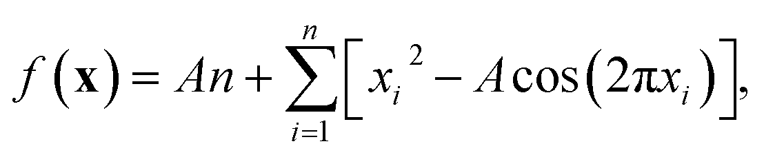 | (18) |
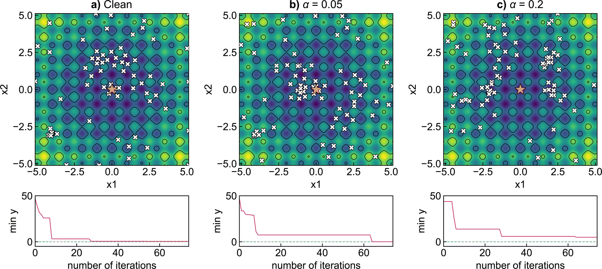 | ||
| Fig. 7 The impact of noise on the optimisation of the two-dimensional Rastrigin function, a non-linear, non-convex function with many minima. Noise is simulated by adding a random vector to the model inputs, with variance α. Bayesian optimisation finds the global minimum in the case of (a) clean data (α = 0) and (b) low noise (α = 0.05) but fails for (c) high noise (α = 0.2). | ||
To improve the robustness of optimisation algorithms on noisy tasks, Aldeghi et al.56 developed the Golem approach, which accounts for sources of uncertainty and reweights the merits of previous experiments. Golem explicitly models the objective function uncertainty with parametric probability distributions that assign a weight to the collected measurements. This allows the construction of an objective function that maximises the average performance under variable conditions, while penalizing the expected variance of the results. This new surrogate model is highly correlated with the true robust objective, therefore, the predictions made by Golem exhibit increased accuracy and are useful in problems even with high levels of noise. This approach is designed to be agnostic to the experiment planning strategy or optimisation algorithm and is therefore useful in contexts beyond Bayesian optimisation. They benchmark their approach on synthetic optimisation tasks, including analytical chemistry protocols under noisy experimental conditions, finding considerable efficiency improvements in both systematic searches and those powered by Bayesian optimisation. An alternative approach was proposed by Noack et al.79 who highlight the importance of accounting for inhomogeneous noise (not independent and identically distributed noise). The general solution they adopt is to estimate and model noise through the Gaussian process directly as
 | (19) |
 | (20) |
Parallel optimisation
For high-dimensional tasks, parallel optimisation can improve the accuracy, convergence, and overall performance of the optimisation process. In contrast to batch optimisation, where points are chosen for evaluation sequentially in each iteration,80 parallel optimisation involves conducting multiple optimisation processes simultaneously from various starting points across different partitions of the search space. The simplest approach of this sort is multi-start gradient descent. In this method, the initial points are distributed randomly with space-filling techniques and gradient descent performed independently for each starting point. During optimisation, the points will fall into their local minima automatically, without the need for explicit space partitioning. However, this approach is limited to situations where the optimisation function is known and is differentiable or where it is feasible to calculate the derivatives by numerical methods. Furthermore, this method relies on at least one initial point being placed within the basin of the true global minimum, since the algorithm lacks the capability for global exploration.More advanced techniques have been developed that are suitable for Bayesian optimisation. One method is the bandit greedy-selection approach, which aims to allocate limited resources between competing choices.81 Bandit methods are often used in conjunction with Thompson sampling, a heuristic algorithm to balance the exploration and exploitation rates in multi-armed bandit problems. The underlying logic is how to choose the most efficient sampling points according to the optimal probability. Ueno et al.32 developed a Python package (COMBO) employing Thompson sampling, random feature maps, one-rank Cholesky updates, and automatic hyperparameter tuning for Bayesian optimisation, and applied it to discover the atomic structure of a crystalline interface. Furthermore, Kandasamy et al.82 explored variations of the classical Thompson sampling process combined with Bayesian optimisation for parallel computing. Their study highlighted that operating n iterations distributed among T workers can provide a similar performance as if n sequential operations were made.
Building on these methods, Falkner et al.83 introduced the Bayesian optimisation and HyperBand approach (BOHB). HyperBand aims to speed up the searching process by spreading the initial starting points over different partitions of the parameter space and performing multiple Bayesian optimisation processes at the same time.84 After several iterations, the worst-performing optimisation processes are stopped, where the fraction stopped is an adjustable hyperparameter, and the other processes allowed to continue, with the stopping stage repeated until there is only one worker left. In their benchmarks, they demonstrated the algorithm exhibits enhanced efficiency throughout the entire learning process and identifies the global minimum with 40% fewer objective evaluations compared to standard Bayesian optimisation. Furthermore, it allows the utilisation of parallel computing techniques which further decrease the computational time.
Multi-objective optimisation
When optimising for more than one parameter of interest, multi-objective Bayesian optimisation (MBO) is an attractive method.85,86 A typical example might include finding optimal solutions for stability as well as a functional property quantifying overall performance.87–90 In the traditional Bayesian optimisation algorithm, the N best solutions generated by prior calculations are used to rebuild the probabilistic model. For multi-objective problems, it is challenging to decide on the “best” solution and one must develop a ranking scheme to weight individual parameters in the overall score. Non-dominated sorting is a key concept that originated from multi-objective evolutionary algorithms91 and is widely applied as target ranking schemes in multi-objective Bayesian optimisation. It accounts for a significant proportion of the computational cost when applying selection, comparison and crossover.92,93 A multitude of non-dominated sorting methods have been proposed and must be carefully selected based on the functional space in chemical and materials science.Agarwal et al.94 applied multi-objective Bayesian optimisation to the discovery of benzothiadiazole (BzNSN) redoxmers, with the goal of simultaneously optimising the reduction potential, solvation-free energy, and absorption wavelength. They applied their approach to a dataset of 1400 BzNSN molecules, where properties were calculated using density functional theory calculations. They demonstrated at least 15 times increased efficiency compared to randomly selecting materials highlighting the flexibility for the discovery of functional materials.
The main difficulty in multi-objective optimisation is balancing different target properties to maximise the use of available data. For physical experiments, the cost of measuring different properties can vary substantially. For example, optical properties can often be measured efficiently through in situ spectroscopic techniques, whereas surface morphology requires more laborious experimental procedures. It is desirable to first explore the objectives with lower to locate regions with suitable values, before continuing the search across more expensive objectives within these regions. This procedure can reduce the overall cost and the initial data can be applied to design a new target space with less complexity by dimension reduction. Further cost reductions can be achieved by combining multi-objective Bayesian optimisation with parallel search methods.
Integration of chemical knowledge
In some fields, black-box optimisation starting from no prior information is necessary. In the chemistry domain however, we generally have some insights and expectations concerning the physical nature of our system and its variables. For Bayesian optimisation, this may involve the incorporation of physical laws, phase stability criteria, and intrinsic material property constraints to inform the surrogate model/acquisition function and refine the search towards regions most likely to contain promising solutions. The integration of a structured probabilistic model that captures the expected physical behavior of the system proved successful for solving Ising problems in physics.95 Constrained Bayesian optimisation was used to improve the validity and quality of molecular candidates in a generative computational search.96 In the context of materials design, leveraging information on preferred coordination environments, valency, and known synthetic accessibility, could guide the optimisation process to consider only chemically viable compositions and structures. The challenge to realise this opportunity lies in developing methods to encode such qualitative knowledge into quantitative, algorithmically processable constraints without oversimplifying the problem and limiting the diversity of emerging solutions. An optimal solution may deviate from our expectations based on known chemistries.Chemistry- or physics-driven models can help navigate vast combinatorial spaces for materials design. Häse et al.97 developed Gryffin to accelerate the search for promising materials by incorporating Bayesian optimisation with smooth approximations to categorical distributions and physicochemical descriptors. The approach was used to design non-fullerene acceptors for organic solar cells, hybrid organic–inorganic perovskites for light-harvesting, and ligands and process parameters for Suzuki–Miyaura reactions. Inclusion of domain knowledge was found to lead to a superior strategy for mixed categorical-continuous optimisation in chemistry and materials science compared to state-of-the-art methods such as one-hot encoding. Clancy and co-workers developed the Physical analytics pipeLine98 (PAL) and PAL 2.0 (ref. 99) approaches that merge physics-based models with Bayesian optimisation using a physics-based prior mean for the Gaussian process surrogate model. Physical descriptors correlated to the target property were identified by XGBoost and used as features for a neural network to predict the prior mean. They found PAL 2.0 could obtain lower prediction errors for unseen material compositions in the design of metal halide perovskites and organic thermoelectric semiconductors than off-the-shelf Bayesian optimisation packages and one-hot-encoded Gaussian process methods. Chemical knowledge can further be introduced through automated experiments or ab initio calculations. Sun et al.100 demonstrated a sequential learning framework with physics constraints from high-throughput degradation tests and first-principle calculations of phase thermodynamics to identify the most stable alloyed multi-cation perovskites. Superior search efficiency was demonstrated by identifying the Cs0.17MA0.03FA0.80PbI3 (MA = methylammonium, FA = formamidinium) perovskite composition with minimal optical change under increased temperature, moisture, and illumination. This compound exhibited a 17-fold stability improvement compared to well-known CH3NH3PbI3, despite the method only sampling 1.8% of the discretised compositional space. In related work, Pedersen et al.101 combined a kinetic model based on density functional theory and Bayesian optimisation to predict the most efficient compositions for the oxygen reduction reaction in high-entropy alloys (HEAs). The model identified the optimal compositions of Ag15Pd85 and Ir50Pt50, and successfully extrapolated to other binary alloys.
Conclusion
We have introduced the strategy of Bayesian optimisation for accelerating discoveries in the chemistry domain. The key concepts are a surrogate model to estimate the probability distribution of the unseen objective function and an acquisition function to determine which point to sample next. We compared the performance of numerical (gradient descent), heuristic (simulated annealing) and statistical approaches (Bayesian optimisation) on toy optimisation problems, highlighting the potential for significant efficiency gains.Bayesian optimisation is being adopted to aid the discovery of optimal molecules/materials and accelerate experimental characterisation of structures and properties. Despite this progress in the application of statistical optimisation methods, several challenges and opportunities remain. Real experimental data is often noisy and this must be considered for efficient searches. In many setups, evaluating a sample can be highly costly and involve multiple observables. Parallel and multi-objective optimisation approaches have been developed that can overcome such challenges but currently require careful consideration of hyperparameters tailored for specific problems. An understanding of the range of chemical problems and the suitable methods in each case will facilitate the general application of Bayesian optimisation in chemical discoveries.
Conflicts of interest
There are no conflicts to declare.Acknowledgements
We thank Sterling Baird for useful suggestions of optimisation packages and maintenance of the https://github.com/AccelerationConsortium/awesome-self-driving-labs list. A. M. G. was supported by EPSRC Fellowship EP/T033231/1. We are grateful to the UK Materials and Molecular Modelling Hub for computational resources, which are partially funded by EPSRC (EP/T022213/1, EP/W032260/1 and EP/P020194/1).References
- S. W. Krska, D. A. DiRocco, S. D. Dreher and M. Shevlin, The evolution of chemical high-throughput experimentation to address challenging problems in pharmaceutical synthesis, Acc. Chem. Res., 2017, 50, 2976–2985 CrossRef CAS PubMed.
- N. K. Jangid, S. Jadoun and N. Kaur, A review on high-throughput synthesis, deposition of thin films and properties of polyaniline, Eur. Polym. J., 2020, 125, 109485 CrossRef.
- A. G. Wills, S. Charvet, C. Battilocchio, C. C. Scarborough, K. M. Wheelhouse, D. L. Poole, N. Carson and J. C. Vantourout, High-throughput electrochemistry: state of the art, challenges, and perspective, Org. Process Res. Dev., 2021, 25, 2587–2600 CrossRef CAS.
- A. Buitrago Santanilla, E. L. Regalado, T. Pereira, M. Shevlin, K. Bateman, L.-C. Campeau, J. Schneeweis, S. Berritt, Z.-C. Shi and P. Nantermet, et al., Nanomole-scale high-throughput chemistry for the synthesis of complex molecules, Science, 2015, 347, 49–53 CrossRef CAS PubMed.
- B. J. Shields, J. Stevens, J. Li, M. Parasram, F. Damani, J. I. M. Alvarado, J. M. Janey, R. P. Adams and A. G. Doyle, Bayesian reaction optimization as a tool for chemical synthesis, Nature, 2021, 590, 89–96 CrossRef CAS PubMed.
- A. O. Oliynyk, E. Antono, T. D. Sparks, L. Ghadbeigi, M. W. Gaultois, B. Meredig and A. Mar, High-throughput machine-learning-driven synthesis of full-Heusler compounds, Chem. Mater., 2016, 28, 7324–7331 CrossRef CAS.
- W. Gao, P. Raghavan and C. W. Coley, Autonomous platforms for data-driven organic synthesis, Nat. Commun., 2022, 13, 1–4 CAS.
- E. K. Chong and S. H. Zak, An introduction to optimization, John Wiley & Sons, 2004 Search PubMed.
- J. Snoek, H. Larochelle and R. P. Adams, Practical Bayesian optimization of machine learning algorithms, Advances in Neural Information Processing Systems, 2012, 25, 2960–2968 Search PubMed.
- C. A. Floudas and P. M. Pardalos, Optimization in computational chemistry and molecular biology: local and global approaches, Springer Science & Business Media, 2000, vol. 40 Search PubMed.
- S. Ruder, An overview of gradient descent optimization algorithms, arXiv, 2016, preprint arXiv:1609.04747, DOI:10.48550/arXiv.1609.04747.
- H. A. Abbass, R. Sarker and C. S. Newton, Data Mining: A Heuristic Approach: A Heuristic Approach, IGI Global, 2001 Search PubMed.
- S. Kirkpatrick, C. D. Gelatt Jr and M. P. Vecchi, Optimization by simulated annealing, Science, 1983, 220, 671–680 CrossRef CAS PubMed.
- J. H. Holland, Genetic algorithms, Sci. Am., 1992, 267, 66–73 CrossRef.
- T. Krink, J. S. VesterstrOm and J. Riget, Particle swarm optimisation with spatial particle extension, in Proceedings of the 2002 Congress on Evolutionary Computation (CEC'02), cat. no. 02TH8600, 2002, pp. 1474–1479 Search PubMed.
- L. M. Gambardella, É. D. Taillard and M. Dorigo, Ant colonies for the quadratic assignment problem, J. Oper. Res. Soc., 1999, 50, 167–176 CrossRef.
- P. Dangeti, Statistics for machine learning, Packt Publishing Ltd, 2017 Search PubMed.
- P. V. Kumar and Y. Jin, Bayesian Optimisation for Efficient Material Discovery: A Mini Review, Nanoscale, 2023, 10975–10984 Search PubMed.
- B. Shahriari, K. Swersky, Z. Wang, R. P. Adams and N. De Freitas, Taking the human out of the loop: a review of Bayesian optimization, Proc. IEEE, 2015, 104, 148–175 Search PubMed.
- S. M. Moosavi, K. M. Jablonka and B. Smit, The role of machine learning in the understanding and design of materials, J. Am. Chem. Soc., 2020, 142, 20273–20287 CrossRef CAS PubMed.
- T. Bayes, LII. An essay towards solving a problem in the doctrine of chances. By the late Rev. Mr. Bayes, FRS communicated by Mr. Price, in a letter to John Canton, AMFR S, Philos. Trans. R. Soc. London, 1763, 370–418 Search PubMed.
- C. M. Grinstead and J. L. Snell, Introduction to probability, American Mathematical Soc., 1997 Search PubMed.
- T. L. Lincoln and R. D. Parker, Medical diagnosis using Bayes theorem, Health Serv. Res., 1967, 2, 34 Search PubMed.
- J. Močkus, On Bayesian methods for seeking the extremum, in Optimization Techniques IFIP Technical Conference, 1975, pp. 400–404 Search PubMed.
- J. B. Mockus and L. J. Mockus, Bayesian approach to global optimization and application to multiobjective and constrained problems, J. Optim. Theor. Appl., 1991, 70, 157–172 CrossRef.
- P. I. Frazier, A tutorial on Bayesian optimization algorithms, arXiv, 2018, preprint, arXiv:1807.02811, DOI:10.48550/arXiv.1807.02811.
- S. Greenhill, S. Rana, S. Gupta, P. Vellanki and S. Venkatesh, Bayesian optimization for adaptive experimental design: a review, IEEE Access, 2020, 8, 13937–13948 Search PubMed.
- S. Baird, Honegumi, 2023, https://github.com/sgbaird/honegumi.
- L. D. González and V. M. Zavala, New paradigms for exploiting parallel experiments in Bayesian optimization, Comput. Chem. Eng., 2023, 170, 108110, DOI:10.1016/j.compchemeng.2022.108110.
- F. Nogueira, Bayesian optimization: open source constrained global optimization tool for Python, 2014, https://github.com/fmfn/BayesianOptimization Search PubMed.
- M. Balandat, B. Karrer, D. R. Jiang, S. Daulton, B. Letham, A. G. Wilson and E. Bakshy, BoTorch: A Framework for Efficient Monte-Carlo Bayesian Optimization, Adv. Neural Inf. Process. Syst., 2020, 33, 21524–21538 Search PubMed.
- T. Ueno, T. D. Rhone, Z. Hou, T. Mizoguchi and K. Tsuda, COMBO: an efficient Bayesian optimization library for materials science, Mater. Discovery, 2016, 4, 18–21 CrossRef.
- K. Kandasamy, K. R. Vysyaraju, W. Neiswanger, B. Paria, C. R. Collins, J. Schneider, B. Poczos and E. P. Xing, Tuning Hyperparameters without Grad Students: Scalable and Robust Bayesian Optimisation with Dragonfly, J. Mach. Learn. Res., 2020, 21, 1–27 Search PubMed.
- GPyOpt: A Bayesian Optimization Framework in Python, 2016, http://github.com/SheffieldML/GPyOpt.
- J. Bergstra, D. Yamins and D. Cox, Making a science of model search: hyperparameter optimization in hundreds of dimensions for vision architectures, in International conference on machine learning, 2013, pp. 115–123 Search PubMed.
- Y. Wang, T.-Y. Chen and D. G. Vlachos, NEXTorch: a design and Bayesian optimization toolkit for chemical sciences and engineering, J. Chem. Inf. Model., 2021, 61, 5312–5319, DOI:10.1021/acs.jcim.1c00637.
- T. Akiba, S. Sano, T. Yanase, T. Ohta and M. Koyama, Optuna: A Next-generation Hyperparameter Optimization Framework, in Proceedings of the 25rd ACM SIGKDD International Conference on Knowledge Discovery and Data Mining, 2019 Search PubMed.
- T. Head, M. Kumar, H. Nahrstaedt, G. Louppe and I. Shcherbatyi, Scikit-optimize/scikit-optimize, Zenodo, 2020, 4014775 Search PubMed.
- M. Lindauer, K. Eggensperger, M. Feurer, A. Biedenkapp, D. Deng, C. Benjamins, T. Ruhkopf, R. Sass and F. Hutter, SMAC3: A Versatile Bayesian Optimization Package for Hyperparameter Optimization, Journal of Machine Learning Research, 2022, 23, 1–9 Search PubMed.
- M. A. Ziatdinov, et al. , Mach. Learn.: Sci. Technol., 2022, 3, 015003, DOI:10.1088/2632-2153/ac4baa.
- M. Ziatdinov, Y. Liu, A. N. Morozovska, E. A. Eliseev, X. Zhang, I. Takeuchi, S. V. Kalinin, Hypothesis learning in an automated experiment: application to combinatorial materials libraries, arXiv, 2021, preprint, arXiv:2112.06649.
- R. Hickman, M. Sim, S. Pablo-García, I. Woolhouse, H. Hao, Z. Bao, P. Bannigan, C. Allen, M. Aldeghi and A. Aspuru-Guzik, Atlas: A Brain for Self-driving Laboratories, 2023 Search PubMed.
- M. Todorović, M. U. Gutmann, J. Corander and P. Rinke, Bayesian inference of atomistic structure in functional materials, npj Comput. Mater., 2019, 5, 35, DOI:10.1038/s41524-019-0175-2.
- R.-R. Griffiths, L. Klarner, H. B. Moss, A. Ravuri, S. Truong, B. Rankovic, Y. Du, A. Jamasb, J. Schwartz, A. Tripp, et al., GAUCHE: a library for Gaussian processes in chemistry, arXiv, 2022, preprint, arXiv:2212.04450, DOI:10.48550/arXiv.2212.04450.
- M. Diessner, K. Wilson and R. D. Whalley, NUBO: A Transparent Python Package for Bayesian Optimisation algorithms, arXiv, 2023, preprint, arXiv:2305.06709, DOI:10.48550/arXiv.2305.06709.
- F. Häse, M. Aldeghi, R. J. Hickman, L. M. Roch, M. Christensen, E. Liles, J. E. Hein and A. Aspuru-Guzik, Olympus: a benchmarking framework for noisy optimization and experiment planning, Mach. Learn.: Sci. Technol., 2021, 2, 035021 Search PubMed.
- F. Hase, L. M. Roch, C. Kreisbeck and A. Aspuru-Guzik, Phoenics: a Bayesian optimizer for chemistry, ACS Cent. Sci., 2018, 4, 1134–1145 CrossRef CAS PubMed.
- K. Felton, J. Rittig and A. Lapkin, Summit: Benchmarking Machine Learning Methods for Reaction Optimisation, Chem. Methods, 2021, 116–122 CrossRef CAS.
- M. Seeger, Gaussian processes for machine learning, Int. J. Neural Syst., 2004, 14, 69–106 CrossRef.
- L. Breiman, Random forests, Mach. Learn., 2001, 45, 5–32 CrossRef.
- F. Hutter, L. Xu, H. H. Hoos and K. Leyton-Brown, Algorithm runtime prediction: methods & evaluation, Artif. Intell., 2014, 206, 79–111 CrossRef.
- J. R. Quinlan, Induction of decision trees, Mach. Learn., 1986, 1, 81–106 Search PubMed.
- T. K. Ho, Random decision forests, in Proceedings of 3rd International Conference on Document Analysis and Recognition, 1995, pp. 278–282 Search PubMed.
- C. Williams and C. Rasmussen, Gaussian processes for regression, Adv. Neural Inf. Process. Syst., 1995, 8, 514–520 Search PubMed.
- J.-C. Lévesque, A. Durand, C. Gagné and R. Sabourin, Bayesian optimization for conditional hyperparameter spaces, in 2017 International Joint Conference on Neural Networks (IJCNN), 2017, pp. 286–293 Search PubMed.
- M. Aldeghi, F. Häse, R. J. Hickman, I. Tamblyn and A. Aspuru-Guzik, Golem: an algorithm for robust experiment and process optimization, Chem. Sci., 2021, 12, 14792–14807 RSC.
- J. P. Becque and D. Halliday, Modelling an optimised thin film solar cell, Eur. J. Phys., 2019, 40, 025501 CrossRef.
- C. W. Coley, N. S. Eyke and K. F. Jensen, Autonomous discovery in the chemical sciences part I: progress, Angew. Chem., Int. Ed., 2020, 59, 22858–22893 CrossRef CAS PubMed.
- Q. Liang, A. E. Gongora, Z. Ren, A. Tiihonen, Z. Liu, S. Sun, J. R. Deneault, D. Bash, F. Mekki-Berrada and S. A. Khan, et al., Benchmarking the performance of Bayesian optimization across multiple experimental materials science domains, npj Comput. Mater., 2021, 7, 1–10 CrossRef.
- C. Li, D. Rubín de Celis Leal, S. Rana, S. Gupta, A. Sutti, S. Greenhill, T. Slezak, M. Height and S. Venkatesh, Rapid Bayesian optimisation for synthesis of short polymer fiber materials, Sci. Rep., 2017, 7, 1–10 CrossRef PubMed.
- T. Hardwick and N. Ahmed, Digitising chemical synthesis in automated and robotic flow, Chem. Sci., 2020, 11, 11973–11988 RSC.
- J. Lofgren, D. Tarasov, T. Koitto, P. Rinke, M. Balakshin and M. Todorovic, Machine learning optimization of lignin properties in green biorefineries, ACS Sustain. Chem. Eng., 2022, 10, 9469–9479 CrossRef CAS.
- M. A. Carreira-Perpinán, A review of dimension reduction techniques, in Department of Computer Science, University of Sheffield, Tech. Rep. CS-96-09, 1997, vol. 9, pp. 1–69 Search PubMed.
- R. J. Lygoe, M. Cary and P. J. Fleming, A real-world application of a many-objective optimisation complexity reduction process, in International Conference on Evolutionary Multi-Criterion Optimization, 2013, pp. 641–655 Search PubMed.
- C. B. Wahl, M. Aykol, J. H. Swisher, J. H. Montoya, S. K. Suram and C. A. Mirkin, Machine learning-accelerated design and synthesis of polyelemental heterostructures, Sci. Adv., 2021, 7, eabj5505 CrossRef CAS PubMed.
- G. Binnig, C. F. Quate and C. Gerber, Atomic force microscope, Phys. Rev. Lett., 1986, 56, 930 CrossRef PubMed.
- I.-J. Chen, M. Aapro, A. Kipnis, A. Ilin, P. Liljeroth and A. S. Foster, Precise atom manipulation through deep reinforcement learning, Nat. Commun., 2022, 13, 7499 CrossRef CAS PubMed.
- M. Ziatdinov, Y. Liu, K. Kelley, R. Vasudevan and S. V. Kalinin, Bayesian active learning for scanning probe microscopy: from Gaussian processes to hypothesis learning, ACS Nano, 2022, 16, 13492–13512 CrossRef CAS PubMed.
- Y. Liu, K. P. Kelley, R. K. Vasudevan, H. Funakubo, M. A. Ziatdinov and S. V. Kalinin, Experimental discovery of structure–property relationships in ferroelectric materials via active learning, Nature Machine Intelligence, 2022, 4, 341–350 CrossRef.
- A. Deshwal, C. M. Simon and J. R. Doppa, Bayesian optimization of nanoporous materials, Mol. Syst. Des. Eng., 2021, 6, 1066–1086 RSC.
- C. Lampe, I. Kouroudis, M. Harth, S. Martin, A. Gagliardi and A. S. Urban, Rapid Data-Efficient Optimization of Perovskite Nanocrystal Syntheses through Machine Learning Algorithm Fusion, Adv. Mater., 2023, 35, 2208772 CrossRef CAS PubMed.
- A. Seko, A. Togo, H. Hayashi, K. Tsuda, L. Chaput and I. Tanaka, Prediction of low-thermal-conductivity compounds with first-principles anharmonic lattice-dynamics calculations and Bayesian optimization, Phys. Rev. Lett., 2015, 115, 205901 CrossRef PubMed.
- M. A. Oliver and R. Webster, Kriging: a method of interpolation for geographical information systems, International Journal of Geographical Information System, 1990, 4, 313–332 CrossRef.
- A. E. Siemenn, Z. Ren, Q. Li and T. Buonassisi, Fast Bayesian optimization of Needle-in-a-Haystack problems using zooming memory-based initialization (ZoMBI), npj Comput. Mater., 2023, 9, 79 CrossRef.
- A. Tran, J. Tranchida, T. Wildey and A. P. Thompson, Multi-fidelity machine-learning with uncertainty quantification and Bayesian optimization for materials design: application to ternary random alloys, J. Chem. Phys., 2020, 153, 074705 CrossRef CAS PubMed.
- A. P. Thompson, L. P. Swiler, C. R. Trott, S. M. Foiles and G. J. Tucker, Spectral neighbor analysis method for automated generation of quantum-accurate interatomic potentials, J. Comput. Phys., 2015, 285, 316–330 CrossRef CAS.
- Y. Yang, C. Nara, X. Chen and I. Hagiwara, International Design Engineering Technical Conferences and Computers and Information in Engineering Conference, 2017 Search PubMed.
- A. Tran, T. Wildey and S. McCann, sMF-BO-2CoGP: a sequential multi-fidelity constrained Bayesian optimization framework for design applications, J. Comput. Inf. Sci. Eng., 2020, 20, 031007 CrossRef.
- M. M. Noack, G. S. Doerk, R. Li, J. K. Streit, R. A. Vaia, K. G. Yager and M. Fukuto, Autonomous materials discovery driven by Gaussian process regression with inhomogeneous measurement noise and anisotropic kernels, Sci. Rep., 2020, 10, 17663 CrossRef CAS PubMed.
- Y. Tenne and C.-K. Goh, Computational intelligence in expensive optimization problems, Springer Science & Business Media, 2010, vol. 2 Search PubMed.
- M. N. Katehakis and A. F. Veinott Jr, The multi-armed bandit problem: decomposition and computation, Math. Oper. Res., 1987, 12, 262–268 CrossRef.
- K. Kandasamy, A. Krishnamurthy, J. Schneider and B. Poczos, Asynchronous parallel Bayesian optimisation via thompson sampling algorithms, arXiv, 2017, preprint, arXiv:1705.09236, DOI:10.48550/arXiv.1705.09236.
- S. Falkner, A. Klein and F. Hutter, BOHB: robust and efficient hyperparameter optimization at scale, in International Conference on Machine Learning, 2018, pp. 1437–1446 Search PubMed.
- L. Li, K. Jamieson, G. DeSalvo, A. Rostamizadeh and A. Talwalkar, Hyperband: a novel bandit-based approach to hyperparameter optimization, J. Mach. Learn. Res., 2017, 18, 6765–6816 Search PubMed.
- P. P. Galuzio, E. H. de Vasconcelos Segundo, L. dos Santos Coelho and V. C. Mariani, MOBOpt—multi-objective Bayesian optimization, SoftwareX, 2020, 12, 100520 CrossRef.
- E. Pyzer-Knapp, G. Day, L. Chen and A. I. Cooper, Distributed multi-objective Bayesian optimization for the intelligent navigation of energy structure function maps for efficient property discovery, 2020 Search PubMed.
- G. Agarwal, H. A. Doan, L. A. Robertson, L. Zhang and R. S. Assary, Discovery of Energy Storage Molecular Materials Using Quantum Chemistry-Guided Multiobjective Bayesian Optimization, Chem. Mater., 2021, 33, 8133–8144 CrossRef CAS.
- N. Khan, D. E. Goldberg and M. Pelikan, Multi-objective Bayesian optimization algorithm, in Proceedings of the 4th Annual Conference on Genetic and Evolutionary Computation, 2002, pp. 684–684 Search PubMed.
- K. Hakhamaneshi, P. Abbeel, V. Stojanovic and A. Grover, Jumbo: scalable multi-task Bayesian optimization using offline data algorithms, arXiv, 2021, preprint, arXiv:2106.00942, DOI:10.48550/arXiv.2106.00942.
- S. R. Chowdhury and A. Gopalan, No-regret algorithms for multi-task Bayesian optimization, in International Conference on Artificial Intelligence and Statistics, 2021, pp. 1873–1881 Search PubMed.
- K. Deb, S. Agrawal, A. Pratap and T. Meyarivan, A fast elitist non-dominated sorting genetic algorithm for multi-objective optimization: NSGA-II, in International conference on parallel problem solving from nature, 2000, pp. 849–858 Search PubMed.
- H. Fang, Q. Wang, Y.-C. Tu and M. F. Horstemeyer, An efficient non-dominated sorting method for evolutionary algorithms, Evol. Comput., 2008, 16, 355–384 CrossRef PubMed.
- Q. Long, X. Wu and C. Wu, Non-dominated sorting methods for multi-objective optimization: review and numerical comparison, J. Ind. Manag. Optim., 2021, 17, 1001 Search PubMed.
- G. Agarwal, H. A. Doan, L. A. Robertson, L. Zhang and R. S. Assary, Discovery of Energy Storage Molecular Materials Using Quantum Chemistry-Guided Multiobjective Bayesian Optimization, Chem. Mater., 2021, 33, 8133–8144, DOI:10.1021/acs.chemmater.1c02040.
- M. A. Ziatdinov, A. Ghosh and S. V. Kalinin, Physics makes the difference: Bayesian optimization and active learning via augmented Gaussian process, Mach. Learn.: Sci. Technol., 2022, 3, 015003 Search PubMed.
- R.-R. Griffiths and J. M. Hernández-Lobato, Constrained Bayesian optimization for automatic chemical design using variational autoencoders, Chem. Sci., 2020, 11, 577–586 RSC.
- F. Häse, M. Aldeghi, R. J. Hickman, L. M. Roch and A. Aspuru-Guzik, Gryffin: an algorithm for Bayesian optimization of categorical variables informed by expert knowledge, Appl. Phys. Rev., 2021, 8, 031406 Search PubMed.
- H. C. Herbol, W. Hu, P. Frazier, P. Clancy and M. Poloczek, Efficient search of compositional space for hybrid organic–inorganic perovskites via Bayesian optimization, npj Comput. Mater., 2018, 4, 51 CrossRef.
- M. S. Priyadarshini, O. Romiluyi, Y. Wang, K. Miskin, C. Ganley and P. Clancy, PAL 2.0: a physics-driven Bayesian optimization framework for material discovery, Mater. Horiz., 2024, 11, 781–791 RSC.
- S. Sun, A. Tiihonen, F. Oviedo, Z. Liu, J. Thapa, Y. Zhao, N. T. P. Hartono, A. Goyal, T. Heumueller and C. Batali, et al., A data fusion approach to optimize compositional stability of halide perovskites, Matter, 2021, 4, 1305–1322 CrossRef CAS.
- J. K. Pedersen, C. M. Clausen, O. A. Krysiak, B. Xiao, T. A. Batchelor, T. Löffler, V. A. Mints, L. Banko, M. Arenz and A. Savan, et al., Bayesian optimization of high-entropy alloy compositions for electrocatalytic oxygen reduction, Angew. Chem., 2021, 133, 24346–24354 CrossRef.
Footnote |
| † Electronic supplementary information (ESI) available. See DOI: https://doi.org/10.1039/d3dd00234a |
| This journal is © The Royal Society of Chemistry 2024 |