
 Open Access Article
 This Open Access Article is licensed under a Creative Commons Attribution-Non Commercial 3.0 Unported Licence
PIGNet2: a versatile deep learning-based protein–ligand interaction prediction model for binding affinity scoring and virtual screening†
Seokhyun
Moon
 a,
Sang-Yeon
Hwang
b,
Jaechang
Lim
b and
Woo Youn
Kim
*abc
a,
Sang-Yeon
Hwang
b,
Jaechang
Lim
b and
Woo Youn
Kim
*abc
aDepartment of Chemistry, KAIST, 291 Daehak-ro, Yuseong-gu, Daejeon 34141, Republic of Korea. E-mail: wooyoun@kaist.ac.kr
bHITS Incorporation, 124 Teheran-ro, Gangnam-gu, Seoul 06234, Republic of Korea
cAI Institute, KAIST, 291 Daehak-ro, Yuseong-gu, Daejeon 34141, Republic of Korea
First published on 12th December 2023
Abstract
Prediction of protein–ligand interactions (PLI) plays a crucial role in drug discovery as it guides the identification and optimization of molecules that effectively bind to target proteins. Despite remarkable advances in deep learning-based PLI prediction, the development of a versatile model capable of accurately scoring binding affinity and conducting efficient virtual screening remains a challenge. The main obstacle in achieving this lies in the scarcity of experimental structure-affinity data, which limits the generalization ability of existing models. Here, we propose a viable solution to address this challenge by introducing a novel data augmentation strategy combined with a physics-informed graph neural network. The model showed significant improvements in both scoring and screening, outperforming task-specific deep learning models in various tests including derivative benchmarks, and notably achieving results comparable to the state-of-the-art performance based on distance likelihood learning. This demonstrates the potential of this approach to drug discovery.
1 Introduction
Predicting protein–ligand interaction (PLI) plays a critical role in the early stages of drug discovery.1–3 It can be mainly utilized for two purposes: virtual screening to efficiently identify hit candidates from a large chemical space for a target protein and a process designed to refine these discovered molecules to increase their affinities. The virtual screening emphasizes cost-effectiveness due to the extensive calculation required,4,5 while the accuracy is more important for the binding affinity improvement process due to the need for the precise evaluation of a relatively smaller number of molecules.6,7 In this light, both fast and accurate PLI prediction is necessary to meet these requirements. An ideal PLI prediction model should be computationally efficient and accurate in predicting binding affinity and thus be able to correlate the prediction with experimental binding affinities or correctly distinguish active and inactive molecules.8,9Inspired by the earlier success of machine learning-based approaches for PLI prediction,10–12 deep learning-based models have attracted great attention recently.13–16 Deep learning allowed for retaining fast computation speed while demonstrating high performance in predicting the binding affinities of protein–ligand crystal structures.17 Despite their potential, most deep learning-based PLI prediction models are insufficient to be applied to various tasks at once.18–21 Instead, they are task-specific, focusing only on scoring,16,22,23 pose optimization,24–26 or screening.27 Specifically, the scoring task is to predict the binding affinities of protein–ligand complexes, and the screening task is to classify different compounds into true binders and non-binders. Contrary to the common expectation that a model with high accuracy in binding affinity scoring will also have high accuracy in virtual screening, the performance of these two tasks is often at odds because deep learning models tend to learn exclusive (rather than generalizable) features to perform best at each task. For example, models for predicting binding affinities trained only on crystal structures performed well at scoring crystal or near-native structures but struggled with tasks such as identifying specific binders to a target protein among diverse molecules or evaluating computer-generated structures as required in virtual screening.28 Meanwhile, models that employ a Δ-learning strategy with computer-generated data27,29 or target the binding pose optimization24,25 have shown improved performance in virtual screening but failed to rank the relative binding affinities of different protein–ligand complexes adequately. These challenges underscore the difficulty in designing a versatile PLI prediction model that can effectively handle diverse tasks.
Designing a versatile deep learning-based PLI prediction model performing well on both scoring and screening is challenged by the low generalizability of the model, which is mainly due to the lack of well-curated structure-affinity data.30–32 This challenge persists despite the gradually increasing availability of binding structure data from experiments.33 To overcome this hurdle, one can impose a generalizable inductive bias throughout various tasks into the model. In the previous study, we have shown that incorporating the physics of non-covalent molecular interaction as an inductive bias improves the generalization ability of a deep learning-based PLI prediction model.34 In addition, data augmentation strategies can mitigate the problem of the lack of experimental structure-affinity data. Previous approaches adopted data augmentation strategies by training the model with docking-generated structures to predict the binding affinities of non-binding structures to be less than that of experimental structures.35,36 These strategies are based on the physical intuition that highly divergent structures of cognate ligands or structures with non-cognate ligands for a given target would have weaker binding affinities than a crystal structure of a true binder. However, models trained only with such augmented data have exhibited a relative decrease in scoring performance, diminishing their utility for this particular task.34,37
Recently, GenScore38 reported state-of-the-art performance on various tasks, including scoring and screening.‡ It is noteworthy that GenScore used neither physics-based inductive bias nor data augmentation and simply focused on learning the distance likelihood of binding structures instead of predicting their binding affinities. Direct prediction of binding affinities has the great advantage that the predicted values can be directly compared to the experimental results, allowing for an intuitive explanation and directions for further improvement, whereas distance likelihood-based results only allow for relative comparisons between predicted values.
Here, we propose a versatile deep learning-based PLI prediction model by improving its generalization ability with physics-based inductive bias and data augmentation strategy. Along with the previous data augmentation strategies, we generated near-native structures that are energetically and geometrically similar to crystal structures to consider their limited experimental resolution and intrinsic dynamic nature in vivo. The model was then trained to predict the binding affinities of these structures to be the same as the corresponding experimental values, effectively recognizing that these structures lie on the same local minima as crystal structures. As a result, PIGNet2, which is based on a physics-informed graph neural network modified from our previous work,34 showed significantly enhanced scoring and screening performance.
To demonstrate the potential applicability of PIGNet2 in scoring and screening tasks, we evaluated it against various benchmarks. We note that there are diverse machine learning and deep learning models for each benchmark with different purposes.39–43 Instead of comprehensively reviewing such existing models, our evaluation focuses on comparing PIGNet2 with the best deep learning-based PLI prediction models for each benchmark alongside traditional docking programs in the perspective of the model's versatility. We used the CASF-2016 benchmark44 to compare the overall performance on scoring, docking, and screening. Following that, we also used DUD-E45 and DEKOIS2.0 (ref. 46) as widely adopted virtual screening benchmarks to evaluate the screening performance in more detail. To further assess the scoring performance, we adopted two separate derivative benchmarks provided by Wang et al.47 and the Merck FEP benchmark,48 which will be called the derivative benchmark 2015 and 2020, respectively. Both are the structure-affinity datasets of derivative compounds with various target proteins and are specifically designed for assessing the scoring performance of PLI prediction models between structurally similar molecules. Overall, PIGNet2 outperformed task-specific models in all benchmarks, achieving results on par with the state-of-the-art performance of GenScore while leaving room for further improvement thanks to its use of intuitively explainable physics. Thus, our approach provides an alternative solution to develop a versatile deep learning model that can be used for hit identification and lead optimization in drug discovery.
2 Methods
2.1 PDBbind dataset
The PDBbind dataset,49 which comprises protein–ligand binding complex data curated from the Protein Data Bank (PDB),50 is divided into general, refined, and core sets based on the strictness of the curation. The core set is subjected to the most rigorous curation criteria, thus including representative entities with respect to a corresponding target protein. A growing trend among recent PLI prediction models is to exploit the general set in order to leverage a larger pool of crystal structures for training.35,36 This approach was inspired by a previous work demonstrating that using the larger general set can improve the performance of PLI prediction models when compared to the refined set.51In our study, however, we employed the refined set to carry out data augmentation for all the proteins and ligands with limited computational resources. This may indicate that our model still has room for improvement by expanding the number of crystal structure data with the general set. Of the 5312 complexes present in the refined set, we omitted the core set included in the CASF-2016 benchmark44 and redundant complexes. As a result, we ended up with a training set of 5046 complexes and a test set of 266 complexes. To alleviate an undesired overfitting issue possibly coming from the limited number of crystal structures, we employed data augmentation strategies as described in the next section.
2.2 Data augmentation strategies
In this section, we present our novel positive data augmentation (PDA) strategy in conjunction with various negative data augmentation (NDA) strategies: re-docking, random-docking, and cross-docking data augmentation.For PDA, we first generated 1000 conformations of each ligand using the ETKDG conformer generation method.52 We optimized those structures using the universal force field (UFF)53 and Merck molecular force field (MMFF).54 This can yield a maximum of 3000 data points for each complex. Next, the resulting structures were aligned to the ligand's pose in the crystal. Finally, the structures are minimized using the Smina docking software,55 a forked version of AutoDock Vina,56 to avoid clashes. We then selected structures that satisfy two criteria: (1) a ligand root mean square deviation (RMSD) less than 2 Å compared to the crystal structure and (2) a mean absolute error less than 1 kcal mol−1 between the Smina scores of the crystal structure and the generated structures. The latter criterion aims to select structures energetically similar to the near-native structure, in addition to the former, the geometric criterion that is more generally used. While the scoring function of Smina only approximates the PLI potential energy surface (PES), it is rational to regard structures with similar scores in a confined range as energetically near-native on the actual PES considering the continuity of energy. Finally, to remove highly similar structures that can be considered duplicates, we additionally pruned the generated structures so that the RMSD between every pair of the generated structures is greater than 0.25 Å. Along with the above, structures generated by re-docking crystal structures using Smina were also used, where the RMSD between every pair of generated structures for each complex was maintained below 2 Å.
The NDA strategies mostly follow the methods outlined in our previous work.34 However, we adopted additional guidelines here for a more rigorous generation of non-binding structures. First, the re-docking data augmentation generates structures by docking ligands into a cognate target and then extracting unstable structures. Based on the fact that crystal structures are stable binding poses, one can infer that ligand structures that deviate significantly from the crystal structure will be highly unstable. Thus, we used docking-generated structures with the ligand RMSD greater than 4 Å compared to the corresponding crystal structure. Second, cross-docking data augmentation uses the idea that a non-cognate protein–ligand pair is less likely to form a bound complex. To implement this, we grouped proteins based on a protein sequence similarity of 0.4 using the cd-hit software.58,59 Then, pairs of different protein clusters were sampled, and for each pair of clusters, proteins from one cluster were docked with ligands from the other cluster to generate structures of non-cognate protein–ligand pairs. The additional filtration criteria based on the ligand RMSD and protein sequence similarity are expected to provide stricter deviation of negatively augmented data from near-native data. Lastly, the random-docking data augmentation strategy assumes that an arbitrarily chosen molecule is unlikely to be a true binder to a given protein by chance. This was intended to incorporate a structural diversity of decoys because the re-docking and cross-docking data augmentation strategies only treat a limited number of molecules. We generated the corresponding structures by docking a random molecule from the IBS molecule dataset60 to each protein. However, as we did not add explicit rules to filter false negatives in the random-docking augmentation, we expect that a better generation strategy of decoys such as the conventional methods45,57 will improve the screening performance of the model.
For all the negative data augmentation strategies, we used Smina for docking and structure minimization and the DockRMSD61 software for calculating the ligand RMSD.
2.3 Data preprocessing
We preprocessed crystal and computer-generated structures for the PLI prediction model. Proper protonation of each molecule is crucial in this step to enhance the accurate representation of specific physical interactions such as hydrogen bonding. To this end, we protonated all the protein structures with the Reduce software.62 For the ligands, we protonated them at pH 7.4 using Dimorphite-DL.63 Water and hydrogens were removed from the complexes. As the final step, only the protein residues containing heavy atoms within 5 Å or less from the ligand were extracted and used as the protein pocket. We used RDKit,64 Open Babel,65 and PyMOL66 throughout the overall data preprocessing. A detailed breakdown of the training and test sets, derived through each data augmentation, is presented in Table 1.| Data augmentation strategy | Training set | Test set |
|---|---|---|
| PDA | 375![[thin space (1/6-em)]](https://www.rsc.org/images/entities/char_2009.gif) 184 184 |
21377 |
| NDA (re-docking) | 254163 |
12109 |
| NDA (cross-docking) | 503073 |
26470 |
| NDA (random-docking) | 957775 |
50496 |
2.4 Model architecture
PIGNet2 shares the model architecture and physics terms from our previous work34 except for the initial atom features and the van der Waals interaction term. Refer to ESI† for the modified initial atom features of PIGNet2.The overall scheme of PIGNet2 is depicted in Fig. 1. PIGNet2 works as follows. Preprocessed pocket and ligand structures with input features are first passed through a feedforward network and then through a gated graph attention network, which updates atom features based on intramolecular edges. The resulting pocket and ligand features are then passed through an interaction network, which allows the embedding of additional information from the interaction counterpart via the intermolecular edges. Finally, the pocket and ligand features are concatenated to calculate the intermolecular atom–atom pairwise interaction terms. We refer to the previous work34 for more details of the model architecture.
 | ||
| Fig. 1 The overall scheme of PIGNet2. (A) A preprocessed protein–ligand complex is sequentially fed into a gated graph attention network (GatedGAT) and an interaction network. The networks update atom features based on intra- and intermolecular edges upon each convolution, respectively. (B) Four parameterized physics terms compute intermolecular atom–atom pairwise interaction from the updated data. The total energy Epred is computed by summing all interactions for all atomic pairs, divided by a rotor penalty term Trot. Note that the architecture of PIGNet2 shares with its previous version except for the initial atom features and the van der Waals interaction (see methods for more details). | ||
The total binding affinity Epred predicted by the model is the sum of all intermolecular atom pairwise interactions consisting of four terms: EvdW, EH-bond, EMetal, and EHydrophobic. Each of them represents intermolecular van der Waals (vdW), hydrogen bond, metal–ligand, and hydrophobic interactions, respectively. In order to incorporate the effect of entropy as regularization, the total energy is divided by Trot, a term proportionate to the number of rotatable bonds of the ligand. The equation of the total energy is as follows:
 | (1) |
One feature of our current model that differs from the previous is the introduction of the Morse potential instead of the Lennard-Jones potential for EvdW. The ability of PIGNet2 to score the binding affinity of crystal structures or to clearly distinguish between active and decoy molecules is highly dependent on the modeling of the vdW potential well. For example, an overly broad potential well could result in the prediction of a degree of interaction even for atom pairs that are too far apart to contribute significantly to the interaction, resulting in predicting inherently unstable structures to be stable. On the other hand, an excessively narrow potential well could lead to the prediction of repulsive vdW interactions for atom pairs that are appropriately close, resulting in predicting unstable energies for them. The correct form of the potential well is, therefore, critical for accurate prediction. Thus, directly adjusting the potential well offers significant advantages in the design and evaluation of deep learning-based physics-informed PLI prediction models. However, the Lennard-Jones potential possesses insufficient flexibility to freely adjust the width of the potential well, which was our reason for introducing the derivative loss in the previous work.34 As a more direct and precise alternative, we chose to use the Morse potential, which allows for explicitly controlling the potential well. For an intermolecular pair of ith and jth atoms, the van der Waals interaction evdWij in terms of the Morse potential is computed as follows:
| evdWij = wij((1 − e−aij(dij−rij))2 − 1), | (2) |
2.5 Training setup
3 Results and discussion
3.1 Performance on CASF-2016 benchmark
The CASF-2016 benchmark was carefully curated from 285 protein–ligand complexes in the PDBbind core set. This benchmark provides a comprehensive set of four metrics: scoring power, ranking power, docking power, and screening power. Each metric has a unique purpose in assessing PLI prediction models.
The metrics fall into two main categories. The first category evaluates the ability of the model to predict binding affinity for crystal structures. The second category evaluates the ability of the model to distinguish true-binding structures from various computer-generated structures. Scoring power and ranking power fall into the first category, and docking power and screening power fall into the second category. The four metrics comprehensively evaluate models' performance in different aspects of PLI prediction.
Specifically, the scoring power evaluates the ability of the model to predict the binding affinity of protein–ligand crystal structures and is assessed using the Pearson correlation coefficient R. The ranking power measures the ability of the model to rank the binding affinities of protein–ligand complexes grouped by protein similarity. It is evaluated using the Spearman rank correlation coefficient ρ. The docking power assesses the ability of the model to identify near-native structures from computer-generated decoy structures. The metric is evaluated based on a top N success rate, SRN, where a case is considered successful if at least one of the top N predicted structures for each complex has a ligand root mean square deviation (RMSD) of less than 2 Å when compared to the crystal structure. Finally, the screening power evaluates the ability of the model to identify cognate protein–ligand complexes that can form a binding interaction among the vast amount of non-cognate protein–ligand complexes in cross-docking scenarios. The screening power is assessed with the top α% enrichment factor, EFα%, which is a measure of the ratio of active molecules included in the top α% model predictions to the total number of active molecules, defined as follows:
 | (3) |
DeepDock24 primarily aims to optimize protein–ligand structures. Instead of predicting binding affinities, DeepDock predicts the distance likelihood of given structures by utilizing a mixture density network67 to model the statistical potential of protein–ligand structures. GenScore,38 a model built on the same formulation as DeepDock, is trained with an additional loss term to learn the correlation between the binding affinities of different complexes. Since the authors provide ten models with different adjustable parameters and each showed different performances in various tasks, here we report the results of GT_ft_0.5 and GatedGCN_ft_1.0, which respectively showed the best performances in screening and scoring.
Unlike previous methods, OnionNet-SFCT27 and Δ-AEScore29 estimate the final energy by a linear combination of correction terms to the Autodock Vina56 scores. These methods incorporate various computer-generated structures in their training process to enhance performance in virtual screening tasks.
Finally, baseline models that directly predict exact binding affinity include AK-score,16 Sfcnn,23 OnionNet-2,22 and AEScore.29 AK-score and Sfcnn use 3D convolutional neural networks (CNN), while OnionNet-2 uses a 2D feature map with a 2D CNN. AEScore predicts binding affinities using a feedforward neural network based on an atomic environment vector representation. By including these different models in our comparison, we can thoroughly evaluate the relative performance and robustness of PIGNet2.
| Model | Prediction target | Screening power | Docking power | Scoring power | Ranking power | |
|---|---|---|---|---|---|---|
| EF1% | SR1% | SR1 | R | ρ | ||
| DeepDock24 | Distance likelihood | 16.4 | 43.9% | 89.1% | 0.460 | 0.425 |
| GenScore (GT_ft_0.5)38 | Distance likelihood | 28.2 | 71.4% | 97.6% | 0.773 | 0.659 |
| GenScore (GatedGCN_ft_1.0)38 | Distance likelihood | 23.5 | 66.1% | 95.4% | 0.834 | 0.686 |
| OnionNet-SFCT (Vina)27 | Δ binding affinity | 15.5 | — | 93.7% | 0.428 | 0.393 |
| Δ-AEScore29 | Δ binding affinity | 6.16 | 19.3% | 85.6% | 0.740 | 0.590 |
| OnionNet-2 (ref. 22) | Exact binding affinity | — | — | — | 0.864 | — |
| AEScore29 | Exact binding affinity | — | — | 35.8% | 0.830 | 0.64 |
| AK-score16 | Exact binding affinity | — | — | 36.0% | 0.812 | 0.670 |
| Sfcnn23 | Exact binding affinity | — | — | 34.0% | 0.795 | — |
| PIGNet2 | Exact binding affinity | 24.9 | 66.7% | 93.0% | 0.747 | 0.651 |
Models focusing on accurate regression of binding affinities generally demonstrate their strong performance in scoring and ranking. Nevertheless, their performance on virtual screening-related metrics lags behind those predicting distance likelihoods. Prime examples of such models include AEscore and OnionNet-2, and they have attempted to compensate for the poor screening performance by introducing various computer-generated structures and Δ-learning. Although the resulting OnionNet-SFCT and Δ-AEScore enhanced docking and screening power, their scoring and ranking powers were significantly reduced. This trend was particularly pronounced for OnionNet-SFCT, indicating that designing versatile deep learning-based PLI prediction models is challenging even with data augmentation and Δ-learning.
PIGNet2 aimed to perform equally well in all tasks using a physics-informed graph neural network coupled with various data augmentation strategies. Indeed, PIGNet2 demonstrated high performance for all metrics, comparable to the state-of-the-art performance of GenScore, while GenScore slightly outperformed PIGNet2 depending on its various versions. PIGNet2 outperformed the result of DeepDock in its primary objective, i.e., pose optimization, as shown by the docking power. Specifically, PIGNet2 attained scoring and ranking powers comparable to those of OnionNet-2, AEScore, AK-score, and Sfcnn, all of which aim to accurately score the binding affinities of crystal structures. PIGNet2 outperformed in all metrics, compared to OnionNet-SFCT and Δ-AEScore. These results support that PIGNet2 can serve as a versatile deep learning-based PLI prediction model.
3.2 Performance on classifying active and decoy compounds
While the CASF-2016 screening benchmark is well-designed and offers extensive structure data, it is different from real-world virtual screening scenarios. This is because of relatively fewer actives and decoys; the screening benchmark was curated by cross-docking between 57 protein clusters with a total of 285 protein–ligand complexes, so the number of active and decoy compounds is 5 and 280 at maximum, respectively. To evaluate the screening performance of PIGNet2 in a larger library, we used the Directory of Useful Decoys-Enhanced (DUD-E)45 and Demanding Evaluation Kits for Objective In silico Screening (DEKOIS) 2.0.46 These benchmarks comprise a much larger number of active and decoy compounds compared to CASF-2016, with a higher active-to-decoy ratio.To conduct a comparative assessment of PIGNet2 with other models, we selected the top α% enrichment factor as our primary benchmark metric, consistent with the CASF-2016 screening benchmark. We also adopted area under the receiver operating characteristic curve (AUROC)69 and Boltzmann enhanced discrimination of receiver operating characteristic curve (BEDROC)70 along with the enrichment factor. The BEDROC has an α term to adjust the criterion of early recognition, and we set it as the same value of 80.5 used in GenScore for a direct comparison. Both AUROC and BEDROC range from 0 to 1; the higher the value, the better the model's performance in classification and assigning early ranking for active compounds, respectively. Additionally, to conduct an ablation study on data augmentation in the context of screening performance, we used the Kullback–Leibler (KL) divergence, DKL.71 The KL divergence measures the deviation between the predicted binding affinity distributions, Dactive and Ddecoy, of actives and decoys, respectively, which is given as follows:
 | (4) |
The KL divergence always has a positive value, and the higher the value, the greater the deviation between Dactive and Ddecoy.
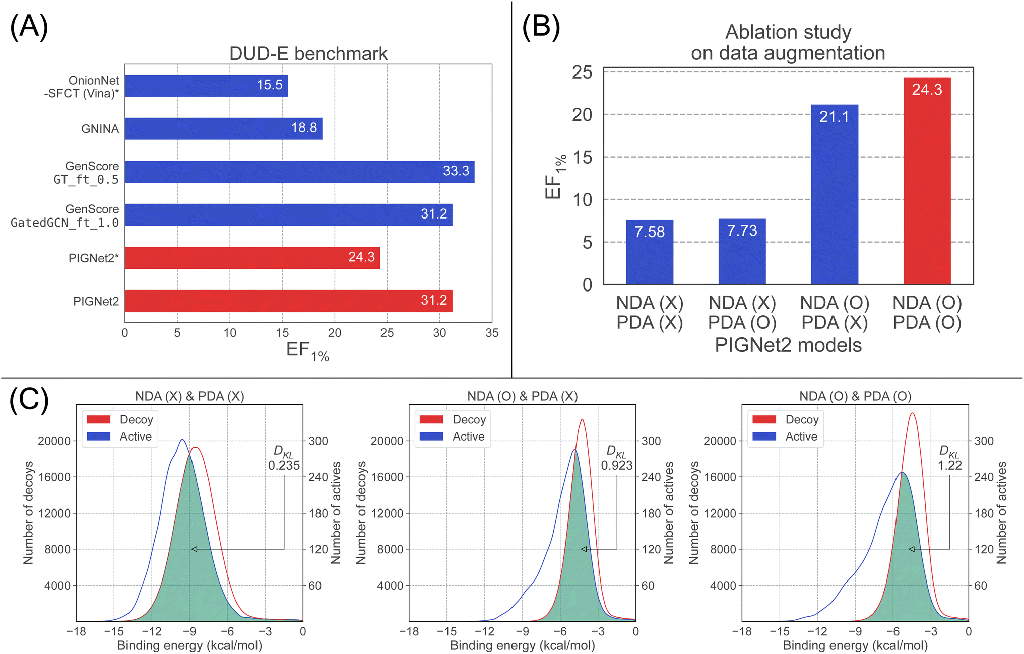 | ||
| Fig. 2 Results for the DUD-E benchmark. EF1% is the top 1% enrichment factor. (A) Comparison between baseline models and PIGNet2 in terms of the EF1%. The models with the asterisk (*), OnionNet-SFCT (Vina) and PIGNet2, used a single conformation generated by docking, while the others used multiple conformation. (B) Ablation study about data augmentation strategies for PIGNet2 on the enrichment factor of the DUD-E benchmark. We conducted all experiments in the ablation study with the same dataset used in the result of PIGNet2* in (A), which employed only the best pose prepared by Smina for each complex in the DUD-E benchmark. Each labels on x-axis means the data augmentation strategies used for training PIGNet2. For example, NDA (O) means the model trained with NDA and PDA (X) means the model trained without PDA. The red bar shows PIGNet2 model with the best performance. (C) Ablation study about data augmentation strategies for PIGNet2 on predicted distributions of actives and decoys of the DUD-E benchmark. Three models are compared: the model trained without any data augmentation strategies (left), the model trained with NDA alone (middle), and the model trained with both NDA and PDA (right). In each sub-figure, the green colored region is an overlap between the distributions of actives and decoys. | ||
To mitigate such possible biases, we further investigated the performance of PIGNet2 by using only the best pose generated by Smina and compared the results with those of OnionNet-SFCT (Vina). The resulting EF1%, 24.3, was denoted as PIGNet2* in Fig. 2(A), which was significantly dropped from the result with the top 10 structures (31.2) but is still far better than OnionNet-SFCT (Vina).
Table 3 shows the average AUROCs, BEDROC (α = 80.5), top 0.5%, 1.0%, and 5.0% enrichment factors for the DEKOIS2.0 and DUD-E benchmark. We adopted the same structures provided from Hou et al.38 since all values of the baseline models were taken from Hou et al.38. For each complex, the top ten structures were generated by Glide SP73 in the original dataset, but we further minimized them using Smina for PIGNet2. PIGNet2 outperformed Glide SP in every metric, validating its superior capability in the virtual screening task. Also, it achieved the best or second-best performance for most metrics compared to the previous state-of-the-art model, GenScore. In the case of DEKOIS2.0, PIGNet2 showed competitive performance to GenScore (GT_ft_0.5) for EF0.5%, an optimal one for screening among its various versions, while surpassing GenScore (GatedGCN_ft_1.0), an optimal model for scoring. As for AUROC, BEDROC (α = 80.5), EF1% and EF5%, PIGNet2 showed slightly better performance than both versions of GenScore. Likewise, PIGNet2 showed superior or competitive performance in the DUD-E benchmark, except for EF0.5%.
| Model | DEKOIS2.0 | DUD-E | ||||||||
|---|---|---|---|---|---|---|---|---|---|---|
| AUROC | BEDROC (α = 80.5) | EF0.5% | EF1.0% | EF5.0% | AUROC | BEDROC (α = 80.5) | EF0.5% | EF1.0% | EF5.0% | |
| Glide SP | 0.747 | 0.385 | 14.6 | 12.5 | 6.30 | 0.820 | 0.414 | 29.44 | 23.61 | 9.24 |
| GenScore (GT_ft_0.5) | 0.757 | 0.539 | 20.2 | 17.9 | 8.25 | 0.824 | 0.534 | 41.1 | 33.3 | 10.7 |
| GenScore(GatedGCN_ft_1.0) | 0.753 | 0.503 | 18.6 | 17.0 | 7.93 | 0.824 | 0.515 | 38.9 | 31.2 | 10.6 |
| PIGNet2 | 0.812 | 0.544 | 20.0 | 18.6 | 9.71 | 0.850 | 0.515 | 36.8 | 31.2 | 11.2 |
First, we observed that a model solely trained on crystal structures without both PDA and NDA exhibited no increase in EF1% after incorporating PDA. This result was expected since PDA helps the model predict affinities for near-native conformations of true binders rather than discriminating diverse decoys as NDA does. However, adding PDA to a model already improved by NDA (NDA-only model) further improved its performance compared to a model trained with NDA alone. The fact that the gain in EF1% by PDA is more prominent in the NDA-only model than in the model without both PDA and NDA indicates that PDA helps better discriminate active and decoy structures that are indistinguishable by the NDA-only model. This suggests that PDA can effectively regularize undesirable biases caused by NDA. In the comparison of the EF1% between the model with and without the data augmentation, the former performed three times better than the latter.
Next, we plotted the distribution of predicted binding affinities for the DUD-E benchmark, as shown in Fig. 2(C), to analyze how the use of each data augmentation leads to an improvement in EF1%. The model without data augmentation is on the left, the one with only NDA is in the middle, and the one with both NDA and PDA is on the right. Without the data augmentation, the two distributions have only a small deviation, indicating the discrimination between actives and decoys is difficult, resulting in a low value of EF1%. However, the deviation increased as more data augmentation strategies were applied, leading to the notable enhancement of EF1%.
Interestingly, applying NDA to the model induced a shift of both distributions to the right. This could be associated with the hinge loss used for NDA, and degraded both the screening and scoring performance. When PDA was added to the model trained with NDA, the distribution of actives shifted less than that of decoys, and hence the two distributions are more separated, particularly at high binding affinity regions. This result directly accounts for the increase in EF1%, as EF1% measures the proportion of active molecules in the top 1% of predictions.
To additionally support the analysis above, we evaluated how much the two distributions are separated in terms of DKL. A greater DKL is obviously associated with a high EF1% value since a greater DKL means a larger separation of the two distributions. As depicted in Fig. 2(C), the DKL of the model with no data augmentation, the NDA-only model, and the model with both NDA and PDA are 0.235, 0.923, and 1.22, respectively, manifesting the positive effects of NDA and PDA.
3.3 Performance on ranking structurally similar compounds
Selecting molecules with higher binding affinities to a target among plenty of similar derivatives is important during hit-to-lead and lead optimization. For this purpose, one needs to properly rank the relative binding affinities of similar molecules. However, this remains challenging due to issues such as activity cliffs, where small changes in a molecule can result in significant changes in activity.74,75 To further demonstrate the versatility of PIGNet2, we conducted a comparative analysis on derivative benchmarks.As for deep learning models, we only considered models for which the provided code can be readily applied or for which benchmark results were already available. As a result, we selected Sfcnn,23 OnionNet-SFCT (Vina),27 and GenScore.38 These models adopted different approaches, as discussed in the CASF-2016 benchmark. In summary, MM-GB/SA, Glide SP, and Smina can be categorized as traditional scoring functions, while GenScore, OnionNet-SFCT (Vina), and Sfcnn are deep learning-based PLI prediction models.
For the derivative benchmark 2015, the result of OnionNet-SFCT (Vina) was obtained by rescoring the docked structures from Autodock Vina. For both GenScore models (GT_ft_0.5 and GatedGCN_ft_1.0), we used the provided structures as-is. The results of the other models were obtained using the structures minimized by Smina. For the derivative benchmark 2020, the results of MM-GB/SA, Glide SP, and Vina were obtained from the Hou et al.38 The provided structures were generated by the flexible ligand alignment tool or glide core-constrained docking using the respective reference structure. We again minimized the given structures using Smina when evaluating PIGNet2.
| Model | Performance average R | Systems | |||||||
|---|---|---|---|---|---|---|---|---|---|
| BACE | CDK2 | JNK1 | MCL1 | p38 | PTP1B | Thrombin | TYK2 | ||
| MM-GB/SA47* | 0.40 | −0.40 | −0.53 | 0.65 | 0.42 | 0.66 | 0.67 | 0.93 | 0.79 |
| Glide SP47* | 0.29 | 0.00 | −0.56 | 0.24 | 0.59 | 0.14 | 0.55 | 0.53 | 0.79 |
| Smina55 | 0.25 | −0.48 | 0.10 | −0.060 | 0.24 | 0.52 | 0.70 | 0.72 | 0.24 |
| OnionNet-SFCT (Vina)27 | 0.023 | −0.48 | −0.68 | −0.59 | 0.29 | 0.50 | 0.66 | 0.71 | −0.23 |
| Sfcnn23 | 0.084 | −0.24 | 0.044 | −0.65 | 0.12 | 0.58 | 0.58 | 0.041 | 0.20 |
| GenScore (GT_ft_0.5)38* | 0.57 | 0.45 | 0.63 | 0.63 | 0.54 | 0.61 | 0.52 | 0.92 | 0.25 |
| GenScore (GatedGCN_ft_1.0)38* | 0.57 | 0.35 | 0.62 | 0.71 | 0.47 | 0.65 | 0.65 | 0.88 | 0.22 |
| PIGNet2 | 0.64 | 0.42 | 0.77 | 0.36 | 0.78 | 0.60 | 0.76 | 0.83 | 0.61 |
Since the derivative benchmark requires accurate prediction of the binding affinities for structurally similar derivatives, it is a much more challenging task than scoring and ranking in the CASF-2016 benchmark. OnionNet-SFCT (Vina), developed based on Δ learning focusing on virtual screening, showed anti-correlated results in almost all systems, despite its impressive docking power in the CASF-2016 benchmark. Surprisingly, Sfcnn, designed to score binding affinities accurately, performed only marginally better than OnionNet-SFCT (Vina) and poorer than traditional scoring functions. This unsatisfactory performance may be because Sfcnn, as a 3D CNN-based model, was trained exclusively on crystal structures and thus struggled to score structures optimized by Smina. Both GenScore models showed much better performances with no anti-correlation for all targets, which have a slightly lower average R value (0.57) than PIGNet2 (0.64). Furthermore, the performance of PIGNet2 in the derivative benchmark 2015, especially in terms of average R, is surprisingly close to that of PBCNet76 (0.65), a model exclusively designed for predicting the relative binding affinities of two given derivatives.
Considering the encouraging results of PIGNet2 in the derivative benchmark 2015, we expected similar success in the derivative benchmark 2020. As shown in Table 5, our model exhibited a remarkable ability compared to traditional physics-based methods. However, the average R value of PIGNet2 (0.43) was slightly lower than the best value of GenScore (0.52) while showing comparable result with the other version of GenScore (0.47). As evaluating eight targets, PIGNet2 showed positive correlations for seven systems, while a negative correlation was observed for the Eg5 system. Interestingly, a more pronounced negative correlation was observed for this particular system in other physics-based methods, suggesting that physics-based approaches may have a peculiar difficulty for this system.
| Model | Performance average R | Systems | |||||||
|---|---|---|---|---|---|---|---|---|---|
| HIF2α | PFKFB3 | Eg5 | CDK8 | SHP2 | SYK | c-Met | TNKS2 | ||
| MM-GB/SA38 | 0.35 | 0.28 | 0.55 | −0.002 | 0.65 | 0.59 | 0.11 | 0.50 | 0.16 |
| Glide SP38 | 0.30 | 0.45 | 0.48 | −0.11 | 0.35 | 0.54 | −0.006 | 0.38 | 0.32 |
| Vina38 | 0.34 | 0.49 | 0.55 | −0.52 | 0.85 | 0.57 | 0.52 | −0.26 | 0.54 |
| GenScore (GT_ft_0.5)38 | 0.47 | 0.36 | 0.45 | 0.21 | 0.67 | 0.61 | 0.23 | 0.69 | 0.54 |
| GenScore (GatedGCN_ft_1.0)38 | 0.52 | 0.52 | 0.58 | 0.21 | 0.71 | 0.61 | 0.21 | 0.73 | 0.59 |
| PIGNet2 | 0.43 | 0.45 | 0.29 | −0.09 | 0.37 | 0.72 | 0.50 | 0.57 | 0.64 |
We performed further analysis on why the anti-correlation occurred in the Eg5 system for physics-based approaches including PIGNet2. As Fig. 3 illustrates, the flexible chain in the given molecule prefers to head out to the water rather than fit into the protein pocket. It is expected that the model may less accurately predict the binding affinity of molecules that are more exposed to water, as observed in Eg5, since PIGNet2 like the other physics-based methods considers solvation effects only implicitly. Therefore, PIGNet2 predicted relatively lower binding affinities to molecules with flexible chains. This analysis highlights the great advantage of physics-based models with high explanatory power, which then provides directions for further improvement.
 | ||
| Fig. 3 Illustration of a 3D structure of Eg5-ChEMBL1085692 complex, in which the predicted binding affinity of PIGNet2 is lower than the others, resulting in a negative contribution to the correlation between predicted and experimental binding affinities. In the illustration, the transparent part is the base molecule, while the other part depicted with a ball-and-stick model is an attached flexible chain. The molecular geometries are plotted with PyMol.66 | ||
| Model | Data augmentation | Performance average R | Systems | ||||||||
|---|---|---|---|---|---|---|---|---|---|---|---|
| Negative | Positive | BACE | CDK2 | JNK1 | MCL1 | p38 | PTP1B | Thrombin | TYK2 | ||
| PIGNet2 | X | X | 0.50 | −0.16 | 0.36 | 0.21 | 0.71 | 0.67 | 0.64 | 0.82 | 0.74 |
| PIGNet2 | X | O | 0.54 | 0.23 | 0.61 | 0.33 | 0.69 | 0.64 | 0.76 | 0.66 | 0.37 |
| PIGNet2 | O | X | 0.39 | 0.085 | −0.29 | 0.25 | 0.75 | 0.45 | 0.32 | 0.82 | 0.71 |
| PIGNet2 | O | O | 0.64 | 0.42 | 0.77 | 0.36 | 0.78 | 0.60 | 0.76 | 0.83 | 0.61 |
Incorporating PDA results in maintaining or positively affecting most systems except TYK2. In this context, we have visualized the affinity prediction results for CDK2, the target where applying PDA led to the most significant performance improvement, in Fig. 4. In particular, the figure highlights a drastic change in the correlation trend from −0.29 to 0.77. This change clearly illustrates the importance of PDA in improving the scoring performance of deep learning models and in overcoming the negative effect of NDA. Consequently, using both PDA and NDA improved the scoring performance of PIGNet2 in the derivative benchmark 2015 from 0.50 to 0.64. This result implies that our data augmentation strategy undoubtedly contributed to the versatility of PIGNet2.
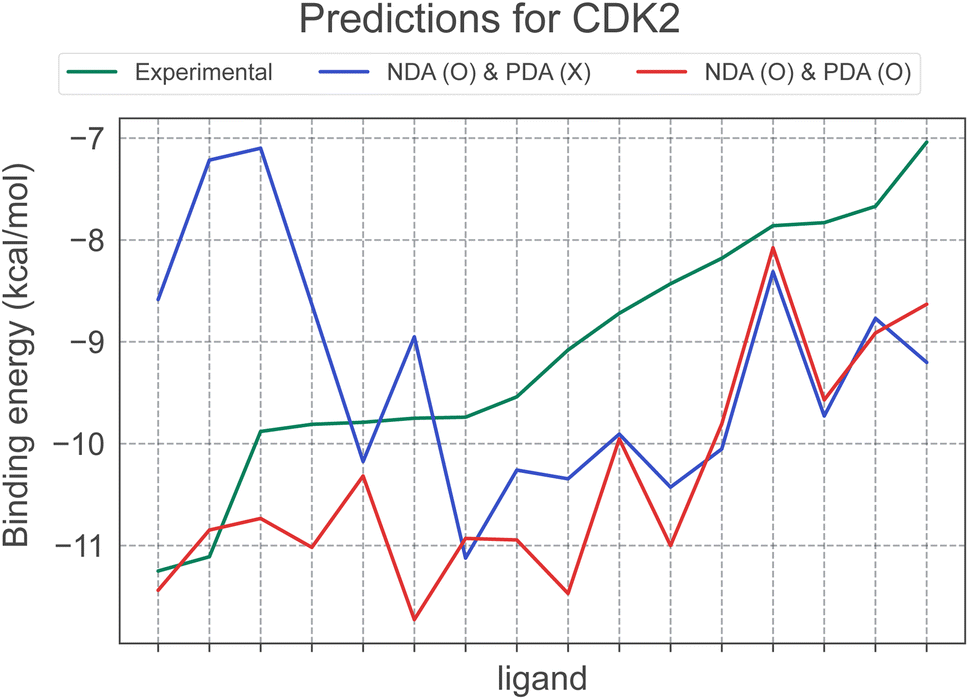 | ||
| Fig. 4 A case study for a CDK2 target system for ablation study about PDA on the derivative benchmark. The CDK2 system has 16 derivatives in total, and the illustrated result is sorted based on the experimental binding energy for all derivatives. Specifically, this figure additionally illustrates the prediction results of two models: the model trained with NDA alone and the model trained with both NDA and PDA. | ||
4 Conclusions
In this study, we present PIGNet2, a versatile deep learning-based protein–ligand interaction (PLI) prediction model that enhances its generalization ability with appropriate physics-based inductive bias and a novel data augmentation strategy called positive data augmentation (PDA) in addition to negative data augmentation (NDA). Unlike NDA, PDA generates near-native structures treated as equivalent to crystal structures during training. PIGNet2 incorporates both NDA and PDA, enabling accurate binding affinity prediction for near-native structures and effective discrimination between active and decoy molecules. Remarkably, PIGNet2 outperformed task-specific deep learning models and traditional physics-based methods in all benchmarks and is on par with the state-of-the-art performance reported recently. Furthermore, it has the distinctive advantage of predicting exact binding affinities using intuitively explainable physics, allowing for direct comparison to experimental results and providing directions for further improvement. This result solidifies the potential of PIGNet2 as a versatile deep learning-based PLI prediction model suitable for both scoring and screening tasks in drug discovery.Despite its high potential, the present method has room for further improvement. First, our generation procedure of binding structures for data augmentation would be biased toward the scoring function of the Smina docking software. This bias results in challenges when dealing with structures generated by other methods. Second, the use of NDA with the hinge loss could lead to lower predicted binding affinities for actives, as observed in the DUD-E benchmark ablation study. Third, better solvation effects should be considered to improve the prediction accuracy for molecules that are more exposed to water as observed in the benchmark result of the eg5 system. Fourth, exploring better physics terms for energy evaluation is expected to enhance the performance significantly, as the present physics terms adopted from conventional docking methods impose strong constraints in the training process and thus limit the power of deep learning. Future studies may address these issues to enhance the reliability of PLI prediction models in the drug discovery process.
Data availability
The code and trained models are available at github: https://github.com/ACE-KAIST/PIGNet2. Also, data is available at https://doi.org/10.5281/zenodo.8091220.Author contributions
Conceptualization: S. M. and W. Y. K.; methodology: S. M. and J. L.; software, investigation, and formal analysis: S. M., S.-Y. H.; writing – original draft S. M.; writing – review & editing: S. M., S.-Y. H., J. L., and W. Y. K.; supervision: W. Y. K.Conflicts of interest
There are no conflicts to declare.Acknowledgements
This work was supported by the National Research Foundation of Korea (NRF) grant funded by the Korea government (MSIT) (RS-2023-00257479).References
- O. Guvench and A. D. MacKerell, Curr. Opin. Struct. Biol., 2009, 19, 56–61 CrossRef CAS PubMed
.
- A. Masoudi-Nejad, Z. Mousavian and J. H. Bozorgmehr, In Silico Pharmacol., 2013, 1, 17 CrossRef PubMed
- N. Hansen and W. F. van Gunsteren, J. Chem. Theory Comput., 2014, 10, 2632–2647 CrossRef CAS PubMed
- B. K. Shoichet, S. L. McGovern, B. Wei and J. J. Irwin, Curr. Opin. Chem. Biol., 2002, 6, 439–446 CrossRef CAS PubMed
- J. Fan, A. Fu and L. Zhang, Quant. Biol., 2019, 7, 83–89 CrossRef CAS
- J. D. Chodera, D. L. Mobley, M. R. Shirts, R. W. Dixon, K. Branson and V. S. Pande, Curr. Opin. Struct. Biol., 2011, 21, 150–160 CrossRef CAS PubMed
- I. Muegge and Y. Hu, ACS Med. Chem. Lett., 2023, 14, 244–250 CrossRef CAS PubMed
- S.-Y. Huang, S. Z. Grinter and X. Zou, Phys. Chem. Chem. Phys., 2010, 12, 12899–12908 RSC
- H. Li, K.-H. Sze, G. Lu and P. J. Ballester, Wiley Interdiscip. Rev. Comput. Mol. Sci., 2020, 11, e1478 CrossRef
- P. J. Ballester and J. B. O. Mitchell, Bioinformatics, 2010, 26, 1169–1175 CrossRef CAS PubMed
- D. Zilian and C. A. Sotriffer, J. Chem. Inf. Model., 2013, 53, 1923–1933 CrossRef CAS PubMed
- G.-B. Li, L.-L. Yang, W.-J. Wang, L.-L. Li and S.-Y. Yang, J. Chem. Inf. Model., 2013, 53, 592–600 CrossRef CAS PubMed
- H. Öztürk, A. Özgür and E. Ozkirimli, Bioinformatics, 2018, 34, 821–829 CrossRef PubMed
- I. Lee, J. Keum and H. Nam, PLoS Comput. Biol., 2019, 15, 1–21 CrossRef PubMed
- J. Jiménez, M. Škalič, G. Martínez-Rosell and G. D. Fabritiis, J. Chem. Inf. Model., 2018, 58, 287–296 CrossRef PubMed
- Y. Kwon, W.-H. Shin, J. Ko and J. Lee, Int. J. Mol. Sci., 2020, 21, 8424 CrossRef CAS PubMed
- Z. Zhang, L. Chen, F. Zhong, D. Wang, J. Jiang, S. Zhang, H. Jiang, M. Zheng and X. Li, Curr. Opin. Struct. Biol., 2022, 73, 102327 CrossRef CAS PubMed
- J. Gabel, J. Desaphy and D. Rognan, J. Chem. Inf. Model., 2014, 54, 2807–2815 CrossRef CAS PubMed
- C. Shen, Y. Hu, Z. Wang, X. Zhang, J. Pang, G. Wang, H. Zhong, L. Xu, D. Cao and T. Hou, Brief. Bioinform., 2020, 22, bbaa070 CrossRef PubMed
- J. Yang, C. Shen and N. Huang, Front. Pharmacol., 2020, 11, 69 CrossRef CAS PubMed
- M. Su, G. Feng, Z. Liu, Y. Li and R. Wang, J. Chem. Inf. Model., 2020, 60, 1122–1136 CrossRef CAS PubMed
- Z. Wang, L. Zheng, Y. Liu, Y. Qu, Y.-Q. Li, M. Zhao, Y. Mu and W. Li, Front. Chem., 2021, 9, 753002 CrossRef CAS PubMed
- Y. Wang, Z. Wei and L. Xi, BMC Bioinf., 2022, 23, 222 CrossRef CAS PubMed
- O. Méndez-Lucio, M. Ahmad, E. A. del Rio-Chanona and J. K. Wegner, Nat. Mach. Intell., 2021, 3, 1033–1039 CrossRef
- C. Shen, X. Zhang, Y. Deng, J. Gao, D. Wang, L. Xu, P. Pan, T. Hou and Y. Kang, J. Med. Chem., 2022, 65, 10691–10706 CrossRef CAS PubMed
- Z. Wang, L. Zheng, S. Wang, M. Lin, Z. Wang, A. W.-K. Kong, Y. Mu, Y. Wei and W. Li, Brief. Bioinform., 2022, 24, bbac520 CrossRef PubMed
- L. Zheng, J. Meng, K. Jiang, H. Lan, Z. Wang, M. Lin, W. Li, H. Guo, Y. Wei and Y. Mu, Brief. Bioinform., 2022, 23, bbac051 CrossRef PubMed
- C. Shen, Y. Hu, Z. Wang, X. Zhang, J. Pang, G. Wang, H. Zhong, L. Xu, D. Cao and T. Hou, Brief. Bioinform., 2021, 22, bbaa070 CrossRef PubMed
- R. Meli, A. Anighoro, M. J. Bodkin, G. M. Morris and P. C. Biggin, J. Cheminf., 2021, 13, 59 CAS
- A. R. Leach, B. K. Shoichet and C. E. Peishoff, J. Med. Chem., 2006, 49, 5851–5855 CrossRef CAS PubMed
- K. Huang, C. Xiao, L. M. Glass and J. Sun, Bioinformatics, 2020, 37, 830–836 CrossRef PubMed
- T. Pahikkala, A. Airola, S. Pietila, S. Shakyawar, A. Szwajda, J. Tang and T. Aittokallio, Brief. Bioinform., 2014, 16, 325–337 CrossRef PubMed
- M. Volkov, J.-A. Turk, N. Drizard, N. Martin, B. Hoffmann, Y. Gaston-Mathé and D. Rognan, J. Med. Chem., 2022, 65, 7946–7958 CrossRef CAS PubMed
- S. Moon, W. Zhung, S. Yang, J. Lim and W. Y. Kim, Chem. Sci., 2022, 13, 3661–3673 RSC
- P. G. Francoeur, T. Masuda, J. Sunseri, A. Jia, R. B. Iovanisci, I. Snyder and D. R. Koes, J. Chem. Inf. Model., 2020, 60, 4200–4215 CrossRef CAS PubMed
- C. Shen, X. Hu, J. Gao, X. Zhang, H. Zhong, Z. Wang, L. Xu, Y. Kang, D. Cao and T. Hou, J. Cheminf., 2021, 13, 81 Search PubMed
- H. Li, K.-S. Leung, M.-H. Wong and P. J. Ballester, BMC Bioinform., 2016, 17, 308 CrossRef PubMed
- T. Hou, C. Shen, X. Zhang, C.-Y. Hsieh, Y. Deng, D. Wang, L. Xu, J. Wu, D. Li and Y. Kang,
et al.
, Chem. Sci., 2023, 8129–8146 Search PubMed
- Z. Cang and G.-W. Wei, PLoS Comput. Biol., 2017, 13, e1005690 CrossRef PubMed
- D. D. Nguyen and G.-W. Wei, J. Chem. Inf. Model., 2019, 59, 3291–3304 CrossRef CAS PubMed
- C. Yang and Y. Zhang, J. Chem. Inf. Model., 2022, 62, 2696–2712 CrossRef CAS PubMed
- Z. Meng and K. Xia, Sci. Adv., 2021, 7, eabc5329 CrossRef CAS PubMed
- X. Liu, H. Feng, J. Wu and K. Xia, PLoS Comput. Biol., 2022, 18, e1009943 CrossRef CAS PubMed
- M. Su, Q. Yang, Y. Du, G. Feng, Z. Liu, Y. Li and R. Wang, J. Chem. Inf. Model., 2018, 59, 895–913 CrossRef PubMed
- M. M. Mysinger, M. Carchia, J. J. Irwin and B. K. Shoichet, J. Med. Chem., 2012, 55, 6582–6594 CrossRef CAS PubMed
- M. R. Bauer, T. M. Ibrahim, S. M. Vogel and F. M. Boeckler, J. Chem. Inf. Model., 2013, 53, 1447–1462 CrossRef CAS PubMed
- L. Wang, Y. Wu, Y. Deng, B. Kim, L. Pierce, G. Krilov, D. Lupyan, S. Robinson, M. K. Dahlgren, J. Greenwood, D. L. Romero, C. Masse, J. L. Knight, T. Steinbrecher, T. Beuming, W. Damm, E. Harder, W. Sherman, M. Brewer, R. Wester, M. Murcko, L. Frye, R. Farid, T. Lin, D. L. Mobley, W. L. Jorgensen, B. J. Berne, R. A. Friesner and R. Abel, J. Am. Chem. Soc., 2015, 137, 2695–2703 CrossRef CAS PubMed
- C. E. Schindler, H. Baumann, A. Blum, D. Böse, H.-P. Buchstaller, L. Burgdorf, D. Cappel, E. Chekler, P. Czodrowski and D. Dorsch,
et al.
, J. Chem. Inf. Model., 2020, 60, 5457–5474 CrossRef CAS PubMed
- Z. Liu, M. Su, L. Han, J. Liu, Q. Yang, Y. Li and R. Wang, Acc. Chem. Res., 2017, 50, 302–309 CrossRef CAS PubMed
- H. M. Berman, Nucleic Acids Res., 2000, 28, 235–242 CrossRef CAS PubMed
- H. Li, K.-S. Leung, M.-H. Wong and P. J. Ballester, Molecules, 2015, 20, 10947–10962 CrossRef CAS PubMed
- S. Wang, J. Witek, G. A. Landrum and S. Riniker, J. Chem. Inf. Model., 2020, 60, 2044–2058 CrossRef CAS PubMed
- A. K. Rappé, C. J. Casewit, K. Colwell, W. A. Goddard III and W. M. Skiff, J. Am. Chem. Soc., 1992, 114, 10024–10035 CrossRef
- T. A. Halgren, J. Comput. Chem., 1996, 17, 490–519 CrossRef CAS
- D. R. Koes, M. P. Baumgartner and C. J. Camacho, J. Chem. Inf. Model., 2013, 53, 1893–1904 CrossRef CAS PubMed
- O. Trott and A. J. Olson, J. Comput. Chem., 2010, 31, 455–461 CrossRef CAS PubMed
- A. Cereto-Massagué, L. Guasch, C. Valls, M. Mulero, G. Pujadas and S. Garcia-Vallvé, Bioinformatics, 2012, 28, 1661–1662 CrossRef PubMed
- W. Li and A. Godzik, Bioinformatics, 2006, 22, 1658–1659 CrossRef CAS PubMed
- L. Fu, B. Niu, Z. Zhu, S. Wu and W. Li, Bioinformatics, 2012, 28, 3150–3152 CrossRef CAS PubMed
- InterBioScreen Ltd, http://www.ibscreen.com Search PubMed.
- E. W. Bell and Y. Zhang, J. Cheminf., 2019, 11, 1–9 CAS
- J. Word, S. C. Lovell, J. S. Richardson and D. C. Richardson, J. Mol. Biol., 1999, 285, 1735–1747 CrossRef CAS PubMed
- P. J. Ropp, J. C. Kaminsky, S. Yablonski and J. D. Durrant, J. Cheminf., 2019, 11, 1–8 CAS
- RDKit: Open-source cheminformatics, http://www.rdkit.org Search PubMed.
- N. M. O'Boyle, M. Banck, C. A. James, C. Morley, T. Vandermeersch and G. R. Hutchison, J. Cheminf., 2011, 3, 1–14 Search PubMed
-
L. L. C. Schrödinger, The PyMOL Molecular Graphics System, Version 1.8 Schrödinger, LLC., 2015 Search PubMed
-
C. M. Bishop, Mixture density networks, Aston University, 1994 Search PubMed
- L. Chen, A. Cruz, S. Ramsey, C. J. Dickson, J. S. Duca, V. Hornak, D. R. Koes and T. Kurtzman, PLoS One, 2019, 14, e0220113 CrossRef CAS PubMed
- N. Triballeau, F. Acher, I. Brabet, J.-P. Pin and H.-O. Bertrand, J. Med. Chem., 2005, 48, 2534–2547 CrossRef CAS PubMed
- J.-F. Truchon and C. I. Bayly, J. Chem. Inf. Model., 2007, 47, 488–508 CrossRef CAS PubMed
- S. Kullback and R. A. Leibler, Ann. Math. Stat., 1951, 22, 79–86 CrossRef
- J. Sunseri and D. R. Koes, Molecules, 2021, 26, 7369 CrossRef CAS PubMed
- R. A. Friesner, J. L. Banks, R. B. Murphy, T. A. Halgren, J. J. Klicic, D. T. Mainz, M. P. Repasky, E. H. Knoll, M. Shelley, J. K. Perry, D. E. Shaw, P. Francis and P. S. Shenkin, J. Med. Chem., 2004, 47, 1739–1749 CrossRef CAS PubMed
- G. M. Maggiora, J. Chem. Inf. Model., 2006, 46, 1535 CrossRef CAS PubMed
- D. van Tilborg, A. Alenicheva and F. Grisoni, J. Chem. Inf. Model., 2022, 62, 5938–5951 CrossRef CAS PubMed
- J. Yu, Z. Li, G. Chen, X. Kong, J. Hu, D. Wang, D. Cao, Y. Li, X. Liu, G. Wang, et al., ChemRxiv, 2023, preprint, DOI:10.26434/chemrxiv–2023–tbmtt.
Footnotes |
| † Electronic supplementary information (ESI) available. See DOI: https://doi.org/10.1039/d3dd00149k |
| ‡ Shortly before our submission, we became aware of the recently published GenScore. To ensure that our paper is comprehensive and up-to-date, we included a comparative analysis of our model with the results presented in the GenScore study. |
| This journal is © The Royal Society of Chemistry 2024 |