
 Open Access Article
 This Open Access Article is licensed under a
 Creative Commons Attribution 3.0 Unported Licence
Kinetic modelling of cobalt-catalyzed propene hydroformylation: a combined ab initio and experimental fitting protocol†
Luxuan
Guo
 and
Jeremy N.
Harvey
*
and
Jeremy N.
Harvey
*
Department of Chemistry, KU Leuven, Celestijnenlaan 200F, B-3001 Leuven, Belgium. E-mail: jeremy.harvey@kuleuven.be
First published on 19th January 2024
Abstract
Kinetic modelling of catalytic reaction systems can yield detailed insight into mechanisms, enabling in particular the identification of rate- and turnover-limiting steps. Empirical models fitted to observed kinetics do not always unambiguously resolve the microscopic nature of the mechanism, while ab initio models with rate constants derived from statistical rate theories and quantum chemistry invariably lead to mismatches between predicted and observed rates, sometimes even to the extent that the dependence of the rate on key variables such as temperature or concentration is incorrect. We have shown previously that when using accurate quantum chemical methods, agreement with experiment of ab initio kinetic models can be good, and can be further improved by performing limited fitting of the ab initio values. Here we show that a detailed assessment of the remaining mismatches with experiment combined with a careful fitting protocol and with additional quantum chemical calculations can yield much improved accuracy and improved microscopic understanding of the reaction mechanism, for the important test case of propene hydroformylation by Co2(CO)8.
Introduction
The traditional approach to understanding catalytic reaction mechanisms with quantum chemical methods relies on computation of potential energy surfaces and, through the use of statistical mechanics methods, of the corresponding Gibbs energy surfaces.1–15 For complex systems involving many intermediates and many elementary steps, however, these surfaces do not always reveal the full story. Kinetic modelling of some or other variety has been shown to yield far more insight, e.g. enabling one to identify rate- and turnover-limiting steps.1,13–22 In our group, we have been combining quantum chemistry with kinetic modelling for several years. Based on calculated activation Gibbs energies from quantum chemical calculations we compute the rate constants for individual elementary steps based on transition state theory (TST), followed by integrating the kinetic rate equations to predict the kinetics of reaction networks, which can then be used to compare with the experimental data. We have in particular used versions of this approach in two studies of the hydroformylation of propene catalyzed by HCo(CO)4.23,24 In both studies, through use of very accurate CCSD(T)-F12 electronic energies, as well as careful attention to issues such as standard-state corrections and the diffusion-controlled nature of some reaction steps, we were able to obtain very good agreement with experiment,25,26 within better than a factor of ten for predicted rates for a wide range of experimental conditions. Other literature studies have also managed to reproduce qualitative or quantitative features of observed reactivity using this same sort of approach.27–35 Nevertheless, kinetic models based on quantum-chemical methods invariably lead to some degree of mismatch between predicted and observed rates, and our published models also show such shortcomings.How do we understand these differences between theoretically-predicted kinetics and experimental observations? The question is in principle so broad as to not be directly answerable: there are too many possible sources of error in the theory, such as the quantum chemical level, the approximations within the statistical mechanics and rate theory, the solvent treatment, and so on. Even quite small errors in calculated relative Gibbs energies can cause big errors in rate constants due to the exponential nature of the relation between these quantities. In favorable cases, these errors only change the predicted kinetics quantitatively (the predicted rate is wrong by some – perhaps even quite large – factor). In this case, provided that the model captures the key qualitative observations correctly, which is quite often the case,27–36 then the kinetic model based on the ‘raw’ quantum chemical Gibbs energies is still sufficient to understand the chemistry and to provide further insight compared to the quantum-chemical results alone.
However, the errors can also be qualitative, such that some important feature of the kinetics (for example the dependence of the rate on temperature or concentration of a key species, or the nature of the main product) is not correctly reproduced by the model. Such qualitative errors can occur for many reasons, such as the above-mentioned ones that affect the accuracy of the calculated Gibbs energies. A more pernicious source of error is missing steps in the modelled mechanism: one or several intermediates or TSs have been omitted from the quantum-chemical modelling. In these cases, attempts to correct the model are needed. This can be done through a combination of chemical intuition and manual inspection of the model and the experimental results, leading to elaboration of a revised model which may include additional intermediates or reaction steps, or may include a significantly revised Gibbs energy for one or more key species. Automated potential energy surface exploration techniques can also assist in this respect.37–42 In some cases, this model revision step may also involve dialogue with the group having performed the experimental work leading to new experiments or to a revision of the experimental data, which can also be subject to error. If the revised model now only has quantitative mismatches with experiment, then one returns to the above situation where the kinetic modelling can be considered to have fulfilled its mission. An example of this iterative approach was our study of the cis–trans isomerization of alkenes, where initial quantum chemical models based on catalysis by a monomeric palladium species failed to account for observed reactivity, with experimental observations leading to a revised model in which a binuclear palladium complex performs the catalysis.43
We note that the literature discussing the impact of electronic structure theory errors on kinetic models is more advanced in some other areas of computational chemistry, particularly heterogeneous catalysis, where detailed analysis of similar qualitative disagreement between theory and experiment has e.g. been used to conclude that catalysis is not predominantly performed by perfect low crystallographic index catalysts surfaces, as in the quantum-chemical models, but instead by other surfaces or at defect sites.44 These studies have also emphasized that correlation between errors in predicted Gibbs energies of structurally related species plays a large role in determining the nature of errors in predicted kinetics. Also in computational modelling of combustion chemistry, detailed analysis of uncertainty resulting from inaccurate reaction parameters has been performed, with the role of error correlation also being explored in detail.45
As a general observation, these analyses show that successful microkinetic modelling needs to use an integrated modelling approach, in which model building, quantum-chemical calculations and kinetic equation solving are integrated and are iteratively revised. In principle, this can be treated as a more general protocol in which additional experiments are also obtained following insights from the quantum chemistry and the microkinetics, to yield an integrated framework for mechanistic study.
In this study, we apply this philosophy and show that detailed numerical examination of the quantitative mismatch between predicted and observed rates, and numerical fitting of the model to experiment, can itself directly yield additional insight that can lead to a revised model and to improved agreement with experiment. We return to the already mentioned case that has been previously studied in our group23,24 and which is characterized by the availability of high-accuracy quantum-chemical results as well as of quite systematic experimental data for rate as a function of several variables including temperature as well as concentration of catalyst and reagents. This is the cobalt-catalyzed hydroformylation of propene by Co2(CO)8 whose kinetics have been studied experimentally in some detail.25,26 We will show that exploration of the remaining errors in our previous kinetic models, involving numerical fitting to experimental results, can lead to new mechanistic hypotheses and a much-improved agreement with experiment.
The first of our proposed models for this reaction accounts quite well for reactivity and for the dependence of rate on the reactants and catalysts concentrations, even for the ‘raw’ model based directly on the quantum-chemical results.23 In this sense, this was a model that could be described as having only quantitative errors with respect to experiment. However, in this model, no attempt was made to predict the linear to branched selectivity of the reaction, and the temperature dependence of the rate of catalysis was also not modelled. These limitations motivated a second study, which can be viewed as a manual cycle of model revision as described above, in which additional steps were added and improvements in the theoretical protocol were made, leading to an improved model.24 This revised model can account reasonably well for both the linear to branched selectivity, and the temperature dependence of the rate. Nevertheless, it still has some quite significant errors with respect to experiment, some of which, such as the nature of the predicted dependence of rate on carbon monoxide pressure, are best described as being qualitative errors using the nomenclature mentioned above.
For both models, as well as reporting the ‘raw’ kinetic model based on the quantum-chemical/statistical mechanics Gibbs energies as obtained, we included in our published reports the results of partially fitted models, in which modest adjustments to the calculated Gibbs energies were introduced in order to improve the quantitative agreement with experiment. Only modest adjustments were made, as our philosophy was that we had performed quantum-chemical work that was as accurate as possible, and that remaining errors on that level should be quite small.
In the present study, we set out to see whether more aggressive fitting of the kinetic model to the experiment can help to highlight more severe mismatches between experiment and quantum chemistry and thereby lead to a revision of the quantum-chemical model, and hence yield better insight.
Results and discussion
As in our previous work, we explore the mechanism of propene hydroformylation by Co2(CO)8, using a combination of quantum-chemistry, kinetic modelling, and reference to experimental kinetics. The approach used initially closely mirrors that already described:24 first, the potential energy surfaces for the considered elementary steps are explored, leading to structures and energies for reactants, products, intermediates, and transition states. Where possible, the energies are based on very accurate explicitly correlated coupled-cluster theory, while for some species, density functional theory methods are used instead. Based on the structures, energies, rotational constants and vibrational frequencies, standard ideal gas statistical mechanics expressions are used to predict the ‘raw’ ab initio Gibbs energies for the different species, at the three temperatures of 110, 130 and 150 °C that were used in the experimental studies.25,26 A linear fit of these Gibbs energies to the equation ΔG = ΔH − TΔS is then used to derive enthalpies and entropies for the different species and transition states in the modelled catalytic cycle, with standard enthalpies and entropies assumed to be temperature-independent (we note that the calculated Gibbs energies fit the linear equation extremely well, so that any actual temperature-dependence of the enthalpies and entropies is small). The ΔH and ΔS values obtained in this way are referred to as the ‘raw’ ab initio values, and a full list of these values is included in the ESI.† The reason for using T-independent ΔH and ΔS values rather than the T-dependent values of ΔG is explained below.The ‘raw’ values are then used to generate a zero-th order kinetic model of the catalytic transformation. A first step in obtaining this model involved manual mechanism reduction, whereby consecutive steps involving low barriers are ‘folded in’ to preceding or following steps and thereby treated as single steps. The reduced kinetic model is shown in Scheme 1.
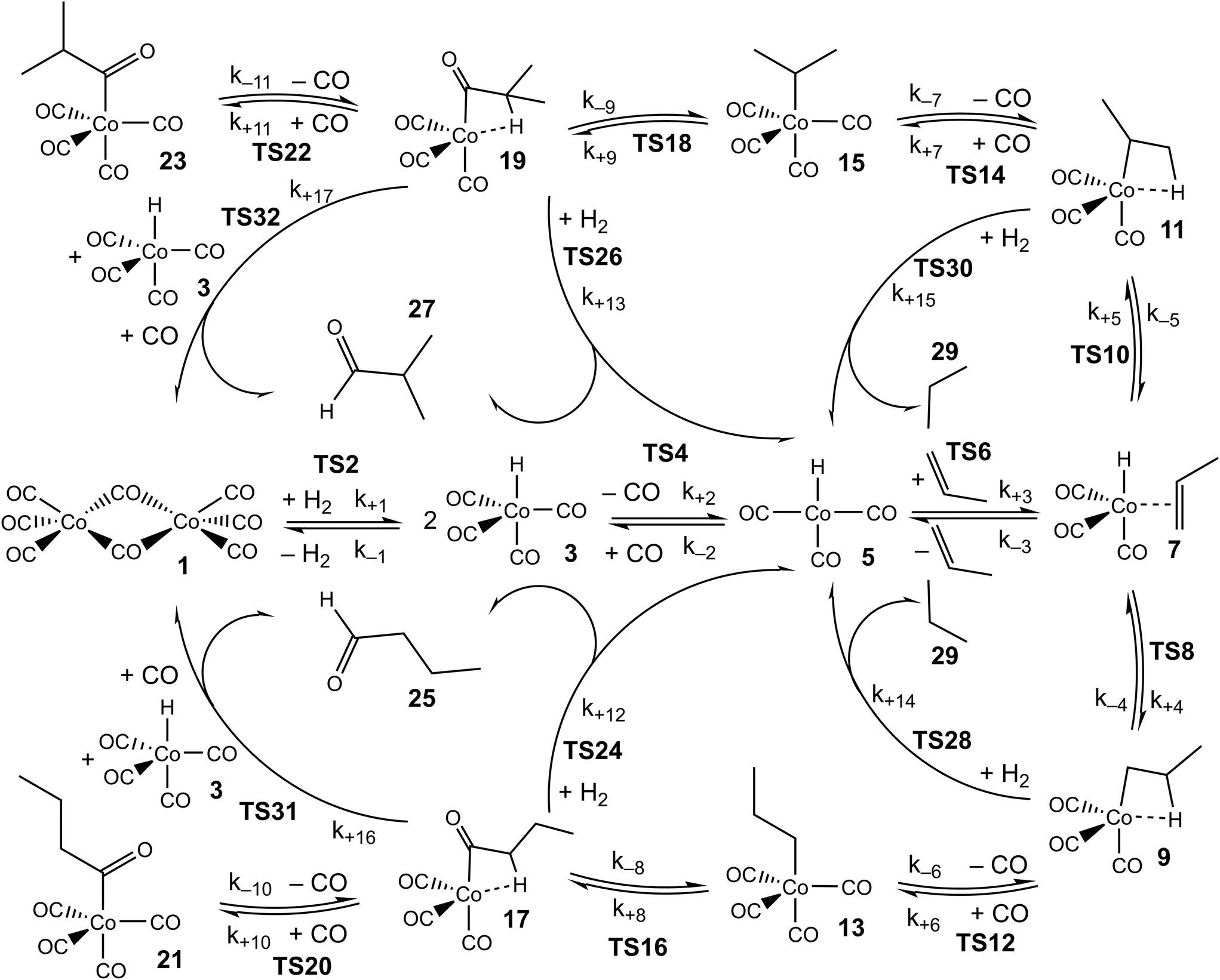 | ||
| Scheme 1 Reduced kinetic model for the mechanism of propene hydroformylation by Co2(CO)8. | ||
Then, at each temperature, the Gibbs energies for each species are obtained using ΔG = ΔH − TΔS, and Gibbs energies of activation are used together with the Eyring equation to calculate forward and reverse rate constants. For some reaction steps, typically ligand addition to coordinatively unsaturated cobalt complexes, for which no potential energy barrier occurs, the rate constant is computed not from ab initio Gibbs energies for the TS, but instead from a simple equation for rate constants of diffusion-limited reactions, with as parameters the solvent viscosity and the temperature.24 These values are obtained at the three temperatures mentioned above, then the Eyring equation is inverted to yield an ‘activation Gibbs energy’, and in the same way as above, a linear fit of these Gibbs energies provides standard values of the enthalpy and entropy of the associated barrierless transition states. For these steps, the rate constants for the reverse reactions are obtained from the rate constants for the forward reactions, the statistical mechanics-predicted equilibrium constants, and detailed balance. A further comment needs to be made concerning the steps leading to formation of butyraldehyde or propane, involving TSs 24, 26, 28, 30, 31, 32 in Scheme 1. In principle, these steps are reversible, and indeed some synthetic applications make use of reverse hydroformylation.46,47 Based on the ab initio free energies for n- and iso-butyraldehyde, propene, H2 and CO (see ESI†), and on the various experimental pressures of CO and H2 used in the reaction,25,26 the lowest predicted ratio of the equilibrium concentrations of n-butyraldehyde and propene is larger than 100, making the reaction essentially irreversible. For this reason, and for convenience in the modelling, we treat these reactions as being irreversible, i.e. we set the reverse rate constants to zero.
Based on the whole set of rate constants, the kinetic equations are propagated, holding the partial pressures of CO and H2 and the concentration of propene fixed, until steady-state is reached (the experimental measurements were carried out at steady-state; the partial pressures of CO and H2 and the concentration of propene were in large excess so were effectively constant). The resulting predicted rates for formation of the two main products, linear n-butyraldehyde and the branched isomer iso-butyraldehyde are then obtained, and can be compared directly to experimentally observed rates under a range of different experimental conditions (including variation of the temperature, the concentrations of catalyst and of propene, and the partial pressures of reagents H2 and CO).
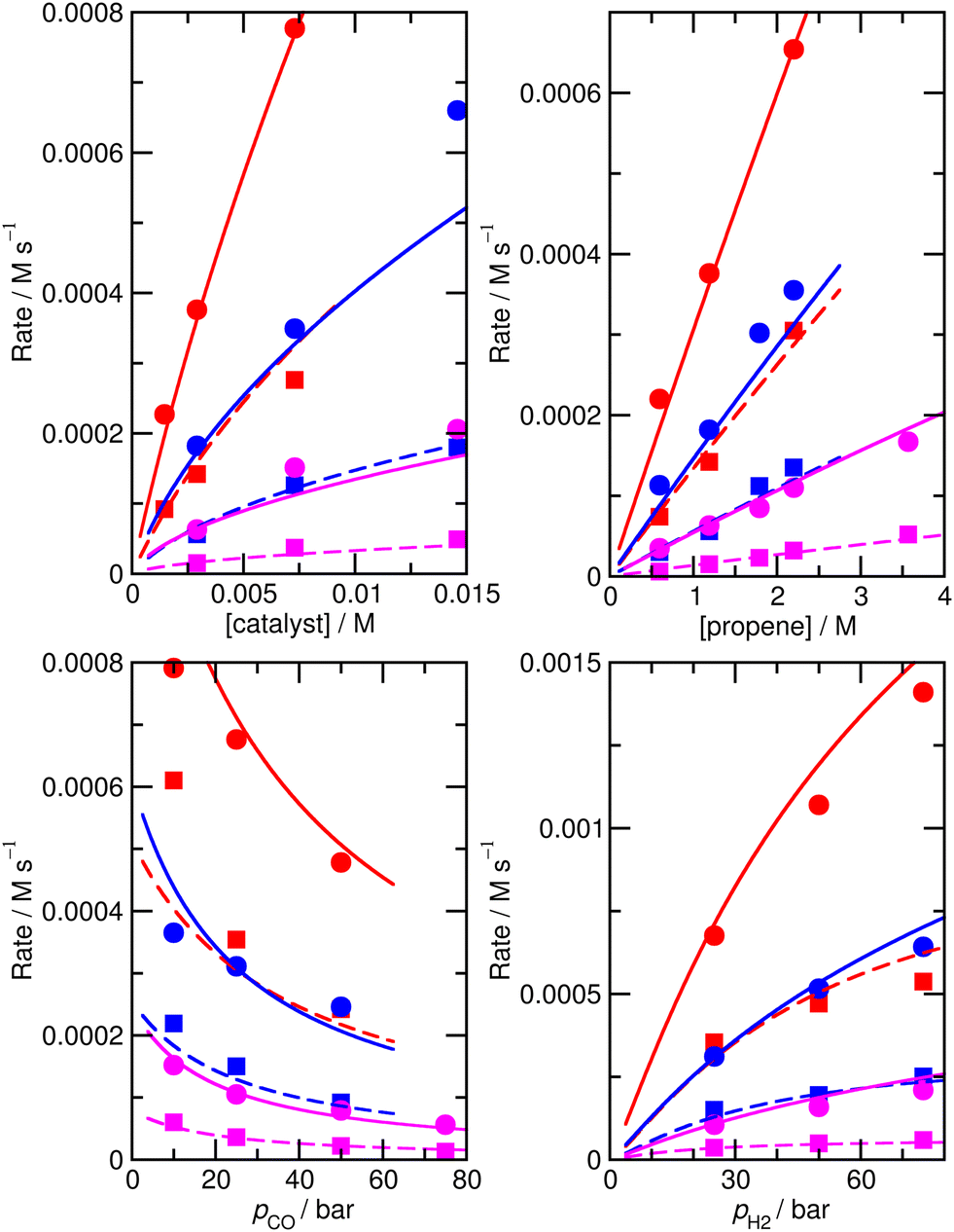
The accuracy of the kinetic model can be assessed in a number of ways; for the purposes of this study, we find that the most useful metric is the root mean-square (RMS) error χ of the predicted rates (or more precisely of the ratio of the calculated and observed rates,  where the sum runs over the N different experimental conditions, and Ri,pred and Ri,exp correspond to the predicted and experimental rates under those conditions) under the different experimental conditions, as used before,24 though we also consider two other metrics: the first of these is the maximum deviation between predicted and experimental rates, taken as the absolute value of the natural logarithm of the ratio Rpred/Rexp, i.e. |ln(Rpred/Rexp)|. A value of 1 for this metric indicates that one of the predicted rates differs from experiment by a factor 2.72 (either too large or too small). The second new metric is qualitative: the agreement of the shape of the curve of predicted rates as a function of the different variables with that observed experimentally. Following assessment of the zero-th order model, modified models are generated by changing the zero-th order enthalpies and entropies of the different species and transition states, and seeking to minimize the RMS error. These changes are performed using various constraints, as described below. Finally, where a large mismatch between the raw enthalpy or entropy and the fitted value is obtained, the quantum chemical calculated values are reinvestigated. The starting point is the same zero-th order model as used before,24 which we refer to here as model ‘M0’ (Table S1†), and which leads to an RMS error on predicted rates of 67.9%. This represents rather high accuracy considering that the rate constants are based on ‘raw’ unadjusted quantum chemical values, and remembering that at 150 °C, an error in Gibbs energy of 2.5 kJ mol−1 is sufficient to cause a change in a rate constant or equilibrium constant by a factor of 2, so the average agreement on rate with mean errors of ±67.9% suggests that our ab initio protocol for the key steps delivers an average accuracy of this order of magnitude. Still, the model does include some qualitative errors, notably for the dependence of the rate on temperature and on partial pressure of CO (Fig. 1). Also, the metric |ln(Rpred/Rexp)|max is quite large, at 2.75, indicating that one of the rates is incorrect by a factor exp(2.75) or about 15.6 – which suggests that at least one of the Gibbs energies in the model is wrong by almost 10 kJ mol−1. Therefore, we aim to improve our kinetic model by carrying out modifications of the ‘raw’ ab initio data. Instead of varying the calculated temperature-dependent ΔG values, we choose to instead vary the T-independent ΔH and ΔS values described above, as this guarantees that our fitted models are physically plausible in terms of the underlying ΔG values and their temperature dependence. We vary the “raw” enthalpies and entropies of the different species and transition states, while seeking to minimize the RMS error. In our earlier study,24 tight constraints were used with a maximum change of ab initio enthalpy and entropy values of 4 kJ mol−1 and 0.035 kJ mol−1 K−1. The maximum entropy change is equivalent to a change in Gibbs energy of 13–15 kJ mol−1 for the temperatures of 383–423 K modelled here. The modesty of the allowed changes was motivated by the high accuracy of CCSD(T) and of the initial M0 kinetic model, with the entropies considered to be more uncertain. Fitting with these allowed changes led to a best fit RMS error of 22%.24 Here, we repeated the fitting by allowing enthalpies and entropies for the same species 1, TS2, TS4, TS6, TS12, TS14, TS31, TS32 (species whose values have a higher uncertainty due to there being no CCSD(T) energies available or due to uncertainty in assigning rate constants for diffusion-limited reactions) to change, but with a more balanced maximum change of ab initio enthalpy and entropy values of 6 kJ mol−1 and 0.02 kJ mol−1 K−1. The maximum entropy change is equivalent to a change in Gibbs energy of around 8 kJ mol−1 for the temperatures of 383–423 K. In this fitting, we performed very thorough Monte-Carlo exploration of the space of H and S values in order to check that the optimum parameters had been found. This yields a best-fit RMS error of 22.9%, similar to the earlier result.24 The fitted ΔH, ΔS, and ΔG values and change with respect to ab initio values for this M1 model can be found in ESI† (Table S2). As in the previous study, this model yields much improved agreement with experiment particularly with regard to the dependence of rate on temperature (Fig. S1†). However, qualitatively, as for the fitted model in the previous study,24 this model still shows a significant error related to the predicted rate dependence for product formation on the partial pressure of CO. Also, |ln(Rpred/Rexp)|max remains quite large at 1.00.
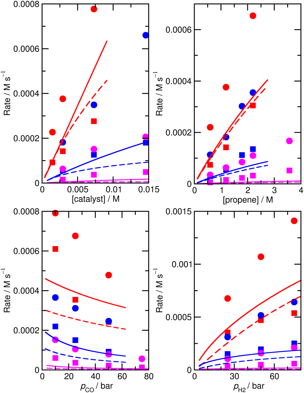 | ||
| Fig. 1 Predicted (lines) and experimental (points) rates for formation of n-butyraldehyde and iso-butyraldehyde under a range of different experimental conditions for M0. Experimental conditions: top left: pCO = pH2 = 50 bar, [propene] = 1.19 M; top right: pCO = pH2 = 50 bar, [catalyst] = 0.00292 M; bottom left: pH2 = 25 bar, [catalyst] = 0.0073 M, [propene] = 1.19 M; bottom right: pCO = 25 bar, [catalyst] = 0.0073 M, [propene] = 1.19 M. Red, 423 K; blue, 403 K; magenta, 383 K. Experimental rates for formation of n-butyraldehyde are shown as circles, and for iso-butyraldehyde as squares. Calculated rates for formation of n-butyraldehyde are shown as solid lines, and for iso-butyraldehyde as dashed lines. | ||
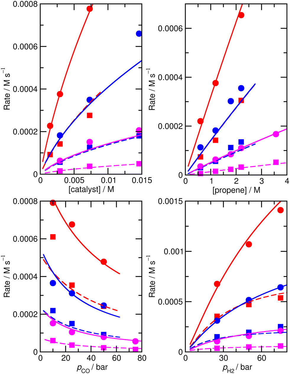
To check that the species for which ΔH and ΔS had been varied were indeed the key species, we then calculated the derivative of the RMS error with respect to ΔH and ΔS for all species for the initial, unfitted set of enthalpies and entropies i.e. for model M0, ∂χ/∂ΔH and ∂χ/∂(TΔS) (Table S3†). Both metrics yield similar info, so we used only ∂χ/∂ΔH to identify ‘important’ species (those where this metric is larger than 0.001, plus any n or iso counterpart where applicable). These species are 1, TS4, TS6, TS12, 13, TS14, 15, TS24, TS26, TS31, TS32. Then we again performed very thorough Monte-Carlo fitting by allowing these species to change and with a maximum change of ab initio enthalpy and entropy values of 6 kJ mol−1 and 0.02 kJ mol−1 K−1. This yields a best-fit model M2 (Table S4†) with a RMS error of 21.1%, slightly improved over M1, but the predicted rate dependence on the partial pressure of CO is not improved at all and |ln(Rpred/Rexp)|max remains quite large at 1.03 (Fig. 2).
 | ||
| Fig. 2 Predicted (lines) and experimental (points) rates for formation of n-butyraldehyde and iso-butyraldehyde under a range of different experimental conditions for M2. See Fig. 1 for full reaction conditions. | ||
These additional Monte-Carlo fittings confirm that a qualitatively accurate model (defined as having low RMS error, low maximum error, and correct dependence of rate on all experimental variables) cannot be found while maintaining Gibbs energies that match those obtained from the ab initio calculations within tight constraints. Therefore, we examined what would occur if we completely removed all constraints on the calculated enthalpy and entropy. Initially, this was done intuitively and by trial and error by carrying out a series of unconstrained Monte-Carlo fittings, leading as expected to major changes in ΔH and ΔS for many species and to unphysical relative Gibbs energy values and rate constants. As well as using Monte Carlo search, we also implemented an unconstrained gradient-based minimization algorithm to minimize the RMS error from the raw ab initio values in order to obtain more accurate location of minima, with the enthalpy and entropy values for all the species being allowed to vary. This led to a new model, ‘M3’ (Fig. S2, Table S5†), with a much lower RMS error of 10.2%, excellent dependence on CO partial pressure, and |ln(Rpred/Rexp)|max decreased to 0.29 (a maximum error by a factor of 1.3). An RMS error of the order of 10% starts to approach the type of accuracy that might be expected from the experimental study itself. Indeed, in the experimental study,25,26 a two-parameter empirical rate law was fitted to the experimental data, with separate fits at each of the temperatures, and this fit yielded agreement within 7%, so a fit achieving errors around 10% while relying on a first-principles model with a unique set of parameters for all temperatures probably represents something quite close to the maximum accuracy that can be expected.
The parameters in M3 include major changes in ΔH and ΔS and relative Gibbs energies for many species, leading to values that are in some cases unphysical (Table S5†). Clearly, the unconstrained fit of M3 is unrealistic in terms of the underlying elementary rate constants. Nevertheless, the significant improvement in the quality of the fit discussed above does suggest that M3, despite the unphysical values of some of the individual rate constants, may nevertheless capture the correct behavior of the whole kinetics for the right reasons in the broad sense.
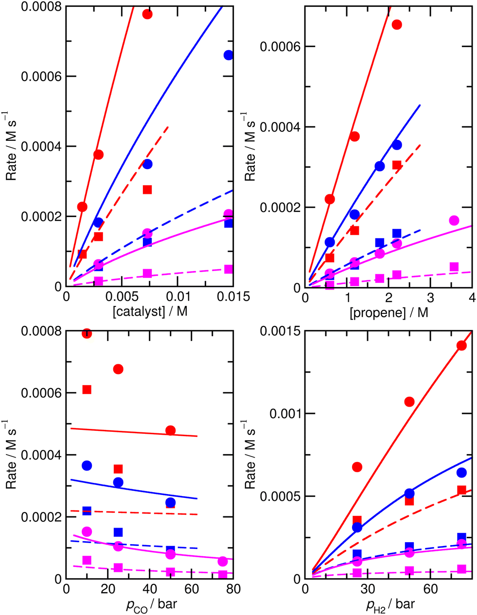
For this reason, we decided to investigate if nearly equivalent results could be obtained by carrying out partially unconstrained gradient-based minimization from the raw ab initio values, where we only allowed a small subset of enthalpies and entropies, which impact most significantly on the modelled rates, to vary without constraints but kept the values for other less important species fixed. Again, we use the absolute value of ∂χ/∂ΔH as a criterion for importance, retaining species where this metric exceeds 0.01, plus any n/iso counterpart, yielding species 1, TS4, TS6, TS24, TS26. Optimization of these yields model M4 (Fig. 3 and Table 1), still with a low RMS error of 13.4%, and |ln(Rpred/Rexp)|max of 0.41 (a maximum error by a factor of 1.5). This model again yields a qualitatively essentially correct dependence on the partial pressure of CO.
 | ||
| Fig. 3 Predicted (lines) and experimental (points) rates for formation of n-butyraldehyde and iso-butyraldehyde under a range of different experimental conditions for M4. See Fig. 1 for full reaction conditions. | ||
| Species | ΔH (fitted and change) | ΔS (fitted and change) | ΔG (fitted and change) | |||
|---|---|---|---|---|---|---|
| 1 | −95.9 | −77.9 | −0.167 | −0.178 | −32.0 | −9.9 |
| TS4 | 141.5 | −9.1 | 0.161 | 0.064 | 79.8 | −33.7 |
| TS6 | 35.5 | −118.5 | −0.148 | −0.282 | 92.2 | −10.4 |
| TS24 | 5.8 | −11.9 | −0.273 | −0.015 | 110.4 | −6.2 |
| TS26 | −0.7 | −11.7 | −0.285 | −0.022 | 108.4 | −3.4 |
Table 1 shows that the properties of TS6, the TS for addition of propene to HCo(CO)3, undergoes substantial changes in ΔH and ΔS upon fitting, with the enthalpy and entropy going down by 118.5 kJ mol−1 and 0.282 kJ mol−1 K−1, respectively. These changes partly cancel out in the resulting Gibbs energies, which thereby changes relatively little, with ΔG only decreasing by 10.4 kJ mol−1 at 383 K.
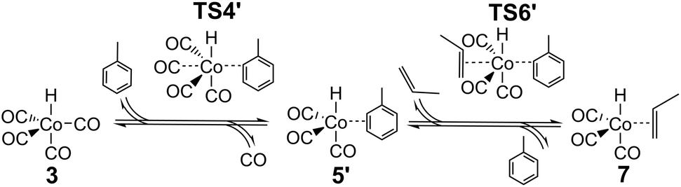
The major change in properties for TS6 suggest to us that the ab initio values for TS6 might be qualitatively wrong, perhaps due to incorrect description of solvation. As already shown,24 HCo(CO)3 can exist not only as an unsaturated free species under reaction conditions, but also as a complex with solvent if the latter is reasonably coordinating, as is the case for the toluene used in the experimental studies.25,26 If this complex is indeed formed under reaction conditions, then the reaction leading from HCo(CO)43 to HCo(CO)3(propene) 7 could proceed not dissociatively, but stepwise through concerted displacements (SN2-like) with intermediate formation of HCo(CO)3(toluene), where a CO ligand from HCo(CO)4 is first replaced by toluene to form HCo(CO)3(toluene) (TS4′), with a second step involving substitution of toluene by propene (TS6′) to form HCo(CO)3(propene) (Scheme 2).
 | ||
| Scheme 2 Proposed associative substitution mechanism for propene hydroformylation by Co2(CO)8. | ||
The complex and the two concerted associative TSs were then explored in new DFT calculations, including one explicit toluene solvent molecule (Table 2). The toluene complex 5′ is significantly lower in energy than HCo(CO)35 + toluene by 65.5 kJ mol−1, and importantly, the calculated Gibbs energy for 5′ is also lower than that of the fragments, by 15.8 kJ mol−1 at 383 K, supporting the idea that HCo(CO)3(toluene) 5′ is favored over 5 under reaction conditions. The calculated relative energies for TS4′ and TS6′ are also low, and similar to the experimental suggested activation energy of 77 kJ mol−1,25,26 as would be expected if the latter is close to the difference in energy between reactants and the bottleneck to reaction. The new Gibbs energies for TS4′ and TS6′ are similar to the old ones for TS4 and TS6. Note that canonical CCSD(T)-F12 values are not possible for these new species.
| Species | ΔE | ΔG |
|---|---|---|
| HCo(CO)43 + toluene + propene | 0.0 | 0.0 |
| TS4′ + propene | 67.7 | 105.1 |
| HCo(CO)3(toluene) 5′ + CO + propene | 60.8 | 53.4 |
| TS6′ + CO | 57.6 | 95.1 |
| 7 + CO + toluene | 30.1 | 29.1 |
| HCo(CO)35 + toluene + CO + propene | 126.3 | 69.2 |
As before, a linear fit of the ab initio Gibbs energies at different temperatures for TS4′, 5′ and TS6′ was carried out to obtain new ab initio enthalpies and entropies for these species, which can be compared to the initial ab initio enthalpies and entropies for TS4, 5 and TS6 (Table 3). The new enthalpies and entropies are all significantly lower than the old ones, while the Gibbs energies change much more modestly. The ΔH and ΔS values for TS6′ are also closer to the corresponding values in M4 (35.5 kJ mol−1 and −0.148 kJ mol−1 K−1). These results suggest that the concerted associative mechanism is more favorable than the dissociative mechanism. Taking these ‘new’ ab initio enthalpies and entropies for TS4′, 5′ and TS6′ together with the standard ab initio values for all other points, and modelling the kinetics, we get a ‘new’ ab initio model, which we refer to here as model MN, which has an RMS error on predicted rates of 34.9% and with |ln(Rpred/Rexp)|max quite large, at 0.93. The dependence of the rate on temperature is reasonable, and so is the predicted dependence of the rate on partial pressure of CO (Fig. S3†).
| Species | ΔH | ΔS | ΔG | ΔH | ΔS | ΔG |
|---|---|---|---|---|---|---|
| X = nothing | X = toluene | |||||
| TS: HCo(CO)4 → HCo(CO)3[X] | 150.6 | 0.097 | 113.5 | 74.5 | −0.080 | 105.1 |
| HCo(CO)3[X] | 144.7 | 0.156 | 84.9 | 66.8 | 0.035 | 53.4 |
| TS: HCo(CO)3[X] → HCo(CO)3(propene) | 154.0 | 0.134 | 102.5 | 69.3 | −0.068 | 95.1 |
Again, we decided to carry out fitting to improve the kinetic model, allowing species for which ∂χ/∂ΔH exceeds 0.001 (and their n/iso counterparts, see Table S6† for a full list of ∂χ/∂ΔH and ∂χ/∂TΔS for the ‘new’ ab initio model) i.e. species 1, TS4′, TS6′, TS12, 13, TS14, 15, TS24, TS26, TS31, TS32 to have modified enthalpy and entropy values. Fitting was performed using a Monte-Carlo approach with a maximum change of ΔH and ΔS values of 6 kJ mol−1 and 0.02 kJ mol−1 K−1, except for TS4′ and TS6′, where a larger maximum change of respectively 20 kJ mol−1 and 0.06 kJ mol−1 K−1 was allowed as the ab initio values are obtained with DFT and have a higher uncertainty. This yields M5 (Fig. 4 and Table S7†) with an excellent RMS error of 13.4%, very good dependence of rate on CO partial pressure, and a small |ln(Rpred/Rexp)|max of 0.37 (a maximum error by a factor of 1.4).
 | ||
| Fig. 4 Predicted (lines) and experimental (points) rates for formation of n-butyraldehyde and iso-butyraldehyde under a range of different experimental conditions for M5. See Fig. 1 for full reaction conditions. | ||
The largest remaining errors in this model are at the lowest CO partial pressure of 10 bar at the highest temperature, 423 K, where the predicted rate for formation of iso-butyraldehyde is smaller than experiment by 1.9 × 10⁻⁴ M s−1. Nevertheless, M5 provides an accurate model of the experimental rates, and suggests that the reaction mechanism indeed involves formation of a toluene complex of HCo(CO)3.
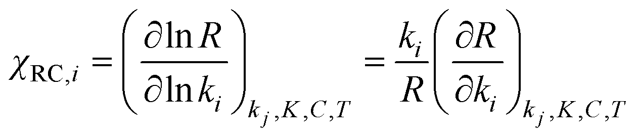
Assuming that M5 is very close to the correct kinetic model, we can address the question of which step is rate-limiting. Some indication can be found by referring to the values of ∂χ/∂ΔH in Table S6,† as large values of this quantity correspond to species whose thermodynamic properties impact most significantly on the modelled rates. However, a more powerful way to analyze this question is to use the degree of rate control (DRC) metric33,48 for the individual elementary steps, χRC,i. This is defined as the derivative of the logarithm of the rate R with respect to the logarithm of the rate constant for a given step, with all equilibrium constants and rate constants for other steps and the reaction conditions (e.g. the concentrations C of the reactants and the temperature T) held constant, eqn (1). In case the step i is reversible, i.e. in case the inverse rate constant k−i is non-zero, then the derivative is taken while holding the equilibrium constant for that step constant. In practice, to compute χRC,i, the kinetic model is integrated to obtain a predicted turnover rate R, then a given rate constant is multiplied by a small factor, and the model recomputed, and the numerical derivative is evaluated. For reversible steps, both ki and k−i are scaled by the same factor. A value of χRC,i = 0 for a given step indicates that this step is completely unimportant for determining the rate of turnover, while χRC,i = 1 indicates that the given step is the only one that is turnover-limiting, with intermediate values indicating partial control (in that case, the sum of the χRC,i for all steps will equal 1).
 | (1) |
| Reactions | DRCtotal | DRCn | DRCiso |
|---|---|---|---|
| Step 3 | 0.65 | 0.65 | 0.65 |
| Step 6 | 0.04 | 0.10 | −0.09 |
| Step 7 | 0.04 | −0.10 | 0.37 |
| Step 12 | 0.20 | 0.44 | −0.36 |
| Step 13 | 0.06 | −0.09 | 0.41 |
| Step 16 | 0.00 | 0.01 | −0.01 |
| Step 17 | 0.00 | 0.00 | 0.01 |
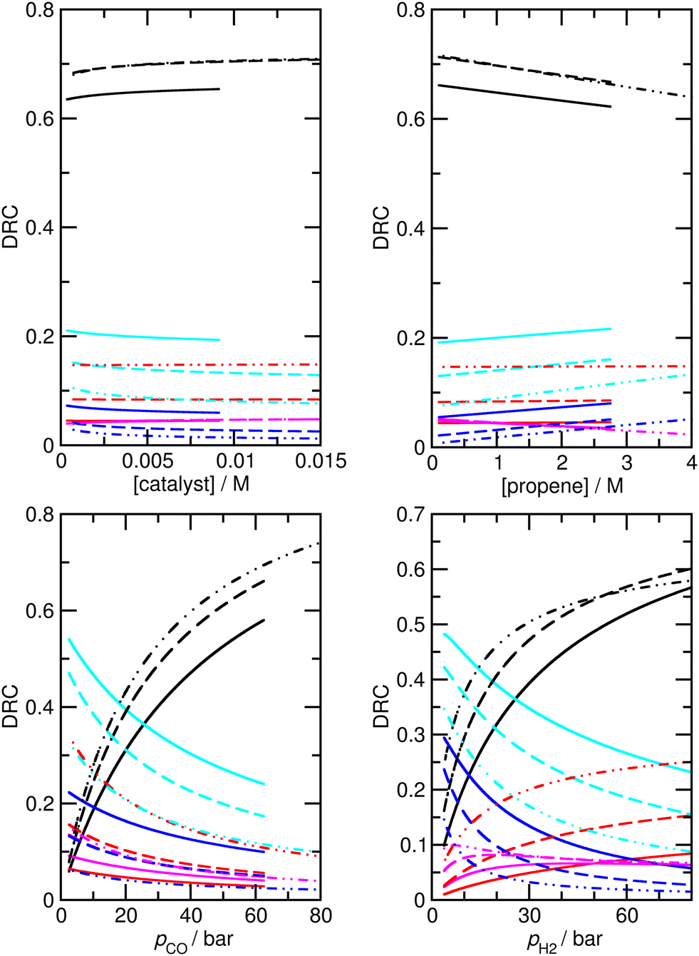 | ||
| Fig. 5 Calculated degree of rate control (DRC) values for formation of overall butyraldehyde products for M5 under a range of different experimental conditions. Experimental conditions: top left: pCO = pH2 = 50 bar, [propene] = 1.19 M; top right: pCO = pH2 = 50 bar, [catalyst] = 0.00292 M; bottom left: pH2 = 25 bar, [catalyst] = 0.0073 M, [propene] = 1.19 M; bottom right: pCO = 25 bar, [catalyst] = 0.0073 M, [propene] = 1.19 M. Black, step 3; red, step 6; magenta, step 7; cyan, step 12; blue, step 13; solid lines, 423 K; dashed lines, 403 K; dash double-dotted lines, 383 K. | ||
We find that under many conditions, more than one step exerts an influence on the rate, with the magnitude of χRC,i for different steps depending quite strongly on the reaction conditions. Under many conditions, the largest degree of rate control is associated with step 3 in Scheme 1, i.e. the addition of propene to HCo(CO)3, which in model M5 actually corresponds to substitution of toluene by propene in HCo(CO)3(toluene). Under the ‘most typical’ reaction conditions (T = 423 K, pCO = pH2 = 50 bar, [propene] = 1.19 M, and [catalyst] = 7.3 × 10⁻³ M), χRC for this step is 0.65 (whichever rate is used to compute χRC, i.e. the total rate of butyraldehyde formation, or those for n- or iso-formation, Table 4). While this large value indicates that propene addition has the dominant effect on turnover, the fact that it is significantly smaller than one indicates that other steps play a role also, in particular steps 6 and 7 (for addition of CO to RCo(CO)3, with R being n- or iso-propyl) and 12 and 13 (for H2-mediated cleavage of product from RCOCo(CO)3). Having multiple steps each partly determine turnover indicates a complex reaction mechanism, and carefully optimized reaction conditions, under which the optimal behavior of the individual steps is achieved.
Under different reaction conditions, the nature of the main turnover-limiting step can change. At low CO pressure, for example, step 12 (cleavage of the acyl–cobalt bond by hydrogen) becomes the dominant turnover-limiting step for formation of n-butyraldehyde (Fig. 5 and S4†). Changing the temperature also affects the contribution of the different steps to determining the rate of turnover. Under all conditions, though, multiple steps make non-negligible contributions. Overall, as already mentioned, the industrially most relevant experimental conditions with T near 400 K, and high pressures of CO and H2, can be seen to emerge as conditions where the optimum turnover rate is controlled by several steps.
Another important mechanistic question can be examined based on our accurate kinetic model M5, and this relates to the relative contributions of the reactions of H2 and HCo(CO)43 to the formation of butyraldehydes from the acyl–Co(CO)3 species 17 and 19, respectively reactions 12 and 13 (H2) and 16 and 17 (HCo(CO)4). At low temperature, under stoichiometric conditions, 3 is known to be able to effect the cleavage of acyl–Co(CO)3, but the contribution under practical catalytic turnover conditions is less well known. Here we have computed the proportion of the rate of aldehyde formation corresponding to the bimetallic route compared to the total rate of formation for the different experimental conditions (Fig. S6†). As expected, this proportion increases upon increasing the total cobalt concentration, and decreases upon increasing the partial pressure of H2. It also varies slightly with temperature, with pCO and with the concentration of propene. In all cases, the proportion of product formed the bimetallic mechanism remains quite small, under 6%. This suggests that the alternative mechanism does not play an essential role. However, examination of the fitting procedure that yields M5 shows that the Monte Carlo search visits values of the set of enthalpies and entropies that yield comparably accurate kinetic models, but indicate a higher proportion of product formed through the bimetallic mechanism.
For this reason, an alternative approach to assess the importance of this alternative mechanism was used, whereby a new model, M6, was constructed, in the same way as M5, except that the bimetallic steps were simply removed. Starting from the ‘new’ ab initio model MN, reactions 16 and 17 were removed, and a new fit to experiment was performed. The enthalpies and entropies of species 1, TS4′, TS6′, TS12, 13, TS14, 15, TS24, TS26 were allowed to undergo changes, and fitting was performed using a Monte-Carlo approach with a maximum change of ΔH and ΔS values of 6 kJ mol−1 and 0.02 kJ mol−1 K−1. Model M6 (Fig. 6 and Table S8†) has an excellent RMS error of 13.4%, very good dependence of rate on CO partial pressure, and |ln(Rpred/Rexp)|max of 0.39 (a maximum error by a factor of 1.5). This model M6 is thereby almost identical in terms of accuracy profile to M5 where the alternative bimetallic mechanism is included, further suggesting that the alternative bimetallic mechanism does not play an important role under industrial turnover conditions.
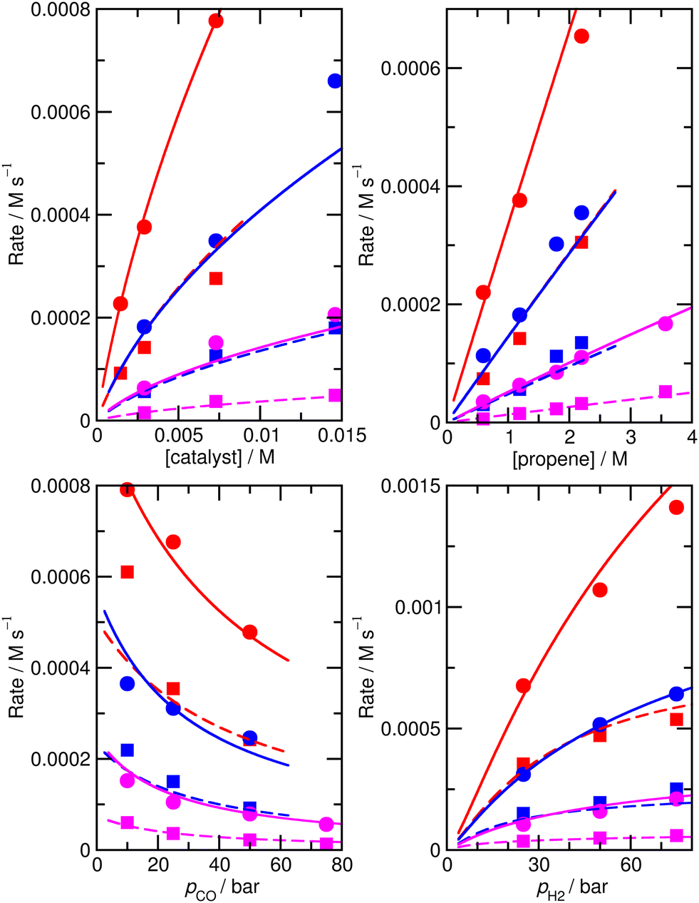 | ||
| Fig. 6 Predicted (lines) and experimental (points) rates for formation of n-butyraldehyde and iso-butyraldehyde under a range of different experimental conditions for M6. See Fig. 1 for full reaction conditions. | ||
Computational details
Quantum chemical calculations
All structures were optimized using the B3LYP49 density functional as implemented in Gaussian 16 rev. A03,50 using the Grimme dispersion correction with Becke–Johnson damping51 and the 6-311G(d) basis set52,53 on all atoms. Vibrational frequencies were computed at the same level of theory. Standard DFT integration grids were used throughout. For the Gibbs energy correction (computed at 383, 403 and 423 K), the rotational constants from the Gaussian 16 optimized structure were used together with the rigid rotor approximation, while the vibrational contribution was computed using the quasi-harmonic approximation,54 whereby vibrational frequencies with a magnitude smaller than a cut-off value of 50 cm−1 were replaced by frequencies of 50 cm−1 prior to computation of the harmonic oscillator thermal and entropic contributions. A standard state concentration of 1 M was used for all species, except for CO (an ideal gas standard state of 1 atm) and toluene, for computing the translational component. For toluene, we use as standard state the pure form of the liquid at the corresponding temperature (8.5, 8.2 and 8.0 M, respectively, at 383, 403 and 423 K).55Kinetic modeling and fitting
Two different approaches have been applied to minimize the RMS error between predicted and experimental rates with an in-house code, by carrying out modifications of the ab initio enthalpies and entropies of the different species and transition states. One is a constrained Monte-Carlo method, where random changes are made to the ab initio enthalpies and entropies but with maximum allowed changes for each species. Then Gibbs energies for each species were recalculated and used together with the Eyring equation to calculate forward and reverse rate constants, followed by integrating the kinetic equation until steady state to predict the rates for formation of products. If these modified enthalpies and entropies lead to a reduction in the RMS error, the update is accepted and the process iterates until a lowest RMS is found.Another method is gradient-based minimization by implementing the Broyden–Fletcher–Goldfarb–Shanno (BFGS) algorithm to minimize the RMS error. The derivative of the RMS error with respect to ΔH and ΔS for each species, ∂χ/∂ΔH and ∂χ/∂ΔS, are calculated numerically by re-propagating the kinetics with slightly modified ΔH and ΔS values. For this, we use a central difference approximation with step widths of 0.0001 kJ mol−1 for ΔH and 0.0001 J mol−1 K−1 for ΔS. The BFGS algorithm was then applied to seek a minimum of the RMS error with respect to ΔH and ΔS.
Conclusions
In summary, we explore the mechanism of propene hydroformylation by Co2(CO)8, using a combination of quantum-chemistry, kinetic modelling, and reference to experimental kinetics. We explore the origin of the remaining discrepancies between predicted and observed rates by carrying out systematic numerical fitting of the ‘raw’ ab initio kinetic model to the experiment, and propose this as a protocol for refined mechanism development in homogeneous catalysis. Initial attempts to obtain a high quality fit of the ‘raw’ ab initio model to the experimental kinetics while making only modest adjustments to the ab initio enthalpies and entropies of the key species were unsuccessful, but much improved agreement with experiment was obtained upon allowing some key species to undergo much larger adjustments of the ab initio enthalpy and entropy. This occurs in particular for the key transition state TS6 for addition of propene to HCo(CO)3, and has led us to suggest that the molecular representation of this TS in our previous models is qualitatively incorrect. If we assume that free HCo(CO)3 is not formed, being replaced in the mechanism by a solvated species HCo(CO)3(toluene), then TS6 is re-interpreted as a TS for exchange of toluene and propene.Based on this suggestion emerging from the kinetic fitting process, we re-examined the corresponding steps using quantum chemical methods, and we indeed could locate the HCo(CO)3(toluene) species and its TSs for exchange of toluene by CO or propene. The raw ab initio free energy for these species confirm that they could in principle compete with the coordinatively unsaturated HCo(CO)3 species. Kinetic modelling using the ab initio enthalpies and entropies computed for this new microscopic model led to acceptable agreement with experiment, but crucially, tightly constrained fitting using these new ab initio values as starting points led to a highly accurate model which surpasses previous models in terms of ability to reproduce experimental rate data and yields new microscopic insight into the mechanism.
Where enough high-quality experimental kinetics data is available, we suggest that this type of combined experimental, quantum-chemical and microkinetics modelling approach (possibly performed using a machine-learning automated protocol) can yield the highest level of insight available into microscopic reaction mechanisms in catalysis or elsewhere. Experiments are of course essential as purely computational techniques are not routinely able to provide quantitative results. Quantum chemistry is essential in order to provide detailed microscopic models. Kinetic simulations provide a bridge between the two approaches, and the synergy between all three techniques can lead to refinement of the models put forward based on only some of the approaches. A suggested flowchart for modelling complex reaction mechanisms with this approach is shown in Scheme S1.†
Catalysis of hydroformylation by cobalt carbonyl complexes is shown to follow a complex mechanism, with the coordination of propene to the cobalt center shown to be the main turnover-limiting step, but several other steps are also partly turnover-limiting, with the role of each step in determining catalytic rate depending in part on the reaction conditions.
Author contributions
LG performed all quantum-chemical and microkinetic studies, and together with JNH, conceptualized the problem, wrote the code for microkinetic model fitting, analyzed the data, and wrote the manuscript.Conflicts of interest
There are no conflicts to declare.Acknowledgements
L. G. appreciates the China Scholarship Council (CSC) for providing a doctoral scholarship (ref. CSC201906220183). The authors thank Dr. Ewa Szlapa for help with the toluene exchange TSs.References
- J. N. Harvey, F. Himo, F. Maseras and L. Perrin, ACS Catal., 2019, 9, 6803–6813 CrossRef CAS.
- A. S.-K. Tsang, I. A. Sanhueza and F. Schoenebeck, Chem. – Eur. J., 2014, 20, 16432–16441 CrossRef CAS PubMed.
- S. Santoro, M. Kalek, G. Huang and F. Himo, Acc. Chem. Res., 2016, 49, 1006–1018 CrossRef CAS PubMed.
- D. L. Davies, S. A. Macgregor and C. L. McMullin, Chem. Rev., 2017, 117, 8649–8709 CrossRef CAS PubMed.
- S. Ahn, M. Hong, M. Sundararajan, D. H. Ess and M.-H. Baik, Chem. Rev., 2019, 119, 6509–6560 CrossRef CAS PubMed.
- D. J. Durand and N. Fey, Acc. Chem. Res., 2021, 54, 837–848 CrossRef CAS PubMed.
- K. D. Vogiatzis, M. V. Polynski, J. K. Kirkland, J. Townsend, A. Hashemi, C. Liu and E. A. Pidko, Chem. Rev., 2019, 119, 2453–2523 CrossRef CAS PubMed.
- T. Sperger, I. A. Sanhueza, I. Kalvet and F. Schoenebeck, Chem. Rev., 2015, 115, 9532–9586 CrossRef CAS PubMed.
- W. M. C. Sameera and F. Maseras, WIREs Comput. Mol. Sci., 2012, 2, 375–385 CrossRef CAS.
- B. Li, H. Xu, Y. Dang and K. N. Houk, J. Am. Chem. Soc., 2022, 144, 1971–1985 CrossRef CAS PubMed.
- T. Wititsuwannakul, M. B. Hall and J. A. Gladysz, J. Am. Chem. Soc., 2022, 144, 18672–18687 CrossRef CAS PubMed.
- W. Thiel, Angew. Chem., Int. Ed., 2014, 53, 8605–8613 CrossRef CAS PubMed.
- T. Bligaard, J. K. Nørskov, S. Dahl, J. Matthiesen, C. H. Christensen and J. Sehested, J. Catal., 2004, 224, 206–217 CrossRef CAS.
- B. W. J. Chen, L. Xu and M. Mavrikakis, Chem. Rev., 2021, 121, 1007–1048 CrossRef CAS PubMed.
- A. Bruix, J. T. Margraf, M. Andersen and K. Reuter, Nat. Catal., 2019, 2, 659–670 CrossRef CAS.
- M. Besora and F. Maseras, WIREs Comput. Mol. Sci., 2018, 8, e1372 CrossRef.
- M. Jaraíz, J. E. Rubio, L. Enríquez, R. Pinacho, J. L. López-Pérez and A. Lesarri, ACS Catal., 2019, 9, 4804–4809 CrossRef.
- A. C. Brezny and C. R. Landis, ACS Catal., 2019, 9, 2501–2513 CrossRef CAS.
- C. E. Kefalidis, M. Davi, P. M. Holstein, E. Clot and O. Baudoin, J. Org. Chem., 2014, 79, 11903–11910 CrossRef CAS PubMed.
- A. H. Motagamwala and J. A. Dumesic, Chem. Rev., 2021, 121, 1049–1076 CrossRef CAS PubMed.
- Y. Mao, H.-F. Wang and P. Hu, WIREs Comput. Mol. Sci., 2017, 7, e1321 CrossRef.
- S. Kozuch and S. Shaik, Acc. Chem. Res., 2011, 44, 101–110 CrossRef CAS PubMed.
- L. E. Rush, P. G. Pringle and J. N. Harvey, Angew. Chem., Int. Ed., 2014, 53, 8672–8676 CrossRef CAS PubMed.
- E. N. Szlapa and J. N. Harvey, Chem. – Eur. J., 2018, 24, 17096–17104 CrossRef CAS PubMed.
- R. V. Gholap, O. M. Kut and J. R. Bourne, Ind. Eng. Chem. Res., 1992, 31, 1597–1601 CrossRef CAS.
- R. V. Gholap, O. M. Kut and J. R. Bourne, Ind. Eng. Chem. Res., 1992, 31, 2446–2450 CrossRef CAS.
- M. Kalek and F. Himo, J. Am. Chem. Soc., 2017, 139, 10250–10266 CrossRef CAS PubMed.
- M. Jaraíz, L. Enríquez, R. Pinacho, J. E. Rubio, A. Lesarri and J. L. López-Pérez, J. Org. Chem., 2017, 82, 3760–3766 CrossRef PubMed.
- Z. Benedek, M. Papp, J. Oláh and T. Szilvási, ACS Catal., 2020, 10, 12555–12568 CrossRef CAS.
- Y. Yu, Y. Zhu, M. N. Bhagat, A. Raghuraman, K. F. Hirsekorn, J. M. Notestein, S. T. Nguyen and L. J. Broadbelt, ACS Catal., 2018, 8, 11119–11133 CrossRef CAS.
- L. A. Suàrez, Z. Culakova, D. Balcells, W. H. Bernskoetter, O. Eisenstein, K. I. Goldberg, N. Hazari, M. Tilset and A. Nova, ACS Catal., 2018, 8, 8751–8762 CrossRef.
- R. J. Rama, C. Maya, F. Molina, A. Nova and M. C. Nicasio, ACS Catal., 2023, 13, 3934–3948 CrossRef CAS PubMed.
- J. Heitkämper, J. Herrmann, M. Titze, S. M. Bauch, R. Peters and J. Kästner, ACS Catal., 2022, 12, 1497–1507 CrossRef.
- L. Legnani, A. Darù, A. X. Jones and D. G. Blackmond, J. Am. Chem. Soc., 2021, 143, 7852–7858 CrossRef CAS PubMed.
- J. Pham, C. E. Jarczyk, E. F. Reynolds, S. E. Kelly, T. Kim, T. He, J. M. Keith and A. R. Chianese, Chem. Sci., 2021, 12, 8477–8492 RSC.
- C. Goehry, M. Besora and F. Maseras, ACS Catal., 2015, 5, 2445–2451 CrossRef CAS.
- T. A. Young, J. J. Silcock, A. J. Sterling and F. Duarte, Angew. Chem., 2021, 60, 4266–4274 CrossRef CAS PubMed.
- P. Ramos-Sánchez, J. N. Harvey and J. A. Gámez, J. Comput. Chem., 2023, 44, 27–42 CrossRef PubMed.
- S. Maeda, K. Ohno and K. Morokuma, Phys. Chem. Chem. Phys., 2013, 15, 3683–3701 RSC.
- S. Habershon, J. Chem. Theory Comput., 2016, 12, 1786–1798 CrossRef CAS PubMed.
- J. Proppe and M. Reiher, J. Chem. Theory Comput., 2019, 15, 357–370 CrossRef CAS PubMed.
- J. Proppe, T. Husch, G. N. Simm and M. Reiher, Faraday Discuss., 2016, 195, 497–520 RSC.
- E. H. P. Tan, G. C. Lloyd-Jones, J. N. Harvey, A. J. J. Lennox and B. M. Mills, Angew. Chem., Int. Ed., 2011, 50, 9602–9606 CrossRef CAS PubMed.
- J. E. Sutton, W. Guo, M. A. Katsoulakis and D. G. Vlachos, Nat. Chem., 2016, 8, 331–337 CrossRef CAS PubMed.
- C. W. Gao, M. Liu and W. H. Green, Int. J. Chem. Kinet., 2020, 52, 266–282 CrossRef CAS.
- B. N. Bhawal and B. Morandi, Chem. – Eur. J., 2017, 23, 12004–12013 CrossRef CAS PubMed.
- S. K. Murphy, J.-W. Park, F. A. Cruz and V. M. Dong, Science, 2015, 347, 56–60 CrossRef CAS PubMed.
- C. T. Campbell, ACS Catal., 2017, 7, 2770–2779 CrossRef CAS.
- A. D. Becke, J. Chem. Phys., 1993, 98, 5648–5652 CrossRef CAS.
- M. J. Frisch, G. W. Trucks, H. B. Schlegel, G. E. Scuseria, M. A. Robb, J. R. Cheeseman, G. Scalmani, V. Barone, G. A. Petersson, H. Nakatsuji, X. Li, M. Caricato, A. V. Marenich, J. Bloino, B. G. Janesko, R. Gomperts, B. Mennucci, H. P. Hratchian, J. V. Ortiz, A. F. Izmaylov, J. L. Sonnenberg, D. Williams-Young, F. Ding, F. Lipparini, F. Egidi, J. Goings, B. Peng, A. Petrone, T. Henderson, D. Ranasinghe, V. G. Zakrzewski, J. Gao, N. Rega, G. Zheng, W. Liang, M. Hada, M. Ehara, K. Toyota, R. Fukuda, J. Hasegawa, M. Ishida, T. Nakajima, Y. Honda, O. Kitao, H. Nakai, T. Vreven, K. Throssell, J. A. Montgomery Jr. , J. E. Peralta, F. Ogliaro, M. J. Bearpark, J. J. Heyd, E. N. Brothers, K. N. Kudin, V. N. Staroverov, T. A. Keith, R. Kobayashi, J. Normand, K. Raghavachari, A. P. Rendell, J. C. Burant, S. S. Iyengar, J. Tomasi, M. Cossi, J. M. Millam, M. Klene, C. Adamo, R. Cammi, J. W. Ochterski, R. L. Martin, K. Morokuma, O. Farkas, J. B. Foresman and D. J. Fox, Gaussian 16, Revision A.03, Gaussian, Inc., Wallingford CT, 2016 Search PubMed.
- S. Grimme, S. Ehrlich and L. Goerigk, J. Comput. Chem., 2011, 32, 1456–1465 CrossRef CAS PubMed.
- R. Krishnan, J. S. Binkley, R. Seeger and J. A. Pople, J. Chem. Phys., 1980, 72, 650–654 CrossRef CAS.
- A. D. McLean and G. S. Chandler, J. Chem. Phys., 1980, 72, 5639–5648 CrossRef CAS.
- R. F. Ribeiro, A. V. Marenich, C. J. Cramer and D. G. Truhlar, J. Phys. Chem. B, 2011, 115, 14556–14562 CrossRef CAS PubMed.
- R. D. Goodwin, J. Phys. Chem. Ref. Data, 1989, 18, 1565–1636 CrossRef CAS.
Footnote |
| † Electronic supplementary information (ESI) available. See DOI: https://doi.org/10.1039/d3cy01625k |
| This journal is © The Royal Society of Chemistry 2024 |