Experimental and simulation study of reverse micelles formed by aerosol-OT and water in non-polar solvents

Abstract

The formation of reverse micelles by aerosol-OT [sodium bis(2-ethylhexyl) sulfosuccinate] in hydrocarbon solvents, and in the presence of water, is studied using a combination of atomistic molecular-dynamics simulations and small-angle neutron scattering (SANS). There have been many previous studies of aerosol-OT and its self-assembly in both water and non-aqueous solvents, but this work is focused on a combined experimental and simulation study of reverse-micelle formation. The effects of hydration (with water-to-surfactant molar ratios in the range 0–60) and solvent (cyclohexane and n-dodecane) are investigated. A force field is adapted that results in spontaneous formation of reverse micelles starting from completely randomized configurations. The computed dimensions of the reverse micelles compare very favourably with those determined in SANS experiments, providing validation of the simulation model. The kinetics of reverse-micelle formation are studied with a 50-ns, 1.7-million-atom system which contains, in the steady state, about 50 reverse micelles. The internal structures of reverse micelles are characterized with mass density profiles, and the effects of solvent, and the structural crossover from highly structured water to ‘bulk’ water in the core, are detailed. The corresponding changes in the molecular reorientation times of sequestered water are also determined. Overall, the combination of experiment and simulation gives a detailed picture of reverse-micelle self-assembly and structure.

---

1 Introduction

The molecule of interest in this study is sodium bis(2-ethylhexyl) sulfosuccinate, more commonly known as aerosol-OT (AOT).¹ It is a well-studied species defined by a sulfonate head group, and two aliphatic tails. (The molecular structure is given in the ESI.†) AOT is a versatile anionic surfactant with many applications ranging from medicinal² to industrial.³ AOT is notable for forming reverse micelles (RMs) in non-polar solvents.^4–8 Each RM consists of a polar core protected by the aliphatic tails which point outward into the solvent. The resulting small, polar pockets can solvate water, counterions, or other polar molecules present in an otherwise non-polar environment. The core can swell in order to accommodate increasing water content⁹ and serve as a suitable site for synthesis or catalysis, acting as a so-called ‘nanoreactor’.^10,11 An important parameter for RM formation in non-polar solvents is the hydration ratio (ω), being the molar ratio of water to surfactant. The water cores at lower hydration ratios (ω = 1–15) exhibit notably different behaviour to that of bulk water, as has been shown in various experimental studies.^12,13 AOT can also form normal micelles in aqueous solutions,¹⁴ but this is not the focus of this work.

One of the principal aims of the current study is to study the self-assembly of AOT RMs using atomistic molecular-dynamics (MD) simulations. While there are numerous computational studies available, the bulk of earlier modelling work uses fully or partially preassembled RMs in the investigated systems.^15–17 Some studies have been focused on the polar core of the RMs, with the non-polar portions and solvent represented by a single continuum.^18–23 Other work, more focused on RM shape and assembly, employed full or partial coarse-graining, especially for modelling the solvent.^24,25 While such studies offer important information, it is preferable to be able to treat all aspects of RM self-assembly with a fully atomistic model. To this end, Abel et al. developed all-atom models to simulate RM structures of AOT with water in isooctane,^15,16 which have been used subsequently to study the thermodynamics of RM formation.²⁶ Such models should also capture the self-assembly of RMs starting from random configuration, without constraints, and produce observable properties comparable to those measured in experiments. While there are experimental data already in the literature, primarily from small-angle neutron scattering (SANS) studies,^4,6–8 it is worth assessing MD predictions against new measurements.

The aims of the present work are to use MD simulations to study the self-assembly of AOT RMs both in pure (dry) solvents, and in the presence of water. To this end, new SANS experiments are carried out, and the effects of solvent are determined. The results of these experiments – along with those already in the literature^4,6–8 – are used to test a newly developed set of force-field parameters for MD modelling of AOT self-assembly. It should be noted, however, that the simulation work is not in any way parameterized from the experimental results; instead, the simulation predictions and experimental results are compared directly and critically. Novel microscopic details are revealed in the simulations, including the interior structure of the RM, the kinetics of RM self-assembly, and the reorientational dynamics of water molecules encapsulated within the RM. The results of this research will form the basis for ongoing studies of AOT adsorption from hydrocarbons onto inorganic surfaces, for various applications involving the modification of solid–liquid interfaces.

The rest of this article is organized as follows. The experimental and simulation procedures are described in Sections 2.1 and 2.2, respectively. The results are presented as follows: Section 3.1 – experimental results; Section 3.2 – comparisons between simulation and experimental results; Section 3.3 – the kinetics of RM self-assembly; Section 3.4 – the interior structure of the RMs; and Section 3.5 – the reorientational dynamics of water inside RMs. Section 4 concludes the article.

2 Materials, models, and methods

2.1 Experimental procedure

Sodium bis(2-ethylhexyl) sulfosuccinate (AOT, Sigma Aldrich, ≥97%), H₂O (Milli-Q water purifier, 18.2 MΩ cm), D₂O (Sigma Aldrich, 99.9% D), d₁₂-cyclohexane (Apollo Scientific, 99.5% D), and d₂₆-n-dodecane (Apollo Scientific, 98% D) were used as received from suppliers. SANS samples were prepared by mixing AOT in the relevant deuterated solvent, and adding D₂O or H₂O to the required values of ω = [water]/[AOT] and total volume. Samples were shaken vigorously until they appeared to be transparent and homogeneous.

The SANS experiments were carried out on the Sans2d instrument at ISIS Neutron and Muon Source (Didcot, UK), and the D33 instrument at Institut Laue-Langevin (Grenoble, France). Sans2d offers a Q range of 0.004–0.6 Å⁻¹, and wavelengths of neutrons in the range 1.75–15.5 Å. The source-sample-detector distances were set to L₁ = L₂ = 4 m, with the 1 m² detector offset vertically by 80 mm and sideways by 100 mm. D33 offers a Q range of 0.006–0.6 Å⁻¹, with a neutron wavelength of 4.6 Å, and one sample-detector distance of 8 m. The experiments were carried out at 25 °C using 2-mm rectangular quartz cells. The empty quartz cell and relevant solvent background scattering was subtracted from the raw SANS data, and reduced using software available at the instruments.

2.2 Molecular-dynamics simulations

MD simulations were carried out using LAMMPS.^27–29 The calculations were carried out in a cubic simulation cell with periodic boundary conditions applied in all directions (x, y, and z). The equations of motion were integrated using the velocity-Verlet algorithm.³⁰ The Nosé–Hoover thermostat/barostat was used to control the temperature and pressure;³⁰ the relaxation times were 0.1 ps and 1 ps, respectively.

The organic species were described with OPLS-type force fields^31–35 or variations thereof, as described below, with a real-space cut off of 12 Å. Standard all-atom and united-atom OPLS parameters can be accessed conveniently using online resources such as LigParGen^36–39 and Tinker (this work).^40,41 In the UA version, CH_n units are described as single interaction sites. Water was described with the TIP3P (Ewald) force field.⁴² In all simulations, the Lennard-Jones cross-interactions were calculated using the Berthelot mixing rule ³⁰ and Good-Hope mixing rule .⁴³ The long-range Coulombic interactions were handled using the particle–particle particle-mesh method with a real-space cut off of 12 Å and a relative accuracy in the forces of 10⁻⁴.

The OPLS force-field parameters required some tuning in order to reproduce spontaneous self-assembly of AOT. Initial tests with the united-atom, OPLS-UA force field failed to produce a self-assembled RM. As a result, an all-atom approach was selected for further work. The solvent (cyclohexane or n-dodecane) was described with the all-atom, L-OPLS-AA (or OPLS-AA/L) force field. Some clustering was observed in simulations using the L-OPLS-AA force field for AOT as well, but the comparison with then-available experimental results^4,6–8 was still poor. Assuming that the sulfonate head group on AOT was key, non-bonded OPLS-type parameters were taken from the force field for sodium dodecyl sulfate developed by Abdel-Azeim,⁴⁴ and this led to an improvement in the match with experimental results. However, there were still discrepancies and it became apparent that there was a need for bespoke partial charges for AOT. To this end, the partial charges on the head group in vacuo were determined from scratch by using density functional theory (DFT) calculations. Using the atom labelling scheme shown in Fig. S1 of the ESI,† the head group was represented by the fragment from C5 and H5 on one side chain to C5 and H5 on the other, terminated at each end with a methyl group. Geometry optimization calculations were carried out in Gaussian, with the B3LYP functional, 6-311++g(2d,2p) basis set, and a convergence criterion of 10⁻⁴ eV.⁴⁵ The sulfonate-group Lennard-Jones parameters (from ref. 44) and Mulliken partial charges on the head group (from this work) are given in the ESI.† All other parameters were from the L-OPLS-AA force field.

The system setup was geared toward observing self-assembly and determining aggregate properties, with the majority of simulations focused on self-assembly of a single RM. The various system compositions are detailed in Table 1, and contained between sixteen and sixty thousand atoms. To ensure a completely random initial configuration, the starting coordinates were generated using PACKMOL.^46,47 Each system was equilibrated first in the NVE ensemble for 1 ps with an integration time step of δt = 0.1 fs, then in the NVT ensemble at T = 298.15 K for 2 ns with δt = 0.5 fs, and lastly in the NPT ensemble at P = 1 atm and T = 298.15 K with δt = 1 fs for 2.5 to 5 ns. Production runs were then carried out in the NPT ensemble at P = 1 atm and T = 298.15 K with δt = 2 fs until the structure had ‘equilibrated’ in the sense defined below. This typically took place in 10s of nanoseconds.

Table 1 Compositions of the systems studied with MD simulations. N_AOT, N_H2O, and N_solvent are the numbers of AOT, water, and solvent molecules, respectively. ω is the hydration ratio, the molar ratio of water to AOT. N_agg is the AOT aggregation number of a micelle, and R_g is the radius of gyration of a micelle; R_g is determined either from a direct calculation (eqn (1)) or by fitting a simulated form factor (eqn (2) and (5)). Where the aggregation number is lower than the value of N_AOT, the R_g value is that of the largest RM in the system. The stated uncertainties are fitting errors, and rounded off to 2 decimal places

N AOT	N H2O	ω	Solvent	N solvent	N agg	R g(direct)/Å	R g[P(Q)]/Å
10	50	5	Cyclohexane	850	10	11.48 ± 0.01	11.59 ± 0.01
20	100	5	Cyclohexane	1700	20	13.87 ± 0.01	14.02 ± 0.01
40	200	5	Cyclohexane	3400	26	15.25 ± 0.01	15.55 ± 0.01
30	0	0	Cyclohexane	2600	13	11.65 ± 0.01	11.67 ± 0.01
30	30	1	Cyclohexane	2600	9	10.08 ± 0.01	10.14 ± 0.01
30	150	5	Cyclohexane	2600	14	12.96 ± 0.01	13.12 ± 0.01
30	300	10	Cyclohexane	2600	25	17.15 ± 0.05	16.80 ± 0.02
30	450	15	Cyclohexane	2600	30	18.64 ± 0.01	18.65 ± 0.01
30	1800	60	Cyclohexane	2600	30	24.92 ± 0.01	26.30 ± 0.10
30	0	0	n-Dodecane	1200	17	11.67 ± 0.01	11.75 ± 0.01
10	50	5	n-Dodecane	400	10	11.29 ± 0.01	11.40 ± 0.01
20	100	5	n-Dodecane	800	20	13.77 ± 0.01	13.99 ± 0.01
30	150	5	n-Dodecane	1200	30	14.79 ± 0.01	15.07 ± 0.01
40	200	5	n-Dodecane	1600	33	15.78 ± 0.01	16.13 ± 0.01

---

The single-RM studies were supplemented by a 50-ns simulation containing 1000 AOT molecules, 5000 water molecules, and 90 000 cyclohexane molecules at P = 1 atm and T = 298.15 K. There were about 1.7 million atoms in a box with length L = 259 Å. The AOT concentration equated to 95.6 mM. The aims of this study were to explore the kinetics of self-assembly, and determine whether the RM size was affected by such a high AOT concentration. The analysis of this simulation is described separately in Section 3.3.

The meaning of ‘equilibration’ here refers to the process of the simulation reaching a steady state, which is not necessarily the same as reaching thermodynamic equilibrium in a bulk system. Firstly, in a simulation of an isolated RM, once it has assembled there are no other processes that can take place, since there are no other molecules or RMs. Secondly, in real systems, there might be processes that lead to slow RM growth (such as Ostwald ripening) or even the formation of water-in-oil emulsions, but these are well beyond the (atomistic) simulation time scale. The saving grace is that on the experimental time scale of hours and beyond, RMs are apparently stable, and no emulsification is seen; the solutions remain transparent and homogeneous. Hence, while there is a large gap between simulation and experimental time scales, it is meaningful to compare the sizes of RMs formed in 10s of nanoseconds in simulations and RMs that exist for hours and longer in experiments. In short, ‘equilibration’ and ‘equilibrium’ are used here as shorthand for the simulations having reached a steady state because of either the limitation on system size (a single RM) or the limitation on time scale (many RMs).

A key parameter for the comparison between experiment and simulation is the radius of gyration R_g of a RM. In the MD simulations, this was obtained using a direct calculation, and by fitting a computed form factor. All calculations were carried out on distinct RMs, and any ‘excess’ molecules not part of the RM were removed. The direct calculation was made using the formula

where r_i is the position vector of atom i, and N is the total number of atoms in the RM (including any water). The separation vector was computed with the periodic boundary conditions unwrapped, so that it gives the true distance r_ij = |r_j − r_i| between atoms in the same RM, and not the minimum-image distance. The form factor P(Q) was computed using the formulawhere as before, the sums are restricted to all atoms in the same RM, and Q is the magnitude of the scattering wave vector Q. In SANS experiments, the scattered intensity is

I(Q) = P(Q)S(Q), (3)

where S(Q) is the structure factor describing spatial correlations between different RMs.⁴⁸P(Q) is usually fitted with a range of structural models, and the best one is assumed to reflect reality. The exact, low-Q behaviour of P(Q) is given by the Guinier approximationwhich is independent of the aggregate shape. An heuristic extension of this formula to larger wave vectors is the Gaussian formulawhich is also the form factor for a spherical object with a Gaussian scattering-length density profile.⁴⁹ The results from fitting P(Q) from experiments and simulations are compared to those from the direct calculation. The interior structure of a RM was investigated by calculating the radial mass-density profiles ρ(r) for atoms in each of the chemical components (AOT anion, Na⁺, water, solvent), where r is the radial distance from the centre of mass of the RM.

3 Results

3.1 Experimental results

New SANS data are shown in Fig. 1 for four cases: (a) 0.05 M AOT in cyclohexane, with hydration ratios ω = 5 and ω = 10; and (b) 0.05 M and 0.10 M AOT in dry d-dodecane. The data were first fitted using the Gaussian model (eqn (5)) plus a small background in the range Q ≤ 0.1 Å⁻¹, yielding the values given in the figure. For 0.05 M AOT in cyclohexane, the radius of gyration increases from R_g ≃ 15 Å to R_g ≃ 19 Å on increasing the hydration ratio from ω = 5 to ω = 10. This is due to the swelling effect of encapsulating water in the interior of the RM; the details of this mechanism will be discussed with reference to simulations in Section 3.4. In dry d-dodecane, the radius of gyration is R_g ≃ 12 Å and only weakly dependent on the AOT concentration.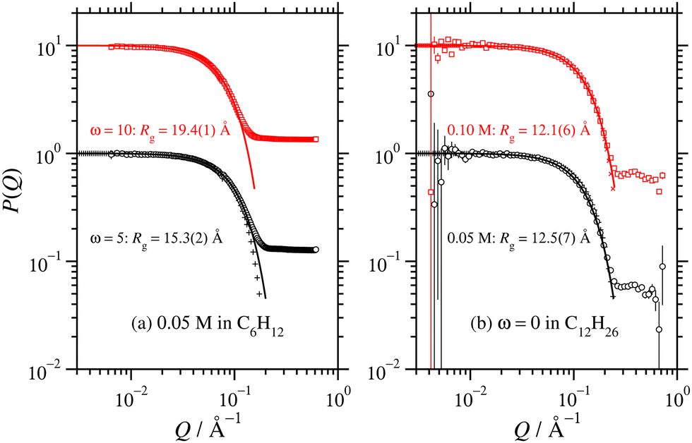

Fig. 1 Direct comparisons between the form factors from SANS experiments (circles and squares) and MD simulations (plusses and crosses): (a) 0.05 M AOT in cyclohexane with ω = 5 and 10 (SANS with H₂O and d-cyclohexane, MD with ω = 5 only and N_AOT = 40); (b) 0.05 M and 0.10 M AOT in dodecane with ω = 0 (SANS with D₂O and d-dodecane, MD with N_AOT = 30). The solid lines are fits of the Gaussian function (eqn (5)), plus a small background, to the SANS results in the range Q ≤ 0.1 Å⁻¹; the values of R_g shown are from these fits, and they are also given in Table 2. The fits to the MD results over the same Q range are omitted for clarity, but the parameters are given in Table 1. Data are scaled by ten units along the ordinate for clarity.

The SANS results are analyzed in a slightly different way in Fig. 2. Here, the shape-independent Guinier plot is used to check that the apparent radii of gyration are not strongly affected by the fitting method. The results are fitted using eqn (4) yielding values of R_g that deviate insignificantly from the values from the Gaussian fits.

Fig. 2 Direct comparisons of the form factors from SANS experiments (circles and squares) and MD simulations (plusses and crosses) in the form of Guinier plots: (a) 0.05 M AOT in cyclohexane with ω = 5 and 10 (SANS with H₂O and d-cyclohexane, MD with ω = 5 only and N_AOT = 40); (b) 0.05 M and 0.10 M AOT in dodecane with ω = 0 (SANS with D₂O and d-dodecane, MD with N_AOT = 30). The solid lines are fits of the Guinier law (eqn (4)), plus a small background, to the SANS results in the range Q² ≤ 0.004 Å⁻²; the values of R_g shown are from these fits, and they are also given in Table 2. The dashed lines are the corresponding Guinier plots with the radii of gyration computed directly from MD simulations (given in Table 1). Data sets are shifted by one unit along the ordinate for clarity.

Table 2 Radii of gyration from fitting the Gaussian model eqn (5)) and the Guinier approximation (eqn (4)) to new SANS data

c AOT/M	Solvent	ω	R g/Å (eqn (5))	R g/Å (eqn (4))
0.05	d-Cyclohexane	5	15.25 ± 0.25	15.05 ± 0.05
0.05	d-Cyclohexane	10	19.42 ± 0.15	18.56 ± 0.04
0.05	d-Dodecane	0	12.54 ± 0.75	12.07 ± 0.17
0.10	d-Dodecane	0	12.15 ± 0.64	12.03 ± 0.13

---

All of the values from fitting the experimental SANS data are collected in Table 2. This shows that the apparent radii of gyration agree within 1 Å, and are therefore reliable. Both Fig. 1 and 2 include simulation results, which are discussed in Section 3.2. A similar analysis on previously published SANS data gives comparable results.^4,6–8

3.2 Development and assessment of force-field parameters against experimental data

Despite many previous studies of AOT and its self-assembled structures, the simulation of spontaneous RM formation has not proven straightforward. The aim here was to start a simulation from a completely disordered configuration, and generate a self-assembled structure without external influence or constraints. In preliminary tests, simulations with off-the-shelf force fields, including all-atom and united-atom varieties, led either to small clusters or trivial phase-separated solute droplets. Given that all-atom force fields for the solvent, water, and surfactant tails are generally quite reliable, attention was focused on the description of the polar head group. Due to the scarcity of suitable charge parameters for the sulfonate head group, a DFT calculation was carried out with the B3LYP hybrid functional and 6-311++g(2d,2p) basis set.⁴⁵ The resulting partial charges were combined with literature values for the Lennard-Jones parameters,⁴⁴ as detailed in Section 2.2 and the ESI.† With these parameters, spontaneous self-assembly of an RM could be observed on the time scale of tens of nanoseconds. The general procedure was to choose a hydration ratio, and then add solute molecules until RMs were formed. An estimate of the aggregation number N_agg was obtained by adding a slight excess of solute molecules, so that there was an equilibrium between a RM (containing N_agg molecules), and a small cluster and/or free molecules. Equilibration was monitored via changes in the aggregate radius of gyration over time, and considered finalized once the dimensions stabilized. Fig. 3 shows snapshots from a simulation of AOT and water (ω = 5) in cyclohexane. In this simulation, there were 20 molecules, and these formed a single RM. The snapshots show the initial, disordered configuration, two small clusters at intermediate times during equilibration, and the RM formed by the merger of these clusters after 10 ns. The results from all of the single-RM simulations are summarized in Table 1. For AOT in cyclohexane with ω = 5, the ultimate aggregation number is around 26. AOT molecules in dry cyclohexane formed poorly defined, small RMs. The RM shape definition improves dramatically with introducing water into the system, and further increasing the hydration ratio leads to an increase in the aggregation number. In dry dodecane, AOT forms small RMs, while with ω = 5, the ultimate aggregation number is around 30. It should be borne in mind that these aggregation numbers are indicative, because there is normally a distribution of RM sizes.

Fig. 3 Snapshots from a simulation of a single RM with water (ω = 5) in cyclohexane at P = 1 atm and T = 298.15 K: (a) 0 ns; (b) 10 ns; (c) 20 ns. The solvent molecules are represented by silver stick models, the AOT carbons are dark grey, the AOT oxygens are orange, the water oxygens are red, the water hydrogens are white, sulfur atoms are yellow, and sodium ions are violet.

The simulations cannot be assumed to be realistic without a critical assessment against experimental results. To this end, experimental and simulated scattering profiles, and the associated RM sizes, are compared directly. Fig. 1 shows a direct comparison between the computed form factor (eqn (2)) of the AOT and water, and the scattered intensity measured in the SANS experiments. The agreement between simulation and experiment is excellent. It should be noted here that the simulations and experiments were carried out completely independently, and that the results were compared afterwards to assess the performance of the model. To ensure an optimal point of comparison, the experimental and simulation data were all analyzed in the same way, by fitting the Gaussian model to obtain the radius of gyration. In addition, R_g for the simulated RMs was obtained by a direct calculation (eqn (1)). The simulation results are given in Table 1. Comparing the results with the experimental results in Table 2 shows that the agreement is excellent: for AOT in both cyclohexane with ω = 5 and in dry dodecane, the differences are less than 1 Å.

Fig. 2 shows the comparison between the experimental and simulation results in the form of a Guinier plot. Here, the raw SANS data and associated fits are compared to the MD result with R_g computed directly with eqn (1). Once again, the agreement between the model and experimental data is excellent, which provides reassurance that the simulated RMs are realistic.

Finally, it is common to estimate the aggregation number from experimental data by multiplying the apparent RM volume by the bulk mass density of the solute. As an illustration, consider an RM formed by AOT in dry dodecane. From the experiments, the radius of gyration is R_g ≃ 12 Å, the corresponding hard-sphere radius is , the mass density of AOT (m = 444.57 u) is ρ ≃ 1100 kg m⁻³, and the aggregation number is N_agg = 4πρR_HS³/3m = 23. The simulations indicate that 17 AOT molecules form a reverse micelle with essentially the same radius of gyration, R_g = 11.7 Å. The difference is due to the interior structure of the reverse micelle; the estimate is based on a homogeneous sphere of pure AOT at its bulk density, which is not representative of the RM composition. The internal structure is revisited in Section 3.4.

3.3 Reverse-micelle formation kinetics

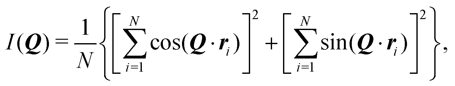
The kinetics of RM self-assembly were studied in a 50-ns simulation of 1000 AOT molecules in cyclohexane, with ω = 5, at P = 1 atm and T = 298.15 K. Snapshots from this simulation are shown in Fig. 4. At short times, there are many irregular clusters, while at longer times, the structure evolves into quite distinct RMs. By eye, there are about 45 to 50 distinct RMs, and given that there are 1000 AOT molecules, this translates to an aggregation number N_agg ≃ 20.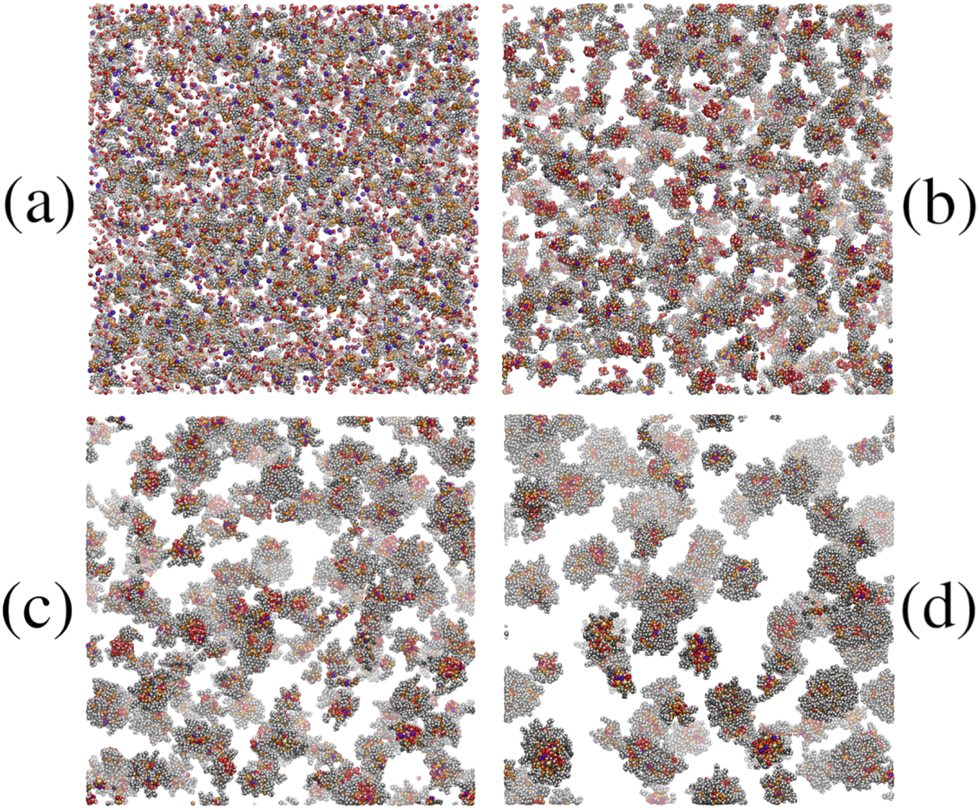

Fig. 4 Snapshots from the 1.7-million-atom simulation of AOT and water (ω = 5) in cyclohexane at P = 1 atm and T = 298.15 K: (a) 0 ns; (b) 2 ns; (c) 10 ns; (d) 50 ns. The solvent molecules are hidden for the sake of clarity, the AOT carbons are dark grey, the AOT oxygens are orange, the water oxygens are red, the water hydrogens are white, sulfur atoms are yellow, and sodium ions are violet.

The aggregation was tracked not by counting clusters or RMs, but rather by estimating the concentration of self-assembled objects in terms of the computed scattering. The problem with counting aggregates is that suitable criteria for clusters and RMs will be different, and there is the additional complication of whether water is present or not in aggregates at any given moment. Another measure could be the degree of association (the fraction of molecules associated with at least one other molecule), but this will be insensitive to the crossover from clusters to RMs. To get around this problem, the apparent scattering at a given time was computed and fitted. The equivalent of I(Q) in the simulation was calculated using the formula⁵⁰

where r_i is the position vector of particle i, and N is the total number of atoms in AOT and water. The wave vectors are commensurate with the periodic boundary conditions, and given by Q = 2π(n_x,n_y,n_z)/L, where n_α = 0, ±1, ±2,…. Since the system is isotropic, values of I with equal Q = |Q| were averaged. As defined, I(Q) → N as Q → 0, and I(Q) → 1 as Q → ∞. I(Q) was fitted using eqn (3) with assumed functions for P(Q) and S(Q). The structure factor was taken to be that for hard spheres at low concentration; in this case, the pair correlation function between spheres of diameter D is h(r) = −1 when r ≤ D, and h(r) = 0 otherwise.⁵⁰ The corresponding structure factor iswhere c is the concentration of RMs. The form factor can be taken from various structural models, but here the most relevant ones are a hard spherethe Gaussian model (eqn (5)), and a spherical particle with an exponential density profileSince I(Q) and S(Q) approach one at high Q, then so must P(Q). This was enforced by defining P(Q) = [P(0) − 1]f(Q) + 1, where f(Q) is the right-hand side of eqn (5), (8), or (9). This is just a correction for an object containing a fixed number of points, rather being a uniform object. Note that the hard-sphere radius, hard-sphere diameter, and radius of gyration are linked by . To reduce scatter in the data, the 50-ns simulation was divided up into 1-ns segments, and the scattering was computed and averaged over each segment.

Fig. 5 shows I(Q) computed from the final 1-ns segment, along with fits to eqn (3) using three different assumed form factors: the Gaussian function (eqn (5)); the exponential function (eqn (9)); and the hard-sphere function (eqn (8)). The corresponding values of R_g are given in the figure. From the single-RM simulations, the value of R_g is between 15 and 16 Å, between the Gaussian and exponential-fit values. In the case of the Gaussian fit, the corresponding factors of P(Q) and S(Q) are also shown, and the difference between P(Q) and I(Q) illustrates the importance of including S(Q). Given that the Gaussian fit provides an excellent description of the experimental and single-RM simulations, and that R_g is slightly too small because the simulation may not have fully reached equilibrium (50 ns was the maximum that could be achieved with the computational resources), this fit is used in what follows. Note that the results only differ by a few Å, and that the most important results from the other two types of fit will also be presented.

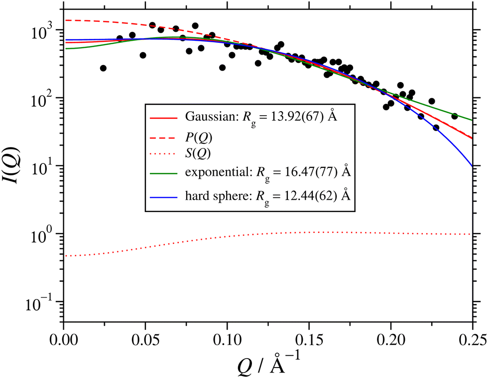Fig. 5 Simulated scattering intensity I(Q) from the final 1-ns segment of the 1.7-million-atom simulation of AOT and water (ω = 5) in cyclohexane at P = 1 atm and T = 298.15 K. The simulation results are shown as points, and fits with various assumed form factors are shown as solid lines. In the case of the Gaussian fit, the corresponding P(Q) and S(Q) are also shown as dashed lines and dotted lines, respectively.

Fig. 6(a) and (b) show the evolution of the apparent hard-sphere and gyration radii over the 50-ns simulation. In each case, there is an initial rise over the first 20 ns, and then it levels off. Fitting the results over the last 10 ns gives the values R_HS ≃ 18 Å and R_g ≃ 14 Å. As noted above, these values are slightly smaller than those obtained from experiment and single-RM simulations, but the differences are small. Fig. 6(c) shows the aggregate concentration c as a function of time. This decreases during self-assembly due to the merging of smaller clusters into RMs. This could be fitted with the simple exponential function

c(t) = [c(0) − c(∞)]e^−t/τ + c(∞), (10)

where c(0) is the initial concentration, c(∞) is the final concentration, and τ is a characteristic assembly time. The first few points suggest a more rapid, initial decrease than the asymptotic one, but fitting a two-exponential function worsens the fit, and gives a negative value of c(∞). In any case, the error bars in the first few points are large, and the fit was weighted accordingly, so they do not influence the result significantly. The single-exponential fit yields an assembly time τ ≃ 15 ns, and a final aggregate concentration c(∞) = 2.99 × 10²⁴ m⁻³. The aggregation number is plotted as a function of time in Fig. 6(d). The points are the overall AOT concentration, c_AOT = 5.76 × 10²⁵ m⁻³, divided by the `instantaneous' values of c, and are shown along with a plot of the function N_agg = c_AOT/c(t). Asymptotically, the aggregation number is predicted to approach c_AOT/c(∞) ≃ 19.3, close to the value estimated by eye.

Fig. 6 Aggregation parameters as functions of time from the 1.7-million-atom simulation of AOT and water (ω = 5) in cyclohexane at P = 1 atm and T = 298.15 K: (a) the aggregate hard-sphere radius; (b) the aggregate radius of gyration; (c) the aggregate concentration; (d) the aggregation number. The points are from fitting the Gaussian scattering model to the simulation results in 1-ns segments, the blue solid lines are fits, and the dashed red lines are asymptotic values.

Exactly the same analysis was carried out using the other two form factors – exponential and hard-sphere – and all of the results are compiled in Table 3. The results show that the apparent RM radius and aggregation number increase by using, in order, hard-sphere, Gaussian, and exponential form factors in fitting I(Q), but that the Gaussian and exponential values bracket those from experiments and single-RM simulations. It was already noted that the simulation may not have fully reached equilibrium, and there may be much slower assembly kinetics – akin to Ostwald ripening – that are beyond the reach of simulations of this size. For example, the growth of RMs may involve a combination of merging, AOT and water dissolution, and subsequent reassembly. Nonetheless, the assembly time within the 50-ns window is consistently in the range 15–16 ns, showing that the choice of form factor is not important in assessing the short-time kinetics.

Table 3 Parameters describing the self-assembly kinetics from the 1.7-million-atom simulation of AOT and water (ω = 5) in cyclohexane at P = 1 atm and T = 298.15 K. R_HS and R_g are averages from the last 10 ns of the simulation, c(∞) and τ are fit parameters from eqn (10), and N_agg = c_AOT/c(∞), where c_AOT is the total AOT-molecule concentration

Model	R HS/Å	R g/Å	c(∞)/10^24 m^−3	τ/ns	N agg
Gaussian	18.11 ± 0.13	14.02 ± 0.10	2.99 ± 0.26	15.0 ± 2.0	19.3 ± 1.7
Exponential	21.14 ± 0.20	16.37 ± 0.16	2.06 ± 0.21	15.6 ± 2.1	27.9 ± 2.8
Hard sphere	16.30 ± 0.09	12.67 ± 0.07	3.58 ± 0.36	15.7 ± 2.3	16.1 ± 1.6

---

3.4 Effects of solvent and water content on reverse-micelle structure

The internal structures of the RMs were characterized with radial mass-density profiles ρ(r) for the sodium cations, and groups of atoms on the AOT anions, solvent molecules, and any added water. This was computed by identifying atoms at radial distances between r and r + δr from the centre of mass of the RM, with δr = 0.5 Å, allocating each atom to one species, and computing the local mass density for each species by dividing the mass by the volume 4π[(r + δr)³ − r³]/3 ≈ 4πr²δr. Results from the N_AOT = 40 simulations in cyclohexane and dodecane with ω = 5 are shown in Fig. 7(a) and (b), respectively. Note that the radius of gyration of the RM (from Table 1) corresponds roughly to where the AOT-anion and solvent density profiles overlap. In both solvents, the core of the RM contains the water and sodium cations, the AOT anions are localized in a shell between the core and surrounding solvent, and the solvent partially penetrates the RM. The solvent mass-density profiles reach the expected bulk values at large value of r: the experimental mass densities of cyclohexane and dodecane are 774 kg m⁻³ and ρ = 746 kg m⁻³, respectively;⁵¹ fitting the constant portions of the simulated mass-density profiles gives 759 ± 6 kg m⁻³ and ρ = 744 ± 3 kg m⁻³, respectively, reflecting the typical accuracy of the OPLS-AA force field. Once stabilized, the internal structures of the micelles appear similar regardless of solvent. However, the self-assembly dynamics vary noticeably from one solvent to another. While in cyclohexane the equilibration process takes only 10–15 ns, the dodecane systems took significantly longer to stabilize, approaching 50 ns. There was also the possibility of further increases in the aggregation number on longer time scales, beyond the scope of the current study. The difference in behaviour may be due to the dodecane being linear and more chemically similar to the aliphatic chains of the AOT tails, unlike the cyclic structure of cyclohexane.

Fig. 7 Radial mass-density profiles showing comparisons between the internal structures of RMs formed in N_AOT = 40 simulations in (a) cyclohexane and (b) dodecane with ω = 5. The dotted black lines are the fitted bulk-phase densities of the solvents.

Next is an examination of the effects of the hydration ratio on the RM structure. Previous simulation studies on AOT¹⁷ and other surfactants^49,52,53 in non-polar solvents show that the presence or absence of water can significantly affect the RM size, structure, and behaviour at interfaces. Fig. 8 shows a comparison of mass density profiles for AOT in cyclohexane with ω = 1 and ω = 60. With ω = 1 (N_agg = 9), the water forms a dense core and a less-dense shell, and the sodium cations remain close to the water. In contrast, with ω = 60 (N_agg = 30) there is sufficient water that its density is nearly constant within the core, at ρ ≃ 1050 kg m⁻³. The sodium cations are distributed within the water core fairly uniformly, rather than being strongly associated with the AOT anions. There is a slight increase in the density profile at the interface between the water and the AOT-anion shell, suggesting that there is still some association between the cations and the surfactant head groups. Another interesting difference is that the AOT shell appears more distinct at ω = 1 than with ω = 60. There is an increase of the water-solvent overlap with the increased hydration ratio, and the AOT shell gets less dense and more spread out. While the number of AOT molecules is also larger with a larger hydration ratio, the packing density of those molecules within the shell need not stay the same, and indeed the actual mass density (peak height) does decrease with increasing ω. Another factor is that with a lower value of ω, a greater proportion of water molecules is strongly associated with the AOT head groups, and this also leads to a stronger structural distinction between core, shell, and surrounding solvent.

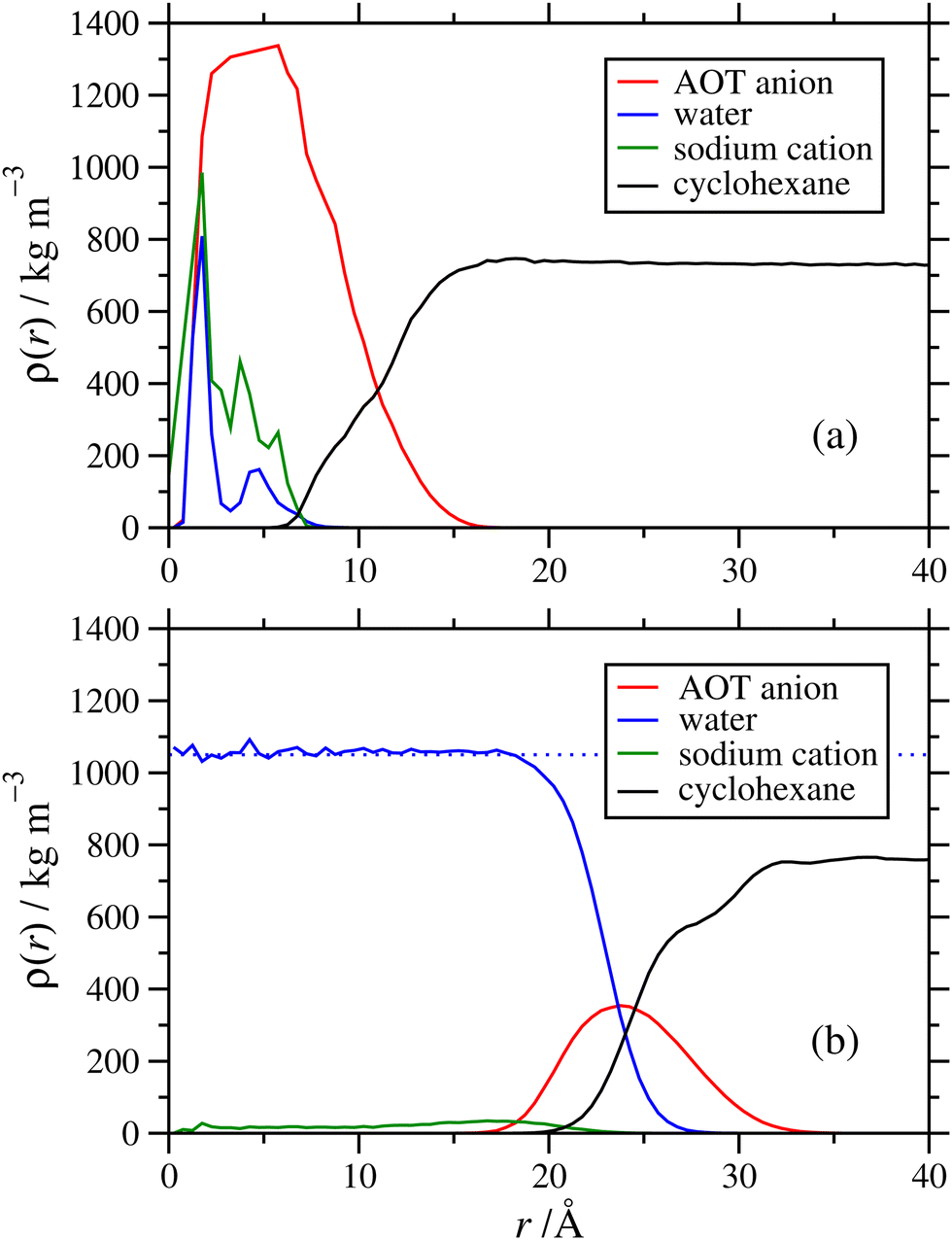Fig. 8 Radial density profiles showing comparisons between the internal structures of RMs formed in N_AOT = 30 simulations in cyclohexane with (a) ω = 1 and (b) ω = 60. In (b), the dotted blue line is the fitted bulk-phase density of water.

3.5 Water dynamics

An interesting question is the nature of the water inside the RMs, which have long been studied as ‘microreactors’ for chemical reactions,¹¹ sequestration and delivery media, etc. With low values of the hydration ratio, the water should be strongly coordinated to the polar head groups and ions of the surfactant, and as the hydration ratio is increased, the proportion of bulk-like water should grow. This has been studied before using combinations of quasi-elastic neutron scattering, NMR spectroscopy, and MD simulations.^{9,12,13,17,22,23,54,55} Here, the reorientational dynamics of the water molecules are analyzed briefly. Much more detailed studies have been carried out on larger preformed RMs of AOT with water in isooctane.¹⁷ When a water molecule is coordinated to surfactant, its rotation should be slaved to that of the surfactant and the RM as a whole, and so the effective Debye relaxation time should be large as compared to bulk water. The reorientational dynamics were studied using the single-molecule dipole autocorrelation functionwhere the angled brackets denote an average over water molecules, and as defined, C(0) = 1. Simulations of RMs in cyclohexane with hydration ratios ω = 1–60 were carried out, as listed in Table 1. The results are shown in Fig. 9(a) on log-linear scales. The straight lines at long times show that C(t) decays exponentially, and that the slope increases (relaxation time decreases) with increasing ω. Fig. 9(a) also includes results from a simulation of pure water using the TIP3P (Ewald) force field.⁴²

Fig. 9 (a) Reorientational correlation functions C(t) and (b) asymptotic relaxation times, for water encapsulated in the cores of RMs in N_AOT = 30 simulations in cyclohexane. In (a), ln C(t) is plotted against t to highlight the long-time, exponential decay of the correlation function. The lines are fits using eqn (12). In (b), τ₂ (the longer of two relaxation times) is plotted against 1/ω. The line is a linear fit, with intercept τ₂ ≃ 4.2 ps.

It was found that the results could be fitted quite accurately using the two-timescale function

C(t) = (1 − f)exp(−t/τ₁) + fexp (−t/τ₂), (12)

where τ₁ and τ₂ are characteristic relaxation times, and (1 − f) and f reflect the respective contributions. The fit parameters are shown in Table 4. First, the contribution from the shorter-timescale relaxation is much the smaller of the two. Second, both timescales decrease with increasing ω; the values with ω = 1 will not be very reliable, because of the number of water molecules, and the strong coordination with the surfactant ions. Finally, the longest timescale decreases from 10s or 100s of picoseconds, down to a few picoseconds as ω is increased. The results for τ₂ are plotted in Fig. 9(b) as a function of ω⁻¹, which gives a roughly straight line; a linear fit gives an intercept of τ₂ = (4.2 ± 0.2) ps. It is known that in bulk water, the Debye relaxation time is τ_D = 9.3 ps,⁵⁶ but this is the relaxation time for the dielectric polarization of the liquid, not a single molecule, and so this should be longer than the single-molecule relaxation time because of collective effects. Note that the dielectric spectrum of liquid water contains many high-frequency features associated with various kinds of motions, including a ‘fast Debye process’ with τ ≃ 1 ps, and even faster processes associated with bond-bending, bond-stretching, and librational motions.⁵⁶

Table 4 Fit parameters from eqn (12) for the single-dipole reorientational dynamics of water in AOT RMs in cyclohexane with hydration ratio ω. The results at ω = ∞ are for pure bulk water

ω	f	τ 1/ps	τ 2/ps
1	0.822 ± 0.002	0.20 ± 0.01	129 ± 6
5	0.781 ± 0.004	0.48 ± 0.03	23.0 ± 0.4
10	0.759 ± 0.005	0.64 ± 0.04	20.9 ± 0.5
15	0.815 ± 0.003	0.36 ± 0.02	14.2 ± 0.2
60	0.758 ± 0.005	0.52 ± 0.03	8.6 ± 0.1
∞	0.839 ± 0.002	0.23 ± 0.01	4.13 ± 0.01

---

4 Conclusions

In this work, reverse-micelle formation by aerosol-OT and water in non-polar solvents has been studied using a combination of experimental and molecular-simulation methods. New small-angle neutron scattering data indicate the formation of reverse micelles in cyclohexane and in dodecane. The apparent dimensions of the reverse micelles were extracted by fitting various assumed form factors. Molecular simulations were used to examine reverse-micelle formation in the same solvents, and with varying water concentrations. An essential feature of the simulations is that the reverse micelles are not preassembled. Rather, the aim was to observe spontaneous reverse-micelle formation on the simulation time scale. To this end, conventional force fields had to be adapted, in particular to account for the partial charges on the surfactant head group. This was achieved successfully using density functional theory calculations, and with the resulting force field, the final dimensions of the reverse micelles were in excellent agreement with experimental values. Most of the simulations were with single (meaning isolated) reverse micelles, but a 1.7-million-atom simulation was carried out that, after 50 ns, contained around 50 reverse micelles. An analysis of the kinetics indicates that the characteristic assembly time (associated with the decrease in the number of reverse micelles) was around 15 ns. Additional investigations were focused on the organization of the water, cation, surfactant anion, and solvent within the reverse micelles, and the reorientational dynamics of the water within the reverse-micelle cores.

This work can be developed in several other directions. Firstly, the study was focused on spherical reverse micelles of aerosol-OT in cyclohexane and dodecane, and the structures were very similar in both cases. In ongoing work with dodecane and at high water contents, beyond those presented here, neutron-scattering measurements indicate the formation of rod-like structures. The results will be reported as part of an experimental and simulation study of aerosol-OT adsorption at the solid–oil interface. Secondly, aerosol-OT exhibits a well-defined critical micelle concentration,⁸ and this could be studied with simulations through either direct computations of the cluster-size distributions,⁵⁷ fitting simulation data to thermodynamic models,⁵⁸ or computing the interfacial tension as a function of surfactant concentration.⁵⁹ Finally, to go beyond current comprehensive simulations of water inside reverse micelles,¹⁷ and incorporate proton equilibria and dynamics, would require quantum-mechanical techniques.

In summary, molecular simulations validated against new experimental measurements have shown that it is possible to simulate the spontaneous self-assembly, structures, and dynamical properties of reverse micelles formed by a well-known anionic surfactant, and water, in non-polar solvents.

Author contributions

Conceptualization: AM, GM, PJD, JE, PJC. Data curation: AM, GM, PJC. Formal analysis: AM, GM, PJC. Funding acquisition: PJD, JE, PJC. Investigation: AM, GM. Methodology: AM, GM, PJD, JE, PJC. Project administration: PJD, JE, PJC. Resources: PJD, JE, PJC. Software: AM, PJC. Supervision: PJD, JE, PJC. Validation: AM, GM, PJC. Visualization: AM, PJC. Writing – original draft: AM, PJC. Writing – review & editing: AM, GM, PJD, JE, PJC.

Data availability

Data for this article, including raw MD and SANS results, are available from Edinburgh DataShare at https://doi.org/10.7488/ds/7824.

Conflicts of interest

There are no conflicts to declare.

Acknowledgements

This research was supported by Infineum UK Ltd through studentships for AM (jointly with the Engineering and Physical Sciences Research Council Projects EP/N509644/1 and EP/R513209/1) and GM. AM and PJC thank Dr Julien Sindt and Dr Rui Apóstolo (EPCC, Edinburgh) for help with benchmarking, testing, monitoring, and post-processing the large-scale simulation on ARCHER2. GM and JE acknowledge the support of instrument scientists Dr Sarah E. Rogers (ISIS) and Dr Sylvain Prévost (ILL), and ILL, ISIS, and the Science and Technology Facilities Council (UK) for the allocation of beam time, and funding for travel and consumables.

Notes and references

1. C. R. Caryl and A. O. Jaeger, Detergent Composition, U.S. Pat., 2181087, 1939.
2. A. J. Singer, E. Sauris and A. W. Viccellio, Ann. Emerg. Med., 2000, 36, 228–232.
3. D. K. Kaczmarek, T. Rzemieniecki, K. Marcinkowska and J. Pernak, J. Ind. Eng. Chem., 2019, 78, 440–447.
4. J. Eastoe, G. Fragneto, B. H. Robinson, T. F. Towey, R. K. Heenan and F. J. Leng, J. Chem. Soc., Faraday Trans., 1992, 88, 461–471.
5. T. K. De and A. Maitra, Adv. Colloid Interface Sci., 1995, 59, 95–193.
6. J. Eastoe, M. J. Hollamby and L. Hudson, Adv. Colloid Interface Sci., 2006, 128–130, 5–15.
7. M. J. Hollamby, R. Tabor, K. J. Mutch, K. Trickett, J. Eastoe, R. K. Heenan and I. Grillo, Langmuir, 2008, 24, 12235–12240.
8. G. N. Smith, P. Brown, S. E. Rogers and J. Eastoe, Langmuir, 2013, 29, 3252–3258.
9. S. J. Law and M. M. Britton, Langmuir, 2012, 28, 11699–11706.
10. C. Petit, P. Lixon and M.-P. Pileni, J. Phys. Chem., 1993, 97, 12974–12983.
11. M.-P. Pileni, J. Phys. Chem., 1993, 97, 6961–6973.
12. G. Kassab, D. Petit, J.-P. Korb, T. Tajouri and P. Levitz, C. R. Chim, 2010, 13, 394–398.
13. T. L. Spehr, B. Frick, M. Zamponi and B. Stühn, Soft Matter, 2011, 7, 5745–5755.
14. S. Nave, J. Eastoe and J. Penfold, Langmuir, 2000, 16, 8733–8740.
15. S. Abel, F. Sterpone, S. Bandyopadhyay and M. Marchi, J. Phys. Chem. B, 2004, 108, 19458–19466.
16. S. Abel, M. Waks, W. Urbach and M. Marchi, J. Am. Chem. Soc., 2006, 128, 382–383.
17. M. Crowder, F. Tahiry, I. Lizarraga, S. Rodriguez, N. Peña and A. K. Sharma, J. Mol. Liq., 2023, 375, 121340.
18. J. Faeder and B. M. Ladanyi, J. Phys. Chem. B, 2000, 104, 1033–1046.
19. J. Faeder and B. M. Ladanyi, J. Phys. Chem. B, 2001, 105, 11148–11158.
20. J. Faeder, M. V. Albert and B. M. Ladanyi, Langmuir, 2003, 19, 2514–2520.
21. J. Faeder and B. M. Ladanyi, J. Phys. Chem. B, 2005, 109, 6732–6740.
22. M. R. Harpham, B. M. Ladanyi and N. E. Levinger, J. Phys. Chem. B, 2005, 109, 16891–16900.
23. D. E. Rosenfeld and C. A. Schmuttenmaer, J. Phys. Chem. B, 2006, 110, 14304–14312.
24. A. V. Nevidimov and V. F. Razumov, Mol. Phys., 2009, 107, 2169–2180.
25. V. R. Vasquez, B. C. Williams and O. A. Graeve, J. Phys. Chem. B, 2011, 115, 2979–2987.
26. R. Urano, G. A. Pantelopulos and J. E. Straub, J. Phys. Chem. B, 2019, 123, 2546–2557.
27. S. Plimpton, J. Comput. Phys., 1995, 117, 1–19.
28. A. P. Thompson, H. M. Aktulga, R. Berger, D. S. Bolintineanu, W. M. Brown, P. S. Crozier, P. J. in't Veld, A. Kohlmeyer, S. G. Moore, T. D. Nguyen, R. Shan, M. J. Stevens, J. Tranchida, C. Trott and S. J. Plimpton, Comput. Phys. Commun., 2022, 271, 108171.
29. LAMMPS Molecular Dynamics Simulator, 2024, https://www.lammps.org.
30. M. P. Allen and D. J. Tildesley, Computer Simulation of Liquids, Oxford University Press, Oxford, 2nd edn, 2016.
31. W. L. Jorgensen, J. D. Madura and C. J. Swenson, J. Am. Chem. Soc., 1984, 106, 6638–6646.
32. W. L. Jorgensen and J. Tirado-Rives, J. Am. Chem. Soc., 1988, 110, 1657–1666.
33. W. L. Jorgensen, D. S. Maxwell and J. Tirado-Rives, J. Am. Chem. Soc., 1996, 118, 11225–11236.
34. W. Damm, A. Frontera, J. Tirado-Rives and W. L. Jorgensen, J. Comput. Chem., 1997, 18, 1955–1970.
35. S. W. I. Siu, K. Pluhackova and R. A. Böckmann, J. Chem. Theory Comput., 2012, 8, 1459–1470.
36. W. L. Jorgensen and J. Tirado-Rives, Proc. Natl. Acad. Sci. U. S. A., 2005, 102, 6665–6670.
37. L. S. Dodda, J. Z. Vilseck, J. Tirado-Rives and W. L. Jorgensen, J. Phys. Chem. B, 2017, 121, 3864–3870.
38. L. S. Dodda, I. Cabeza de Vaca, J. Tirado-Rives and W. L. Jorgensen, Nucleic Acids Res., 2017, 45, W331–W336.
39. LigParGen, 2024, https://traken.chem.yale.edu/ligpargen/.
40. J. A. Rackers, Z. Wang, C. Lu, M. L. Laury, L. Lagardère, M. J. Schnieders, J.-P. Piquemal, P. Ren and J. W. Ponder, J. Chem. Theory Comput., 2018, 14, 5273–5289.
41. Tinker - Software Tools for Molecular Design, 2024, https://dasher.wustl.edu/tinker/.
42. D. J. Price and C. L. Brooks, III, J. Chem. Phys., 2004, 121, 10096–10103.
43. R. J. Good and C. J. Hope, J. Chem. Phys., 1970, 53, 540–543.
44. S. Abdel-Azeim, J. Chem. Theory Comput., 2020, 16, 1136–1145.
45. M. J. Frisch, G. W. Trucks, H. B. Schlegel, G. E. Scuseria, M. A. Robb, J. R. Cheeseman, G. Scalmani, V. Barone, G. A. Petersson, H. Nakatsuji, X. Li, M. Caricato, A. V. Marenich, J. Bloino, B. G. Janesko, R. Gomperts, B. Mennucci, H. P. Hratchian, J. V. Ortiz, A. F. Izmaylov, J. L. Sonnenberg, D. Williams-Young, F. Ding, F. Lipparini, F. Egidi, J. Goings, B. Peng, A. Petrone, T. Henderson, D. Ranasinghe, V. G. Zakrzewski, J. Gao, N. Rega, G. Zheng, W. Liang, M. Hada, M. Ehara, K. Toyota, R. Fukuda, J. Hasegawa, M. Ishida, T. Nakajima, Y. Honda, O. Kitao, H. Nakai, T. Vreven, K. Throssell, J. A. Montgomery, Jr., J. E. Peralta, F. Ogliaro, M. J. Bearpark, J. J. Heyd, E. N. Brothers, K. N. Kudin, V. N. Staroverov, T. A. Keith, R. Kobayashi, J. Normand, K. Raghavachari, A. P. Rendell, J. C. Burant, S. S. Iyengar, J. Tomasi, M. Cossi, J. M. Millam, M. Klene, C. Adamo, R. Cammi, J. W. Ochterski, R. L. Martin, K. Morokuma, O. Farkas, J. B. Foresman and D. J. Fox, Gaussian 16 Revision C.01, Gaussian Inc., Wallingford CT, 2016.
46. L. Martínez, R. Andrade, E. G. Birgin and J. M. Martínez, J. Comp. Chem., 2009, 30, 2157–2164.
47. PACKMOL, 2024, https://m3g.github.io/packmol/, 2024.
48. M. Tolan, X-Ray Scattering from Soft-Matter Thin Films, Springer Berlin Heidelberg, Berlin, Heidelberg, 1st edn, 1999, vol. 148, p. 198.
49. J. L. Bradley-Shaw, P. J. Camp, P. J. Dowding and K. Lewtas, J. Phys. Chem. B, 2015, 119, 4321–4331.
50. J.-P. Hansen and I. R. McDonald, Theory of Simple Liquids, Academic Press, London, 3rd edn, 2006.
51. E. W. Lemmon, I. H. Bell, M. L. Huber and M. O. McLinden, NIST Chemistry WebBook, NIST Standard Reference Database Number 69, National Institute of Standards and Technology, Gaithersburg MD, 20899, 2023.
52. J. L. Bradley-Shaw, P. J. Camp, P. J. Dowding and K. Lewtas, Langmuir, 2016, 32, 7707–7718.
53. J. L. Bradley-Shaw, P. J. Camp, P. J. Dowding and K. Lewtas, Phys. Chem. Chem. Phys., 2018, 20, 17648–17657.
54. M. R. Harpham, B. M. Ladanyi, N. E. Levinger and K. W. Herwig, J. Chem. Phys., 2005, 121, 7855–7868.
55. B. Baruah, J. M. Roden, M. Sedgwick, N. M. Correa, D. C. Crans and N. E. Levinger, J. Am. Chem. Soc., 2006, 128, 12758–12765.
56. I. Popov, P. Ben Ishai, A. Khamzin and Y. Feldman, Phys. Chem. Chem. Phys., 2016, 18, 13941–13953.
57. A. P. Santos and A. Z. Panagiotopoulos, J. Chem. Phys., 2016, 144, 044709.
58. A. Del Regno, P. B. Warren, D. J. Bray and R. L. Anderson, J. Phys. Chem. B, 2021, 125, 5983–5990.
59. H. Cárdenas, M. Ariif, H. Kamrul-Bahrin, D. Seddon, J. Othman, J. T. Cabral, A. Mejía, S. Shahruddin, O. K. Matar and E. A. Müller, J. Colloid Interface Sci., 2024, 674, 1071–1082.

---

Footnotes

† Electronic supplementary information (ESI) available: Force-field parameters for the Aerosol-OT molecule. See DOI: https://doi.org/10.1039/d4cp03389b

‡ Present address: Department of Pure and Applied Chemistry, University of Strathclyde, Glasgow G1 1XL, Scotland, UK.

---