
 Open Access Article
 This Open Access Article is licensed under a
 Creative Commons Attribution 3.0 Unported Licence
Modeling interfacial electric fields and the ethanol oxidation reaction at electrode surfaces†
Yuhan
Mei
a,
Fanglin
Che
b and
N. Aaron
Deskins
 *a
*a
aDepartment of Chemical Engineering, Worcester Polytechnic Institute, Worcester, Massachusetts 01609, USA. E-mail: nadeskins@wpi.edu
bDepartment of Chemical Engineering, University of Massachusetts Lowell, Lowell, Massachusetts 01854, USA
First published on 21st October 2024
Abstract
The electrochemical environment present at surfaces can have a large effect on intended applications. Such environments may occur, for instance, at battery or electrocatalyst surfaces. Solvent, co-adsorbates, and electrical field effects may strongly influence surface chemistry. Understanding these phenomena is an on-going area of research, especially in the realm of electrocatalysis. Herein, we modeled key steps in the ethanol oxidation reaction (EOR) over a common EOR catalyst, Rh(111), using density functional theory. We assessed how the presence of electrical fields may influence important C–C and C–H bond scission and C–O bond formation reactions with and without co-adsorbed water. We found that electric fields combined with the presence of water can significantly affect surface chemistry, including adsorption and reaction energies. Our results show that C–C scission (necessary for the complete oxidation of ethanol) is most likely through CHxCO adsorbates. With no electric field or solvent present C–C scission of CHCO has the lowest reaction energy and dominates the oxidation of ethanol. But when applying strong negative fields (with or without solvent), the C–C scission of CH2CO and CHCO becomes competitive. The current work provides insights into how electric fields and water solvent affect EOR, especially when simulated using density functional theory.
1 Introduction
The growing demand for energy and the consumption of non-renewable fossil fuels have a negative impact on the environment. Fuel cells are widely regarded as a cleaner alternative energy technology. In particular, ethanol has attracted considerable interest as a fuel source due to its abundant availability from biomass feedstocks.1,2 Compared to other fuels, ethanol is also less toxic, has a higher boiling point, and possesses a high energy density comparable to that of gasoline.3–8 The complete ethanol oxidation reaction (EOR), which is ideal for maximizing electron production, involves efficient C–H and C–C bond cleavage leading to CO2 as the final product.9–11 On the other hand, incomplete EOR involves hydrogen removal and potential C–O bond formation (while avoiding C–C scission), resulting in by-products such as acetaldehyde and acetic acid.12,13 Slow C–C bond scission (essential for complete EOR) at the anode catalyst (typically transition metals) limits the commercial viability of direct ethanol fuel cells (DEFCs). Since EOR occurs in an electrochemical environment, a thorough understanding of the relationship between surface chemistry and reaction environment is critical to the scientific advancement of EOR catalysts.Density functional theory (DFT) is a powerful tool for simulating electrochemical interfaces, which is the primary method used in the current study. There are various approaches to modeling electrochemical interfaces and describing the various components present at the interface (e.g., solvent molecules, electric fields, electron potential, etc.).14–16 A common technique to account for the electrode potential is to simulate electrocatalytic hydrogen/electron transfer at metal surfaces by adding energy adjustments based on the electron potential at the electrode surface, also known as the computational hydrogen electrode (CHE) approach.17 However, the widely used CHE method overlooks the effects of electric fields present near the electrode surface. Such fields can significantly alter the surface chemistry and affect adsorbate interactions. Furthermore, C–C bond cleavage does not involve hydrogen/electron transfer, and thus the electric field and solvent molecules near the electrode surface are expected to influence C–C bond cleavage more than the potential of the electrons themselves. Other methods exist for modeling electrochemical systems, such as the computational standard hydrogen electrode (SHE)18,19 method, which determines redox potentials using ab initio molecular dynamics (AIMD). Such calculations can be time-consuming, and controlling local electric fields with this method can be difficult. A related method is the constant-potential hybrid-solvation dynamic model20,21 which also uses AIMD and requires varying the number of electrons added to or removed from the system to maintain a constant applied potential. One prominent method to simulate the electric fields present at electrochemical systems is to introduce a dipole sheet into the vacuum, which creates an electric field in the simulation cell.22
Various DFT papers have examined the effect of an electrical field on surface chemistry.23–28 Electric fields can lead to remarkable behavior and variations in catalyst efficiency.23,24,29–34 It should be noted that it is possible to relate the electric field strength near the electrode surface to the electrode potential, as the electrode potential can be approximated as the double-layer thickness multiplied by the field strength, illustrated by Rossmeisl et al.23 A similar approach was used by Karlberg et al.31 Haruyama et al.35 also developed methods to relate electric fields to the electrode potentials. In other DFT studies on the oxygen reduction reaction,24,31,36 electric fields were incorporated to improve the simulations. Electric fields were also included in studies of methane conversion.25,37,38 Estejab et al.39 modeled methanol oxidation in the presence of an electric field. Regarding the study of electric fields in ethanol oxidation reactions, Jiang et al.26 have used molecular dynamics simulations to investigate the effect of external electric fields of different strengths on EOR (albeit in the gas phase without the presence of a catalyst). Their study shows that the application of an electric field not only changes the reaction rate in a nonlinear manner, but also modifies the reaction pathways for ethanol oxidation.
Previous studies have used molecular modeling approaches to better understand the role of electric fields in C–C and C–H bond cleavage (important for many reactions involving organic species). Investigations by Che et al. examined the effect of electric fields on C–H bond cleavage of CHx (x = 1–3) species over Ni,40,41 suggesting that negative external electric fields lower energy barriers while positive fields raise them. In recent work, Zhou et al.42 reported that for gas-phase pyrolysis of n-alkanes, electric fields can promote the breaking of C–C and C–H bonds. As for the C–C and C–H bond breakings in EOR, complementary studies using reactive force field (ReaxFF) molecular dynamics simulations have also been performed,26,27 analyzing the effects of external electric fields on the ethanol oxidation reaction mechanisms in the absence of a catalyst and in an O2 gas environment. These modeling efforts suggest that electric fields can shift reaction mechanisms and possibly open alternative reaction pathways for oxidation of alcohols like ethanol. However, the precise influence of an external electric field on surface-mediated reactions relevant to complete ethanol oxidation, which involves the breaking of both C–C and C–H bonds, remains an open question in the context of DFT simulations.
In addition to electric fields present at electrocatalyst surfaces, solvent molecules can also alter catalyst reactivity. In particular, the solvation environment can be instrumental in facilitating various surface reactions, including both oxidation and electrocatalytic processes. Several studies focused on solvation effects and bond dissociation reactions on metal surfaces. Investigations by Schweitzer et al.43 and Gu et al.44 have shown that accounting for water solvation can significantly alter the cleavage of C–C and C–H bonds in ethanol on a Pt(111) surface. Estejab et al. modeled methanol oxidation with explicit water molecules under an electric field. They indicated a dependency of both the solvation energy and the entropy on the strength and direction of an electric field, with the entropy of solvation being significantly impacted due to the orientation of water molecules.39 Complementary findings by Mei et al.45 highlighted the substantial role of a water solvent in modifying the dissociation of the C–C/C–H bonds on Rh(111). In a previous study, Guo et al.46 used DFT coupled with an implicit continuum solvation model to investigate the potential-dependent mechanism of EOR on Pd. They proposed a mechanism where C–C bond scission changed only slightly under different potentials. In light of these previous findings, the current study aims to unravel the interactive effects of both the explicit presence of water and electric fields on EOR.
We investigated the influence of electric fields on EOR using DFT to model the Rh(111) surface, which has been previously recognized as an effective catalyst for EOR.7,10,47–53 We calculated the reaction energies for key EOR steps: C–C and C–H bond cleavage and C–O bond formation. Although there are numerous computational strategies for simulating electric fields,54–61 our approach was to apply an external electric field following the methodology established by Neugebauer and Scheffler,22 where a dipole sheet is inserted into the vacuum layer. Given that our focus is primarily on examining the effects of local electric fields, the dipole sheet method is both sufficient and computationally less expensive than other methods. Thus, we can simulate the effect of an electric field on adsorbate-covered surfaces. In addition, our study incorporated a co-adsorbed water molecule from the solvent environment to determine its effect on the EOR. The inclusion of explicit water molecules is a more representative model of solvation than implicit solvent models, especially in the context of relevant EOR processes.43,45,52,62,63 Previous work39,55,58 has demonstrated how electric fields can be used in conjunction with explicit water molecules to understand electrochemical interfaces. Our work extends this to better understand the role of the electrochemical environment on EOR.
2 Methodology
2.1 Computational details
Our DFT calculations used the Vienna ab initio Simulation Package (VASP).64–67 Core electrons were described using the projector augmented wave (PAW) method.68,69 The number of valence electrons simulated for each atom was 9 for Rh, 4 for C, 1 for H, and 6 for O. We performed tests on the number of valence electrons for Rh (9 or 15) in our previous work and the results indicated that 9 electrons was suitable for our modeling of Rh.45 The Perdew–Burke–Ernzerhof (PBE) exchange–correlation functional70 was used throughout the study. The plane wave basis was expanded to an energy cutoff of 400 eV. First order Methfessel–Paxton smearing71 with a smearing width of 0.1 eV was also used. The convergence criteria for the self-consistent field (SCF) energy calculations and atomic forces were set to 10−5 eV and 0.03 eV Å−1, respectively. All calculations in this study were spin-polarized. Bader charges were calculated with the code of Henkelman et al.72–74The Rh(111) surface was represented by a (3 × 3) four-layer slab (as shown in Fig. 1), with cell lengths of 8.15 Å and a 10 Å vacuum separation set in the z direction perpendicular to the surface. The bottom two layers of the slab were fixed. The lattice constant of bulk Rh was calculated to be 3.84 Å, which is in agreement with previous work.9,10,51,75 For the slab calculations, a Gamma-centered k-point grid of 4 × 4 × 1 was chosen to sample reciprocal space. Gas phase molecules were modeled in a 20 Å × 20 Å × 20 Å box cell, and the gas phase calculations used a Monkhorst Pack k-point grid of 1 × 1 × 1.
 | ||
| Fig. 1 The slab model used in this work to represent the Rh(111) surface: (a) top view and (b) side view. The slab was a (3 × 3) slab with four layers, the bottom two layers being frozen. | ||
We modeled the adsorption of CH3CH2OH, CH3CH2O, CH2CH2O, CH2OH, CH2O, CH3CO, CH2CO, CHCO, CH3, CH2, CH, CO and H, as these species have been identified as key intermediates for the C–C and C–H bond breaking during ethanol oxidation/decomposition process.10,76,77 See also Fig. 2 for an illustration of various reactions and these species involved in EOR. In addition, we also modeled the adsorption of CH3COOH, CH3CO, and OH which are relevant for C–O bond formation. C–O bond formation can take place during incomplete EOR, and thus prevents complete EOR.12,13 Different initial geometries were considered in order to find stable configurations. Adsorbates were initially placed above the surface with atoms of the adsorbates at different fcc, hcp, top and bridge sites on the Rh(111) surface. The adsorption of larger molecules (e.g. CH3CH2OH, CH3CH2O, CH2CH2O, CH3CO, CH2CO, CHCO) can involve multiple interactions with the surface (e.g., *CH3CH2OH can have both of the C atoms interacting with Rh atoms). After geometry optimization, we took the structure with the lowest energy as the most stable configuration. For calculations in vacuum, geometries were first optimized without an external electric field, and then the most stable geometries were modeled in the presence of an external electric field in a range of −1.0 to 1.0 V Å−1, as discussed in the next section.
 | ||
| Fig. 2 Schematic representation of possible pathways for complete ethanol oxidation/decomposition on Rh(111).2,10,76,78,79 Key reactions involve C–C and C–H scission. Not shown are pathways for incomplete oxidation, leading to acetaldehyde, acetic acid, and possible other products. Further discussion of reactions modeled in this work is found in the Methodology section. | ||
2.2 External electric field
An external electric field perpendicular to the metal slab was applied using the method of Neugebauer and Scheffler.22 This method is implemented in VASP, and has been used in previous studies.30,80–82 Fig. S1 (ESI†) illustrates this method. As discussed in previous studies,30,82,83 the Neugebauer and Scheffler method introduces an artificial dipole sheet in the middle of the vacuum layer. We chose this method for its ability to assess the effects of local fields on surface chemistry, while remaining computationally efficient. The maximum electric field that can be introduced is limited by the height of the supercell due to “field emission” effects. An important requirement is to prevent the overlap between the electron density and the dipole sheet. Therefore, using the dipole sheet method requires a wide enough vacuum region. However, the vacuum must also not be too wide since a strong electric field will draw electrons out of the slab into the vacuum space and electrons may be found near the dipole sheet.30,83 Thus, in this work, applied electric fields had strengths up to ±1 V Å−1.Adsorption energies (ΔEads(F)) were calculated using this equation:30
| ΔE(F)ads = E(F)ads/slab − E(F)slab − E(F)ads(gas). | (1) |
To determine the impact of the electric field on surface reactions, we modeled several C–C and C–H bond breaking and C–O bond formation reactions over the Rh surface. We modeled C–C bond breaking involving CH3CH2OH, CH3CH2O, CH2CH2O, CH3CO, CH2CO, and CHCO. We also modeled C–H bond cleavage involving CH3CO and CH2CO. These reactions have been reported to be key reaction pathways in ethanol oxidation/decomposition.76,77,84,85 To calculate the reaction energies for C–C and C–H scission reactions (e.g., AB* → A* + B*), we used this formula:
| ΔE(F)rxn = E(F)A/slab + E(F)B/slab − E(F)AB/slab − E(F)slab. | (2) |
2.3 Effect of water
To more fully evaluate the impact of the electrochemical environment on surface chemistry, co-adsorbed water was included in some simulations. We added a water molecule to interact with the surface species, and a similar approach to account for solvation effects was used by others.43,90,91 With the addition of the water molecule, determining the most stable geometries becomes more complicated. We considered various possible arrangements of the water molecules relative to the adsorbate. Several initial geometries were chosen, similar to our previous work.45 However, we used two distinct methods to further select the initial geometries. In the first method, four unique geometries (see Fig. S2, ESI† for an example with ethanol) for each adsorbate + water combination were first optimized without an external electric field, and then the most stable geometry of these potential-free calculations was used as the initial geometry in the presence of an electric field. Thus, only one initial geometry was used for the calculations in the presence of an electric field. In principle, this method should save time and has been used before.30,40,41 In the second method, we modeled four different initial geometries at each potential. These initial geometries may be different from the potential-free geometries and thus may lead to new optimized structures in the presence of an electric field. This method requires more calculations in the presence of an electric field, and such calculations may have more difficulty converging compared to calculations without an electric field. Thus, the second method may be more time-consuming, but may find stable geometries that our first method did not find. We simply refer to these as Method 1 and Method 2 in the text. Further details on these methods can be found in the ESI,† as well as an illustration of these two methods (see Fig. S3, ESI†). As we discuss further in the paper, different results can be obtained depending on the method of initial geometries chosen.We compared adsorption energies and reaction energies in vacuum (no water present) with results using explicit water. We also evaluated field effects by modeling solvated structures with applied electric fields. For these calculations, the adsorption energies were calculated with the following:92,93
| ΔE(F)solads = E(F)(ads+H2O)/slab − E(F)H2O/slab − E(F)ads(gas). | (3) |
| ΔE(F)solrxn = E(F)(A+H2O)/slab + E(F)(B+H2O)/slab − E(F)(AB+H2O)/slab − E(F)H2O/slab. | (4) |
3 Results and discussion
In this section, we report on the influence of electric fields on the adsorption of species relevant to ethanol oxidation. Additionally, we investigate the impact of electric fields on the reactivity of C–C and C–H bond cleavage, both of which are relevant to ethanol oxidation. Finally, we explore the interplay between electric fields and the presence of water in ethanol oxidation.3.1 Effect of an electric field on adsorption
During ethanol oxidation, many reaction steps (e.g., C–C bond cleavage, dehydrogenation, C–O formation) are possible, as shown in Fig. 2. The reactivity of reaction species is influenced by their stability. Therefore, we have modeled the adsorption of several key intermediates. C–C cleavage plays a crucial role in complete oxidation and can occur through several intermediates, including CH3CH2OH, CH3CH2O, CH2CH2O, CH3CO, CH2CO, and CHCO.10,76,77,96 Consequently, we have modeled the adsorption of the following species: CH3CH2OH, CH3CH2O, CH2CH2O, CH2OH, CH2O, CH3CO, CH2CO, CHCO, CH3, CH2, CH, CO, and H. The adsorption energies of selected species without an applied field were calculated and compared with previously reported literature values,9,10,52 as shown in Table S1 (ESI†). Our calculated energies were in good agreement with the literature values, thus validating our computational approach.We present the adsorption energies in the presence of an electric field for selected species in Fig. 3. The adsorption energies in the presence of an electric field for 15 different species are shown in Fig. S4 (ESI†). Analysis of the data from Fig. 3 and Fig. S4 (ESI†) reveals three distinct patterns of behavior. The first group of species (including CH3CH2OH, CH3CH2O, CH2CH2O, CH2OH, CH3CO, CH3, CH2, CH3COOH, and OH) exhibited a decrease in adsorption energies with increasing field strength (i.e., became more stable) or a negative slope in the adsorption energy versus electric field plot. In contrast, the second group of species (CHCO and CO) showed an increase in adsorption energies with increasing field strength, reflecting a positive slope in the adsorption energy versus the electric field profile. The third group of species (CH2O, CH, CH2CO, and H) showed a parabolic trend, with adsorption energies initially decreasing before reaching a minimum and then increasing. Notably, in the case of the parabolic plots, the adsorption energies of CH2O and CH reached their lowest values at slightly positive potentials, while the adsorption energies of CH2CO and H reached their minimum at or near 0 V Å−1. It should be noted that while we have identified three different patterns in these plots, those curves with positive or negative slope display curvature, such that parabolic behavior may be observed at much lower or larger potentials (well beyond −1 or 1 V Å−1).
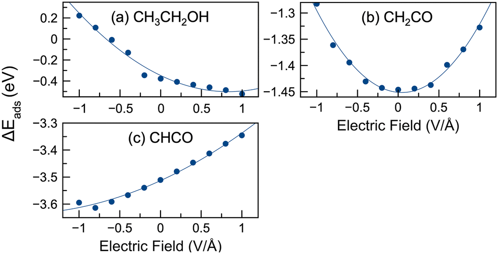 | ||
| Fig. 3 Adsorption energies of select species in the presence of electric fields. All calculations were for lone adsorbates (no water present). Three different adsorption curve patterns were observed in this work. Shown is an example of (a) negative slope (ethanol), (b) parabolic shape (CH2CO), and (c) positive slope (CHCO). | ||
Upon applying the electric fields, the optimized geometries of the adsorbates underwent only minor changes, with an example shown in Fig. S5 (ESI†). Changes in bond lengths within the adsorbates were less than 0.04 Å for all species studied when applying the electric field. In addition, we evaluated the structural fluxionality of these adsorbates following a similar approach discussed by Yang et al.,97 as described in the ESI.† This approach facilitated the comparison of adsorbate/surface geometries under electric fields with those without electric fields. The calculated structural fluxionality values, shown in Table S2 (ESI†), revealed negligible changes in geometry due to the electric fields. For example, the highest observed fluxionality value was only 0.02 Å for CH2OH at an electric field strength of 1 V Å−1.
In our study, we have investigated the variations of adsorbate–surface distances under different electrical potentials. Most of the adsorbates studied, such as CH3CH2OH, CH3CH2O, CH2CH2O, CH2OH, CH2O, CH2O, CH2O, CH2O, CH2O, CH2O, CH2O, CH2O, CH3CO, CH2CO, CH3, and OH, bonded to the surface mainly through Rh–O and Rh–C interactions. Our results showed that positive electric fields generally decreased the distances between these adsorbates and the surface, with Rh–O and Rh–C bond lengths shortened by up to 0.20 Å. Conversely, negative electric fields increased the distances. This phenomenon can be attributed to the polarization of the metal surfaces in a positive electric field, which induces a partial positive charge, increasing the attraction to negatively charged O atoms via electrostatic forces, as supported by the literature.30,41 Notably, CHCO and CO species also adsorbed through Rh–C bonds, while showing minimal distance reduction (0.03 Å) under negative potentials. In contrast, the distances for adsorbed CH2, CH and H atoms remained relatively unchanged, with bond length variations of only up to 0.01 Å. Thus, the most significant distance changes occurred for negatively charged adsorbates such as O at positive potentials, while other adsorbate distances were less affected by the applied potentials. Our results are consistent with previous studies. For example, the H adsorption energies, which increase at both positive and negative potentials, agree with the results of Che et al.40 on their investigations involving Ni(111) surfaces. This congruence extends to other species in their work as well; the adsorption energy profile of CH shows a parabolic shape, reaching optimal stability at a modest positive potential. In contrast, the adsorption energies for CH2 and CH3 show a monotonic decrease with increasing potential. The adsorption energy of CO, on the other hand, shows an upward trend with increasing potential, a trend that is also in good agreement with the findings of Che et al.,41 further validating our results by aligning with the established literature.
Fig. 3 illustrates the possible significant influence of an external electric field on the adsorption energies of reactive intermediates. The difference in adsorption energies between 1 V Å−1 and −1 V Å−1 reached up to 1 eV, with an average variation across these species of 0.44 eV. Our study also investigated the variation of adsorption energies under different potentials compared to the baseline (0 V Å−1), denoted as |E(0)ads| − |E(![[F with combining right harpoon above (vector)]](https://www.rsc.org/images/entities/i_char_0046_20d1.gif) )ads|. The maximum variance was observed for ethanol, with a value of 0.60 eV at −1 V Å−1. In Fig. 3 the largest deviations were typically observed at −1 or 1 V Å−1. The average maximum variance for all species was 0.29 eV. Some species showed significant deviations from 0 V Å−1 (e.g. ethanol, CH3CH2O, CH3COOH, OH), while others have smaller deviations (e.g. CH2CO, CHCO, CH2). For example, the adsorption energy range of CH2CO was 0.16 eV, suggesting a more limited influence of the electric potential on its adsorption.
)ads|. The maximum variance was observed for ethanol, with a value of 0.60 eV at −1 V Å−1. In Fig. 3 the largest deviations were typically observed at −1 or 1 V Å−1. The average maximum variance for all species was 0.29 eV. Some species showed significant deviations from 0 V Å−1 (e.g. ethanol, CH3CH2O, CH3COOH, OH), while others have smaller deviations (e.g. CH2CO, CHCO, CH2). For example, the adsorption energy range of CH2CO was 0.16 eV, suggesting a more limited influence of the electric potential on its adsorption.
In general, the application of a positive electric field resulted in a decrease of the adsorption energies for most of the intermediates. However, exceptions were observed for CH2CO, CH2O, CHCO, CH, CO, and H, where the adsorption energies increased in positive electric fields. This suggests that positive electric fields can stabilize many species on the surface, whereas negative fields tend to destabilize them. The implications of these field effects on the reaction energies of the steps involved in EOR are discussed later in the paper.
3.2 Dipole moments and polarizability analysis
As discussed in previous studies,30,40,41,82,98,99 dipole moments and polarizabilities can be derived from the relationship between adsorption energies and the magnitude of the local electric field. If we know the effective dipole moment and the effective polarizability, we can predict how electric field vectors with the dipole moments affect the adsorption energy of adsorbates on metal surfaces at several different potentials. The adsorption energies can be written in terms of a Taylor series expansion: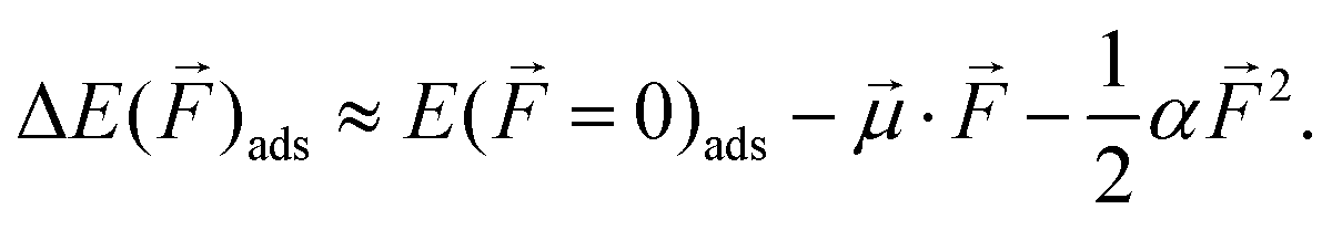 | (5) |
= 0)ads is the adsorption energy in the absence of the electric field. ![[small mu, Greek, vector]](https://www.rsc.org/images/entities/i_char_e0e9.gif) and α are defined as the effective dipole moment and polarizability evaluated at the zero electric field and can be fitted from the data. The values of and α are also the first and second derivatives of the field-dependent adsorption energies and are listed in Table 1. Fig. 3 shows the effects of electric fields on the adsorption energies of different species discussed in Section 3.1. The first group of species (CH3CH2OH, CH3CH2O, CH2CH2O, CH2OH, CH3CO, CH3, CH2, CH3COOH, and OH) experience an increase in adsorption energy under negative electric fields and a decrease under positive electric fields, which correlates with their positive effective dipole moments as listed in Table 1. Conversely, species such as CHCO and CO, which have negative effective dipole moments, show increased adsorption energies with increasing electric field strength. For CH2O and CH, which have small positive effective dipole moments (<0.1 eV Å V−1), the adsorption energies increase for both strong negative and strong positive electric fields, but decrease for weak positive fields. Similarly, for species such as CH2CO and H with near-zero effective dipole moments, both negative and positive electric fields increase their adsorption energies. These results confirm that the effect of electric fields on adsorption energies is significantly influenced by the magnitude of the effective dipole moments of the species, with pronounced field effects corresponding to stronger effective dipole moments.41 The calculated results presented in Table 1 are in agreement with previous research41 on species such as CH2OH, CH2O, CH3, CH2, CH, CO, H, and OH. This previous research focused on Ni(111) surfaces, which may explain any observed differences between our results and theirs.
and α are defined as the effective dipole moment and polarizability evaluated at the zero electric field and can be fitted from the data. The values of and α are also the first and second derivatives of the field-dependent adsorption energies and are listed in Table 1. Fig. 3 shows the effects of electric fields on the adsorption energies of different species discussed in Section 3.1. The first group of species (CH3CH2OH, CH3CH2O, CH2CH2O, CH2OH, CH3CO, CH3, CH2, CH3COOH, and OH) experience an increase in adsorption energy under negative electric fields and a decrease under positive electric fields, which correlates with their positive effective dipole moments as listed in Table 1. Conversely, species such as CHCO and CO, which have negative effective dipole moments, show increased adsorption energies with increasing electric field strength. For CH2O and CH, which have small positive effective dipole moments (<0.1 eV Å V−1), the adsorption energies increase for both strong negative and strong positive electric fields, but decrease for weak positive fields. Similarly, for species such as CH2CO and H with near-zero effective dipole moments, both negative and positive electric fields increase their adsorption energies. These results confirm that the effect of electric fields on adsorption energies is significantly influenced by the magnitude of the effective dipole moments of the species, with pronounced field effects corresponding to stronger effective dipole moments.41 The calculated results presented in Table 1 are in agreement with previous research41 on species such as CH2OH, CH2O, CH3, CH2, CH, CO, H, and OH. This previous research focused on Ni(111) surfaces, which may explain any observed differences between our results and theirs.
| This work | Literature | |||
|---|---|---|---|---|
| || |
α | || |
α | |
| *CH3CH2OH | 0.37 | −0.44 | ||
| *CH3CH2O | 0.33 | −0.17 | ||
| *CH2CH2O | 0.20 | −0.18 | ||
| *CH2OH | 0.22 | −0.03 | 0.1641 | −0.9341 |
| *CH2O | 0.09 | −0.16 | 0.3041 | 0.0041 |
| *CH3CO | 0.23 | −0.14 | ||
| *CH2CO | 0.01 | −0.29 | ||
| *CHCO | −0.14 | −0.08 | ||
| *CH3 | 0.19 | −0.11 | 0.19;41 0.1940 | −0.02;41 −0.1540 |
| *CH2 | 0.13 | −0.12 | 0.14;41 0.1440 | −0.02;41 −0.1640 |
| *CH | 0.08 | −0.19 | 0.08;41 0.0840 | −0.19;41 −0.1940 |
| *CO | −0.22 | −0.09 | −0.2141 | −0.0641 |
| *H | −0.01 | −0.06 | −0.01;41 −0.0140 | −0.03;41 −0.0640 |
| *CH3COOH | 0.47 | −0.05 | ||
| *OH | 0.56 | 0.00 | −0.0941 | −0.0541 |
3.3 Bader charge analysis
We also performed Bader charge analysis, summarized in Table 2 and illustrated in Fig. S6 (ESI†). This analysis focused on species under vacuum in order to elucidate more details how fields change adsorbate properties. It was observed that Bader charges generally decreased with increasing electric field, which was consistent with trends observed in previous studies on the Ni surface.41 The first set of species identified in Section 3.1 (including CH3CH2OH, CH3CH2O, CH2CH2O, CH2OH, CH3CO, CH3, CH2, CH3COOH, and OH) showed consistent trends in their adsorption energies. In particular, negative electric fields were found to weaken the adsorption, while positive electric fields enhanced it. These trends in adsorption energies were correlated with Bader charges. As shown in Fig. S6 (ESI†), Rh atoms bound to these intermediates were predominantly positively charged (except for CH3COOH and OH), and their charges increased as the electric field shifted from negative to positive. This increase in positive charge on Rh atoms increased their attraction to the negatively charged C and O atoms in the adsorbed species, resulting in stronger adsorption under positive electric fields. For CH3COOH, adsorption occurred through the O–Rh interaction, with both O and Rh atoms initially negatively charged. Therefore, adsorption became stronger as Rh atoms became less negatively charged under positive electric fields. Similarly, OH adsorption on Rh surfaces involves O–Rh bonding, where O atoms were negatively charged, and Rh atoms became more positively charged under positive electric fields, thus strengthening a O–Rh interaction.| Species | Vacuum | Solvation method 1 | Solvation method 2 |
|---|---|---|---|
| *CH3CH2OH | −0.15/0.03/0.04 | −0.05/0.00/−0.01 | 0.40/−0.03/0.00 |
| *CH3CH2O | −0.59/−0.40/−0.38 | −0.69/−0.46/−0.45 | −0.68/−0.43/−0.49 |
| *CH2CH2O | −0.71/−0.51/−0.36 | −0.81/−0.63/−0.53 | −0.71/−0.57/−0.73 |
| *CH2OH | −0.24/−0.06/0.06 | −0.28/−0.13/−0.04 | −0.34/−0.13/−0.14 |
| *CH2O | −0.58/−0.40/−0.27 | −0.49/−0.46/−0.36 | −0.94/−0.52/−0.41 |
| *CH3CO | −0.37/−0.17/−0.09 | −0.44/−0.28/−0.24 | −0.54/−0.28/−0.35 |
| *CH2CO | −0.60/−0.40/−0.24 | −0.71/−0.55/−0.41 | −0.87/−0.55/−0.66 |
| *CHCO | −0.47/−0.31/−0.13 | −0.63/−0.50/−0.35 | −0.69/−0.50/−0.84 |
| *CH3 | −0.35/−0.18/−0.09 | −0.22/−0.20/−0.12 | −0.52/−0.20/−0.09 |
| *CH2 | −0.44/−0.27/−0.18 | −0.30/−0.27/−0.21 | −0.78/−0.27/−0.71 |
| *CH | −0.42/−0.27/−0.20 | −0.30/−0.32/−0.26 | −1.48/−0.32/−0.23 |
| *CO | −0.42/−0.30/−0.20 | −0.51/−0.43/−0.34 | −0.63/−0.43/−0.15 |
| *H | −0.25/−0.16/−0.14 | −0.17/−0.18/−0.16 | −0.19/−0.18/−0.15 |
| *CH3COOH | −0.21/0.00/0.02 | −0.11/−0.08/−0.07 | −0.60/−0.07/−0.31 |
| *OH | −0.63/−0.46/−0.40 | −0.55/−0.48/−0.44 | −0.59/−0.48/−0.47 |
We show in Fig. S7 (ESI†) a comparison of the adsorption energies and Bader charges of Rh atoms, which illustrates how adsorption energies of species bonding through negative atoms become stronger as Rh atoms become more positively charged. For species with positive effective dipole moments (such as CH3CH2OH, CH3CH2O, CH2CH2O, CH2OH, CH3CO, CH3, CH2, CH3COOH, and OH) negative electric fields weaken adsorption, while positive fields strengthen adsorption. Because more positive charges on Rh atoms (under positive fields) increases their attraction to negatively charged C and O atoms, adsorption is strengthened. Similarly, less positive charges (under negative fields) weaken adsorption. Species with negative effective dipole moments, such as CHCO and CO, show weaker binding under positive electric fields due to increased positive charge on both Rh and C atoms, resulting in decreased adsorption. For species with small effective dipole moments, such as CH2CO, CH, and H, there is a more complex relationship between Rh charges and charges of the adsorbate.
The second group of species, CHCO and CO, was found to adsorb onto the Rh surfaces via interactions involving both C atoms in CHCO and the C atom in CO, forming Rh–C bonds. The Rh atoms in these interactions were positively charged. In CHCO, one of the carbon atoms was positively charged and the other was negatively charged, as shown in Fig. S6 (ESI†). As the electric fields shift from negative to positive, the positively charged carbon atoms in CHCO became more positively charged, while the negatively charged carbon atoms became less negatively charged. This change results in increased repulsion or decreased attraction between the Rh and carbon atoms, leading to weaker adsorption in positive electric fields. Similarly, CO molecules bonded to the Rh surface through C–Rh bonds, where both the Rh and carbon atoms were positively charged. Therefore, in positive electric fields, the repulsion or weaker bonding between the Rh and carbon atoms was increased, reducing the strength of the adsorption. Indeed, Fig. S7 (ESI†) again shows that for these species more positive Rh atoms correlates with weaker adsorption.
The third set of species, including CH2O, CH2CO, CH and H, showed adsorption characteristics different from the previous two groups, having parabolic adsorption curves (see Fig. 3 and Fig. S4, ESI†). CH2O and CH species bound to the surface through Rh–O and Rh–C bonds, respectively, while CH and H bound through Rh–C and Rh–H bonds, respectively. In CH2O and CH2CO, O atoms were negatively charged while carbon atoms were positively charged. Rh atoms bound to CH2O and CH2CO were positively charged. In positive electric fields, the charges on the oxygen atoms decreased, reducing the attraction between the negatively charged oxygen and the positively charged Rh. Conversely, in negative fields, the Rh atoms bound to oxygen became less positively charged, weakening the Rh–O bond. Thus, electric fields modulated the charges and interactions between oxygen and Rh atoms, affecting the adsorption energy profiles of CH2O and CH2CO. For CH, the carbon atom exhibited reduced negative charge in both negative and positive fields. This weakened the interaction between negatively charged carbon and positively charged Rh as reflected in the adsorption energy behavior of CH. Adsorbed H atoms were always negative upon adsorption, and in negative fields, negatively charged Rh atoms decrease the Rh–H interaction, while in positive fields, despite Rh being more positively charged, the reduced charge on H led to weaker adsorption. We note that similar negative charges for H interacting with metals were observed by others.100–102 Overall, the Bader charge analysis elucidates how external electric fields significantly influence charge transfer and ionic interactions between adsorbates and metal surfaces, altering the adsorption behavior of various intermediates.
3.4 Effect of an electric field on reactivity
Our results also show that an electric field can affect the cleavage of C–C/C–H bonds in species relevant to EOR. Calculated reaction energies for C–C bond cleavage reactions are shown in Fig. 4. There are several interesting trends. Some reaction curves were parabolic (i.e. CH3CH2OH, CH3CH2O, CH2CH2O, CHCO), while others were more linear (i.e. CH3CO and CH2CO). The application of negative electric fields was found to facilitate C–C bond dissociation by reducing the reaction energies in CH3CO, CH2CO, and, to a lesser extent, CH3CH2O. In contrast, the addition of positive electric fields resulted in increased reaction energies in most of the C–C bond cleavage reactions studied, although with a slight reduction in the case of CH3CH2OH. This phenomenon of increased reaction energies under positive electric fields could be attributed to increased adsorption energies of the reactant species (i.e., more stable reactants) and/or decreased adsorption energies of product species (i.e., less stable products), as discussed in the previous section. We do note, however, that the changes in reaction energies across the different potentials are mostly small, typically less than 0.1 eV. Exceptions are CH CO and CH2CO, where the reaction energies vary by 0.5 eV (CH3CO) and 0.25 eV (CH2CO) from −1 to 1 V Å−1. Of note, CHxCO species are generally the most favorable for C–C scission, and therefore key reaction species.76,77,103–105 Thus, an electric field had little effect on the reaction energies, except for selected species in which more negative potentials favored C–C scission.
 | ||
| Fig. 4 Reaction energies for C–C bond breaking in the presence of external electric fields in the vacuum phase. Reactions modeled: (a) CH3CH2OH → CH3 + CH2OH; (b) CH3CH2O → CH3 + CH2O; (c) CH2CH2O → CH2 + CH2O; (d) CH3CO → CH3 + CO; (e) CH2CO → CH2 + CO; (f) CHCO → CH + CO. | ||
For C–H bond cleavage, as shown in Fig. 5, both the reaction energies of CH3CO and CH2CO increased with increasing potential. The reaction energies increased by 0.37 and 0.38 eV for CH3CO and CH2CO, respectively, between −1 V Å−1 and 1 V Å−1. C–O bond formation in an electric field was more complicated. The results show that both negative and positive potentials favored C–O formation. In negative electric fields, the reaction energy decreased by up to 0.029 eV, while in positive electric fields, the reaction energy decreased by up to 0.056 eV. Thus, negative potentials favored the C–H bond cleavage and C–O bond formation reactions in EOR, while positive potentials favored only C–O bond formation. However, the effect of a potential on C–O formation was rather small.
 | ||
| Fig. 5 Reaction energies for C–H bond breaking in the presence of external electric fields in the vacuum phase, as well as C–O formation. Reactions modeled: (a) CH3CO → CH2CO + H; (b) CH2CO → CHCO + H; (c) CH3CO + OH → CH3COOH. | ||
Our results indicate that the presence of an external electric field has a significant effect on the reaction energies for selected C–C/C–H bond cleavage and C–O bond formation reactions. Negative electric fields could significantly lower the reaction energies of certain C–C and C–H bond cleavages. On the other hand, positive electric fields had minimal effect in lowering the reaction energies and significantly increased the reaction energies for some species. Both negative and positive electric fields favored the formation of the C–O bond, although the effect was small. Therefore, it appears that negative electric fields are likely to have the most beneficial effect in increasing the rate of the EOR reaction steps, at least in the absence of water. This finding correlates well with the experimental results that ethanol decomposes on Rh surfaces at negative onset potentials via C–H bond cleavage to form intermediates such as acetic acid and acetaldehyde, and C–C bond cleavage to form CO or CO2.106–109
3.5 Effect of an electric field and co-adsorbed water on adsorption
Liquid–metal interfaces occur in many electrochemical systems, such as batteries, electrolytic cells, and fuel cells.29 Therefore, in addition to electrical potentials, we also considered the effect of water on Rh surface chemistry. The inclusion of a solvent, such as water, can significantly affect surface reactions.43–45,110–112 Previous work has shown that explicit solvation methods that directly include solvent molecules as part of the simulation can accurately describe solvation effects resulting from hydrogen bonding between adsorbates and solvents.52,92,93,113–117 In our work,45 we have also shown that the inclusion of explicit water and ethanol solvent molecules can greatly affect C–C/C–H bond cleavage and C–O formation in ethanol oxidation reactions, more so than implicit solvation approaches. Explicit water–metal interfaces in the presence of external electric fields have also been studied in previous work.39,55,58 In our work, we modeled surfaces where an additional water molecule was added to the system. A similar approach of using a water molecule as a proxy for the solvent has been used previously.43,90,91 Thus, the adsorption and reaction energies in the presence of electric fields and water were calculated.In Fig. 6 we show the adsorption energies of selected species in the presence of an electric field and water. Fig. S10 (ESI†) shows similar adsorption energies for 15 different species. Unlike the vacuum calculations, the adsorption energy–potential plots for most species are parabolic, increasing with increasing/decreasing potential. Exceptions are CH3COOH and OH, which have negative slopes. The lowest adsorption energies do not always occur at 0 V Å−1, but can occur at weak positive potentials (CH3CH2O, CH2CH2O, CH2OH, CH3CO, and CH2) or weak negative potentials (CHCO, CO). Some species had their lowest adsorption energies near 0 V Å−1 (CH3CH2OH, CH2O, CH2CO, CH3, CH, and H). In the case of CO, a recent paper39 showed favorable interactions between water and CO at moderately negative potentials. We observed a similar effect where CO adsorption energies with water also decreased at moderate negative potentials.
 | ||
| Fig. 6 Adsorption energies of select species under an electric field and with water present. Two different approaches (Method 1 and 2 as discussed in the Methodology) were used for selecting initial geometries for the optimizations. Shown are three different types of situations: (a) Method 2 had lower energies than Method 1 (CH3CH2OH); (b) Methods 1 and 2 have almost identical energies (CHCO); or (c) Methods 1 and 2 give similar energies, but with some deviations (CH3). | ||
In this study, as discussed in Section 2, we started with different initial geometries at 0 V Å−1 and chose the most stable structures as the initial geometries for further calculations in electric fields (i.e. Method 1). When we started with several possible initial geometries and then applied an electric field (i.e. Method 2), the adsorption energies, as shown in Fig. 6, could be quite different for some species. In general, the adsorption energies using Method 2 followed a trend similar to that of Method 1, but the adsorption energies decreased by −0.04 eV on average. The highest increases and decreases in adsorption energy were 0.17 eV (CH3 at 1.0 V Å−1) and 0.35 eV (CH3CH2OH at −0.6 V Å−1), respectively. CH2O also had significantly lower adsorption energies with Method 2 compared to Method 1 by an average of 0.12 eV. Fig. 6 shows that the differences in adsorption energies between Methods 1 and 2 are often most pronounced at larger potentials (e.g. near 1 V Å−1 or −1 V Å−1): CH, OH, CH3, CH2, CH2CH2O, etc.
We discuss a specific example of how the optimization approach affects the final geometries. Fig. 7 and Section 7 of the ESI† both provide details on the geometries of CH3CH2O using Methods 1 and 2. When using both Method 1 and Method 2, the orientation of the water molecule adopts one of two configurations, either facing the surface as H-down (see Fig. 7 using Method 1 at −1 V Å−1), or lying flat as H-up (see Fig. 7 using Methods 1 and 2 at 0 V Å−1). However, it was observed that the water molecule preferred the H-down position towards the metal surface only under the influence of strong electric fields when Method 1 was applied. Conversely, in Method 2, the configurations of the water molecules were more complex, exhibiting both surface-facing and flat positions at different electric fields without following a consistent pattern. These patterns align with previous studies suggesting that varying electric fields significantly affect water molecule orientations and interactions on the metal surface.30,39,118 It is noteworthy that in the case of *CH3CH2O, the water favored an H-down orientation at −1.0 V Å−1 using Method 1. However, using Method 2, the H-up orientation was found to be the most energetically favorable at the same electric field. Conversely, at −0.4 V Å−1, the H-up orientation was preferred using Method 1, while the H-down configuration was energetically preferred using Method 2. This difference in geometric preferences can be attributed to the different approaches used in Method 2, where both H-up and H-down configurations were initially modeled for geometry optimization and energy calculations at various electric fields. Therefore, the Method 2 configurations shown in Fig. 7 represent the most energetically favorable results of these calculations.
 | ||
| Fig. 7 An example result showing how the optimization method affects the convergence of geometries. Shown are CH3CH2O structures in an electric field with water using Methods 1 (top) and 2 (bottom). Different orientations may arise, depending on the solvation approach and field strength. For instance, the H-down water orientation occurred at −1.0 V Å−1 using Method 1, while the H-up water orientation occurred at −1.0 V Å−1 using Method 2. Grey spheres represent carbon atoms, red spheres represent oxygen atoms, white spheres represent hydrogen atoms, and blue spheres represent rhodium atoms. | ||
Table 2 also shows that for the ethanol-related intermediates, Methods 1 and 2 yield similar Bader charges under positive electric fields and no electric field conditions. However, under strong negative electric fields at −1.0 V Å−1, pronounced differences in Bader charges are observed for species such as *CH3CH2OH, *CH2O, *CH2, *CH, and *CH3COOH. In these cases, Method 1 tends to favor the H-down configuration of the water molecules, while Method 2 shows a preference for the H-up configuration. This difference in water molecule orientation results in significant Bader charge discrepancies (greater than 0.45 e−) between the two methods, underscoring the influence of solvent interactions and molecular orientation on electronic properties.
Hydrogen bond distances at different potentials are also given in Table S3 (ESI†). As previously discussed, the differences in the most energetically favorable configurations of the intermediates between Method 1 and Method 2 can be substantial, especially under different external electric fields, mainly due to fluctuations in the orientation of the water molecules (either H-up or H-down). Consequently, these orientation differences affect the hydrogen bonding distances between water molecules and adsorbates. For example, in the case of CH3CH2O, the interaction between the water molecule and the adsorbate exhibits weak hydrogen bonding, with average bond distances of 2.75 Å for Method 1 and 2.50 Å for Method 2, showing notable differences in the most energetically stable configurations between the two methods (Fig. 7). Conversely, there are cases where the most energetically favorable structures remain consistent using both methods. To illustrate, we also provide examples such as CH2CH2O and CO, where the interaction between water molecules and adsorbates involves strong hydrogen bonding, with average bond distances of 1.49 Å for Method 1 and 1.46 Å for Method 2 in CH2CH2O, and 1.93 Å for Method 1 and 1.94 Å for Method 2 in CO. The most energetically stable geometries for CH2CH2O and CO are consistent between Method 1 and Method 2 (see Fig. S12 and S13, ESI†). In summary, Methods 1 and 2 may give similar geometries and energies for some species. But our results have also shown that simply using the most stable geometries from potential-free calculations (i.e., Method 1) may not yield the most stable geometries under an applied potential and that the initial geometries may strongly affect the geometry optimization. Care must be taken to ensure that the correct geometries are used for calculations with an electric field.
Fig. 3 shows the adsorption energies in vacuum, while Fig. 6 shows adsorption energies in the presence of water. We also show a comparison of adsorption energies in vacuum and water in Fig. S15 (ESI†). The adsorption energies decreased significantly in some cases in the presence of an electric field without a water molecule present, as indicated by the negative slope of the adsorption energy curves. However, the lowest adsorption energies tended to occur near 0 V Å−1 in the presence of water, while this was not the case with no water molecule present. Adsorption energies tended to increase in water compared to vacuum for several species: CH3CH2O, CH3, and CH2, CH. The largest increase in adsorption energy in water compared to vacuum occurred with CH3, having an increase of 0.46 eV at 1.0 V Å−1. The average adsorption energy increases in water versus vacuum are 0.14, 0.13, 0.08 and 0.08 eV for CH3CH2O, CH3, CH2, CH, respectively. However, the adsorption energies in water decreased compared to vacuum for several species: CH3CH2OH, CH2CH2O, CH2O, CH2CO, CHCO, CO, H, and OH. The average decreases in adsorption energy were −0.13, −0.16, −0.10, −0.12, −0.29, −0.16, −0.01, and −0.24 eV for CH3CH2OH, CH2CH2O, CH2O, CH2CO, CHCO, CO, H, and OH, respectively. The largest decrease was −0.42 eV for OH.
In conclusion, in the presence of water, the adsorption of several adsorbates could be significantly affected by an electric field. Water interactions with an adsorbate resulted in adsorption behavior that was significantly different from that in vacuum for many adsorbates. Adsorption energy curves in the presence of water tended to be parabolic, while adsorption energy curves in vacuum tended to be more linear, with positive or negative slopes. Adsorption energies decreased for some species in the presence of water (compared to vacuum calculations) due to the formation of intermolecular hydrogen bonds. Some species were destabilized with water compared to vacuum. In addition, relying solely on vacuum-optimized geometries to guide solvent calculations (Method 1) may not yield the most stable geometries at the applied potential. To ensure that the most stable geometries are obtained, several initial geometries should be considered (Method 2). This effect of water on adsorption energies can have an impact on reactivity, which will be discussed further in the next section.
3.6 Further electronic analysis
To gain deeper understanding of how electric fields affect the electronic interactions between adsorbates and the Rh surface, we also investigated the density of states (DOS) and charge difference density (CDD) for selected species from the three different groups which are identified in Sections 3.1 and 3.3. These species include CH3CH2OH (decreasing adsorption energy with increasing electric field), CHCO (increasing adsorption energy with increasing electric field), and CH2CO (adsorption energies increasing with increasing or decreasing electric field), as shown in Fig. 3. Fig. 8 details the DOS analysis for CH3CH2OH, with additional data for CH2CO and CHCO in Fig. S8 (ESI†). Under an electric field orbitals can change. For instance, Fig. 8 shows CH3CH2OH has increased hybridization with the orbitals of the Rh surface with increasing potential, as the CH3CH2OH levels shift up in energy (closer to the Fermi level). See for instance the orbital around −12 eV (as well as other orbitals) at −1 V Å−1 shift to high levels with increasing potential. In contrast, the orbitals for H2O appear to decrease with increasing electric field. In the case of CH2CO, orbitals move slightly closer to the Fermi level with increasing potential. On the other hand CHCO orbitals have a less discernible pattern. For all three molecules interactions between the water molecule and adsorbate are apparent, with such interactions missing in the vacuum calculations.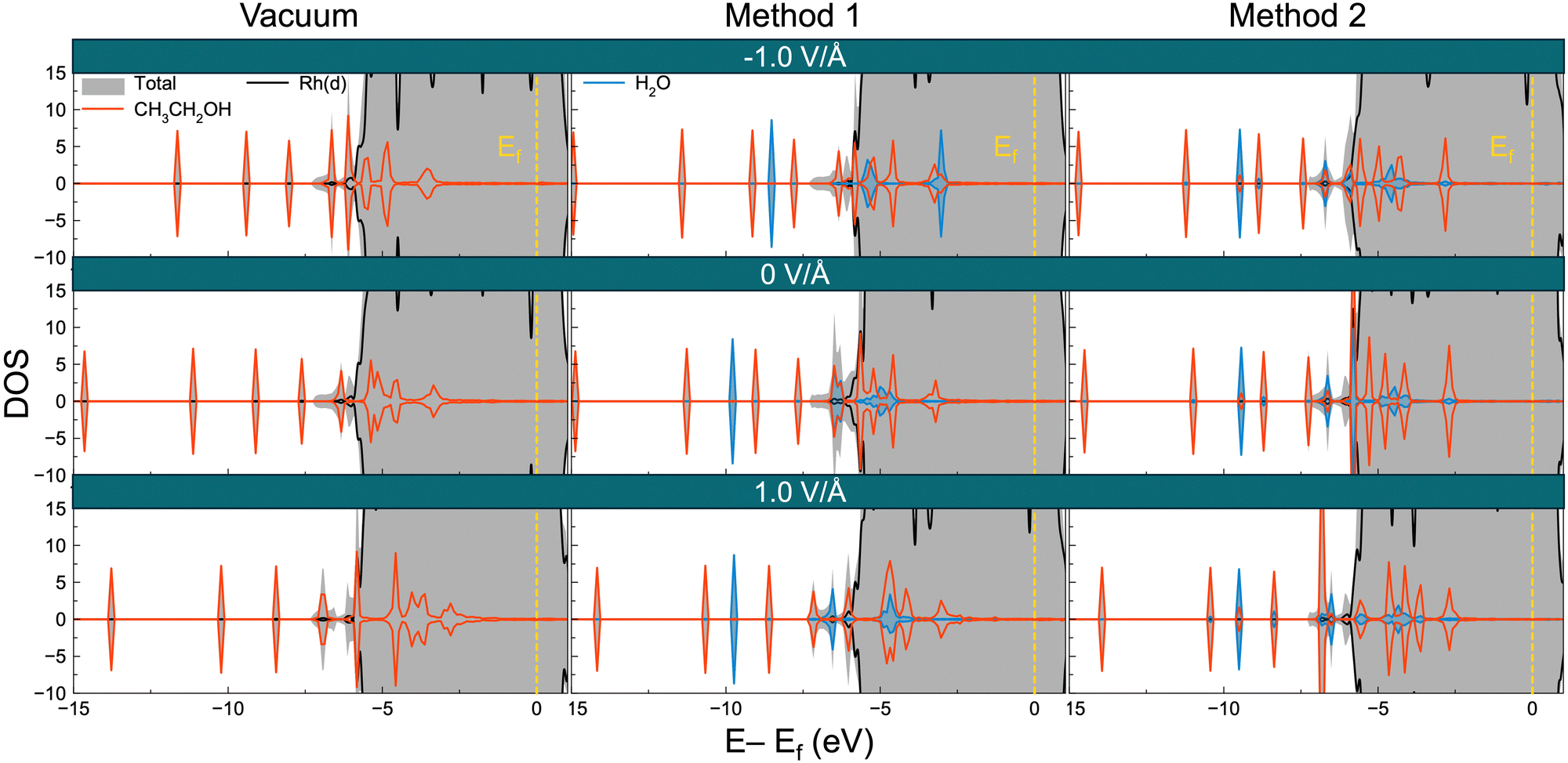 | ||
| Fig. 8 Density of states (DOS) analysis of CH3CH2OH using different solvation methods and applied fields. The figures in each row represent the DOS of the adsorbed CH3CH2OH in a negative electric field (−1 V Å−1), no electric field (0 V Å−1), and in a positive electric field (1 V Å−1). The Fermi level corresponds to 0 eV. | ||
Fig. 9 shows CDD plots for CH3CH2OH, while Fig. S9 (ESI†) shows CDD plots for CH2CO and CHCO. In vacuum CH3CH2OH has the most stable adsorption energy at positive potentials. Fig. 9 shows that in vacuum there are more electron density changes between the adsorbate and surface at 1 V Å−1, compared to the other CDD plots under vacuum, and thus is consistent with the adsorption energy behavior. Unsurprising, when water is present there are significant changes in electron density in the vicinity of the water molecule, as the water molecule interacts with both the surface and the adsorbate. Fig. 6 indicates that Method 2 geometries are the most stable for CH3CH2OH, and that adsorption energies are most stable near 0 eV, increasing under any electric field. This is consistent with the CDD plots. The CDD plots of CH3CH2OH using Method 2 have the largest electron density changes at 0 V Å−1. See for instance the region around the water molecule for these pronounced changes. Method 1 has the smallest electron density changes at −1 V Å−1, and noticeably the water molecule is farthest from the Rh surface. Similar patterns can be seen for the other molecules. CHCO, for instance, has the most stable adsorption energy in vacuum at negative potentials, and the greatest electron density changes in vacuum are seen at −1 V Å−1 for CHCO (see Fig. S9, ESI†).
 | ||
| Fig. 9 Charge density difference analysis of CH3CH2OH on the Rh(111) surface in the presence and the absence of an electric field. The yellow or blue areas represent a gain or loss of electrons. The isosurface level of the differential charge densities of CH3CH2OH is 0.004 e bohr−3. | ||
3.7 Effect of an electric field and water on reactivity
A combination of co-adsorbed water and electric field can significantly affect the surface reactions for EOR, as shown in Fig. 10 and 11. For C–C bond cleavage, the choice of initial geometries can have far-reaching effects on reaction energies. Fig. 10 shows that for many reactions Methods 1 and 2 give very different reaction-potential plots. The reaction energy plot for the C–C scission of CH3CH2OH had a parabolic shape, but the two methods give energies ∼0.3 eV apart. Interestingly, Method 2, which gives the most stable structures, had more exothermic reaction energies than Method 1. This suggests that simply using Method 1, or the most stable potential-free geometry, may underestimate C–C scission in ethanol. The plot for C–C scission of CH3CH2O was also parabolic, but the difference between the two methods was 0.04 eV on average. The plots for CH3CO and CH2CO had positive slopes, except for CH3CO using Method 2. However, the differences between Method 1 and Method 2 for the C–C cleavage of these two reactants were small, averaging 0.03 eV for CH3CO and 0.002 eV for CH2CO. An interesting phenomenon from our work shows that the reaction plots for CH2CH2O and CHCO had very different shapes depending on the initial choice of geometry for the water molecules. Method 1 gave concave parabolic curves, while Method 2 gave convex parabolic curves. This discrepancy in reaction energies between the two methods can be explained by the different geometries and adsorption behaviors of the reactants and products. For example, Fig. S14 (ESI†) illustrates the geometries for structures during C–C bond cleavage of CH2CH2O. Different final geometries of products and reactants occurred using the different solvation approaches (Methods 1 and 2). Accordingly, different reaction energy patterns emerged for CH2CH2O and CHCO. Therefore, our results again highlight the importance of the initial geometry choice, especially when multiple molecules or solvent molecule(s) may be present. | ||
| Fig. 10 Reaction energies for C–C bond breaking in the presence of an electric field and water phase. Method 1 and Method 2 were used for generating initial geometries. Reactions involved: (a) CH3CH2OH → CH3 + CH2OH; (b) CH3CH2O → CH3 + CH2O; (c) CH2CH2O → CH2 + CH2O; (d) CH3CO → CH3 + CO; (e) CH2CO → CH2 + CO; (f) CHCO → CH + CO. | ||
 | ||
| Fig. 11 Reaction energies for C–H bond breaking and C–O bond formation in the presence of an electric field and water phase. Method 1 and Method 2 were used for generating initial geometries. Reactions involved: (a) CH3CO → CH2CO + H; (b) CH2CO → CHCO + H; (c) CH3CO + OH → CH3COOH. | ||
For C–H bond cleavage (Fig. 11), the effect of an electric field was very similar for the vacuum and water cases. The reaction energies increased with increasing potential, although CH3CO showed a slight increase at very negative potentials when using Method 2. The reaction energies between Method 1 and 2 had an increase of up to 0.10 eV for the cleavage of the CH3CO C–H bond at −1.0 V Å−1, and a decrease of 0.10 eV at 1.0 V Å−1 for the cleavage of the CH2CO C–H bond. The average reaction energy changes were 0.01 eV for C–H scission in CH3CO and −0.03 eV for C–H scission in CH2CO. Methods 1 and 2 gave similar C–H scission reaction energies except at low potentials with CH3CO and high potentials with CH2CO. For C–O bond formation with water, the reaction energy curves were parabolic (concave) as in the vacuum calculations. Negative electric fields decreased the reaction energy by up to 0.30 eV, while positive electric fields decreased the reaction energy by up to 0.34 eV.
Fig. 4, 5, 10 and 11 show the reaction energies in vacuum and with water. We also show a comparison of these energies in Fig. S16 and S17 (ESI†). Comparing the reaction energies with water (Method 2) to the vacuum calculations, the reaction energies of C–C bond cleavage in CH3CH2O, CH3CO, and C–H bond cleavage in CH3CO and CH2CO were on average lower in water than in vacuum. The average energy decreases of these reactions were −0.10, −0.04, −0.14, and −0.18 eV, respectively. The largest energy decrease was −0.27 eV for the C–H bond cleavage in CH2CO. However, the reaction energies of C–C bond scission of CH3CH2OH, CH2CH2O, CH2CO, and CHCO became more endothermic in water compared to vacuum by 0.26, 0.14, 0.04, and 0.21 eV, respectively. The largest energy difference was 0.48 eV for CH3CH2OH. The C–O bond formation energies were more endothermic in water than in vacuum, with an average difference of 0.28 eV. These changes in reaction energy are due to strong adsorption of reactant intermediates (e.g., *CH2CH2O, *CH2CO) or weak adsorption of product intermediates (e.g., *CH2, *CH). The results are consistent with our previous solvation work,45 in that explicit water solvation favors C–C scission of CH3CH2O, CH3CO; and C–H scission in CH3CO and CH2CO. However, our current and previous work also showed that water inhibited the C–C scission of CH2CH2O, CH2CO and CHCO and C–O bond formation.
In summary, our results show that the application of an external electric field significantly affects the energies involved in the cleavage of C–C and C–H bonds with co-adsorbed water. This effect varies between reactions occurring under vacuum conditions and those with water, as shown in our results (as shown in Fig. 4, 5 and 10, 11). The choice of initial geometric configurations (Methods 1 and 2) yielded different results. In particular, C–C bond cleavage in molecules such as CH3CH2OH, CH3CH2O, CH3CO, along with C–H bond cleavage in CH3CO and CH2CO, showed more favorable (exothermic) reaction energies in the presence of water compared to vacuum scenarios. Conversely, certain reactions involving C–C bond cleavage (as in CH2CH2O, CH2CO, and CHCO) and C–O bond formation showed less favorable (more endothermic) results in water. In addition, the influence of electric fields on the reaction energy changes for most of the C–C bond cleavages studied typically showed a parabolic trend, with negative electric fields more likely to promote C–H bond cleavages and C–C cleavages in CH2CO. We do note that previous work46 examined C–C cleavage under potential, although only cleavage of CH3CO was studied using implicit solvation. In this work reaction energies only changed slightly with potential, possibly due to the use of implicit solvation and a different metal (Pd).
3.8 Comparing EOR reactivity in different electrochemical environments
The breaking of C–C bonds is a necessary step for the complete oxidation of ethanol. In this work, we have modeled C–C scission in three different environments: vacuum with no electric field, electric field only (vacuum), and electric field with water. We compare the reaction energies in these different environments for C–C scission in Fig. 12. We show that C–C scission is predominantly exothermic for reactions involving CHxCO (i.e., late reaction species after many C–H scission steps), whereas it is predominantly endothermic for reactions involving CH3CH2OH, CH3CH2O, and CH2CH2O (i.e., early reaction species with few C–H scission steps). This agrees with previous DFT and experimental work where CHxCO species have been implicated as key species for C–C splitting.76,77,103–105 Notably, the presence of water and an electric field does not change the fact that C–C scission is easiest through late species (CHxCO).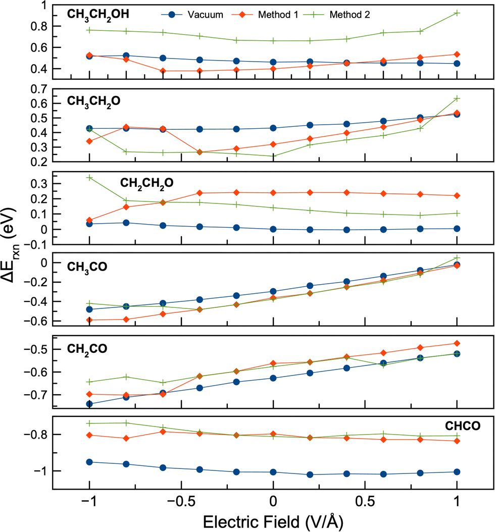 | ||
| Fig. 12 A comparison of C–C bond breaking reaction energies using the various approaches of this study. Indicated are the reactants for C–C scission, with reaction energies at different potentials. | ||
Our results show that at no applied potential (0 V Å−1), C–C scission was easiest for CHCO (i.e. the lowest reaction energy), followed by CH2CO and then CH3CO, regardless of whether water was present. The reaction energies decrease at negative potentials for CH3CO and CH2CO (positive slope), but increase for CHCO (negative slope), again regardless of whether water is present. Reaction energy changes for C–C scission of CHCO between −1 V Å−1 and 1 V Å−1 were 0.05 eV (vacuum), 0.03 eV (Method 1), and 0.07 eV (Method 2). These small numbers indicate that the applied field had only a small effect on the C–C scission of CHCO. On the other hand, the reaction energy changes for C–C scission of CH3CO between −1 V Å−1 and 1 V Å−1 were 0.46 eV (vacuum), 0.56 eV (Method 1), and 0.47 eV (Method 2). Reaction energy changes for C–C scission of CH2CO between −1 V Å−1 and 1 V Å−1 were 0.22 eV (vacuum), 0.22 eV (Method 1), and 0.12 eV (Method 2). Clearly, the electric field has a much larger effect on the scission of CH3CO and CH2CO. We note that while CHCO has the most exothermic reaction energies, at very low negative potentials the scission of CH2CO can become competitive with CHCO scission due to close reaction energies. For example, the reaction energies for CH2CO scission at −1 V Å−1 are −0.74 eV (vacuum) and −0.64 eV (Method 2), while the reaction energies for CHCO scission at −1 V Å−1 are −0.95 eV (vacuum) and −0.74 eV (Method 2). Our results thus show that negative potentials can open new reaction pathways for C–C scission involving CH2CO, and that the competition becomes more pronounced in the presence of water. This conclusion could not be reached without considering the electrochemical environment present during EOR.
We further examined the reaction data to understand and rationalize the observed trends. The reaction energy at a potential can be expanded as in the following series:119
 | (6) |
= 0)rxn is the reaction energy with no electric field applied, Δrxn is a vector of the reaction dipole moment (difference in dipole moments between products and reactants), and Δαrxn is the reaction polarizability (difference in polarizability between products and reactants). Fitting the reaction plots (Fig. 12) yields the reaction dipole moments and polarizabilities, and these values are given in Table 3. According to eqn (6), the changes in dipole moments between products and reactants (Δrxn) are the key to how much an electric field affects the reaction energies. As noted above, an electric field has little effect on the C–C cleavage of CHCO (see Fig. 12). In fact, the Δrxn values for CHCO are all small (<0.04 eV Å2 V−2), as shown in Table 3. Similarly, the difference between the product and reactant dipole moments from Table 1 for CHCO C–C scission is ≈0 eV Å2 V−2. Thus, the total change in dipole moment between products and reactants for CHCO scission is close to zero, and thus an electric field has little effect on the reaction energy for CHCO scission. This is not the case for CH2CO and CH3CO, where the changes in dipole moments (using values from Table 1 and also using data from Table 3) are all negative, indicating that an electric field would and does have a measurable effect on the reaction energies. Notably, we observe that changes in dipole moments occur regardless of whether water is present or not.
| Vacuum | Method 1 | Method 2 | ||||
|---|---|---|---|---|---|---|
| |Δrxn| |
Δαrxn | |Δrxn| |
Δαrxn | |Δrxn| |
Δαrxn | |
| *CH3CH2OH | 0.0376 | −0.0414 | −0.026 | −0.2772 | −0.0333 | −0.346 |
| *CH3CH2O | −0.0475 | −0.0878 | −0.0696 | −0.2804 | −0.1038 | −0.4754 |
| *CH2CH2O | 0.0206 | −0.0398 | −0.0602 | 0.208 | 0.0901 | −0.1394 |
| *CH3CO | −0.2314 | −0.0842 | −0.287 | −0.1164 | −0.2269 | −0.3832 |
| *CH2CO | −0.109 | 0.0076 | −0.1229 | 0.0356 | −0.063 | 0.005 |
| *CHCO | 0.0288 | −0.0672 | 0.0173 | 0.0358 | 0.0354 | −0.0786 |
We do acknowledge the limitations of our results. All our calculations have essentially been static calculations, focused on reaction energies. This approach has been used previously to study EOR.45,46 Activation energies would provide more insight into the nature of these reaction steps. However, such calculations are time-consuming and complicated, especially when incorporating solvation and electric fields. Such calculations may be the topic of future work. Scaling relationships do indicate that often activation energies are proportional to reaction energies, and linear scaling relationships have been applied to the study of C–C breaking of ethanol over various metals (albeit with no electric fields or solvent molecules present).77,103 Related work37 on methane steam reforming over Ni showed linear scaling relationships changed only slightly in the presence of both positive or negative electric fields. Thus, we expect lower reaction energies to correspond to lower activation energies. We also point out that modeling the dynamic nature of electrochemical reactions is an ongoing area of research. For instance, kinetic Monte Carlo calculations have been used to simulate electrocatalytic systems as they change over time120,121 or ethanol decomposition.76 Certainly applying such methods to study the EOR would provide valuable insights, and again may be the topic of future work.
4 Conclusions
Our results showed that electric fields significantly modify the oxidation process. Under vacuum conditions the adsorption energy differences between results using fields of 1 V Å−1 and −1 V Å−1 were up to 1 eV, with an average change of 0.44 eV. Positive electric fields generally reduced the adsorption energies for most species except CH2CO, CHCO, CO, and H atoms, while negative electric fields tended to favor the adsorption of CHCO and CO species only. Negative fields reduced reaction energies for some C–C and C–H bond cleavage reactions by up to 0.5 eV, but also enhanced C–O bond formation. Positive fields had little impact on lowering reaction energies, occasionally increasing them. These results correlate well with experimental findings that negative potentials lead to ethanol reduction. The study also aligned with previous findings that positive electric fields lower adsorption energies for species with positive dipole moments (i.e. CH3CH2OH, CH3CH2O, CH2CH2O, CH2OH, CH2O, CH3CO, CH3, CH2, and CH), while negative electric fields produce a similar effect for molecules with negative dipole moments (i.e. CHCO and CO). Additionally, for species whose dipole moments are approximately zero, adsorption energies increase in both positive and negative electric fields (i.e. CH2CO and H).We also examined how electric fields and the presence of water impact ethanol oxidation on Rh(111). We employed two methods to incorporate water molecules into our calculations. In Method 1 the initial geometries were taken from converged structures involving no electric fields. In Method 2 four different initial geometries were used at each electric field strength. Method 2 is a more robust process to explore possible structures, but also more time-consuming. These approaches yielded different geometries and energy profiles for several species, emphasizing the importance of a comprehensive exploration of possible geometries in electrochemical systems. The presence of water altered the adsorption energy trends, causing them to generally become more parabolic under an electric field. It also enhanced C–C and C–H bond cleavage by up to −0.27 eV but could inhibit C–O bond formation by about 0.28 eV. Electric fields, especially negative fields, favor the cleavage of C–H and specific C–C bonds such as CH2CO, while most C–C bond cleavages become more parabolic under an electric field in the presence of water. We also found that C–C bond cleavage is most likely to occur in CHCO, followed by CH2CO and CH3CO. Although electric fields have minimal effect on C–C bond cleavage in CHCO, they significantly affect CH2CO C–C cleavage. Under strong electric fields C–C scission through CHCO and CH2CO become competitive, demonstrating the potential of electric fields to manipulate chemical reaction pathways. Overall, our study illuminates the significance of electric fields and solvent molecules in electrochemical ethanol oxidation, showcasing their impact on adsorption processes and reaction pathways.
Data availability
Data for this article are included in the main text and ESI.† Simulation files are available at: https://github.com/Deskins-group/Structure-Files/tree/master/Ethanol%20Oxidation%20-%20Potential.Conflicts of interest
There are no conflicts to declare.Acknowledgements
This work was supported by the National Science Foundation under Grant No. 1705830. We also acknowledge the computational resources provided by Worcester Polytechnic Institute.Notes and references
- S. Q. Song, W. J. Zhou, Z. H. Zhou, L. H. Jiang, G. Q. Sun, Q. Xin, V. Leontidis, S. Kontou and P. Tsiakaras, Int. J. Hydrogen Energy, 2005, 30, 995–1001 CrossRef CAS.
- Y. Wang, S. Zou and W. B. Cai, Catalysts, 2015, 5, 1507–1534 CrossRef CAS.
- F. Barbir and T. Gómez, Int. J. Hydrogen Energy, 1997, 22, 1027–1037 CrossRef CAS.
- X. Li and I. Sabir, Int. J. Hydrogen Energy, 2005, 30, 359–371 CrossRef CAS.
- A. S. Aricè, P. Cretì, P. L. Antonucci and V. Antonucci, Electrochem. Solid-State Lett., 1998, 1, 66–68 CrossRef.
- M. Z. Kamarudin, S. K. Kamarudin, M. S. Masdar and W. R. Daud, Int. J. Hydrogen Energy, 2013, 38, 9438–9453 CrossRef CAS.
- M. Li, A. Kowal, K. Sasaki, N. Marinkovic, D. Su, E. Korach, P. Liu and R. R. Adzic, Electrochim. Acta, 2010, 55, 4331–4338 CrossRef CAS.
- U. B. Demirci, J. Power Sources, 2007, 173, 11–18 CrossRef CAS.
- Y. M. Choi and P. Liu, J. Am. Chem. Soc., 2009, 131, 13054–13061 CrossRef CAS PubMed.
- M. Li, W. Guo, R. Jiang, L. Zhao, X. Lu, H. Zhu, D. Fu and H. Shan, J. Phys. Chem. C, 2010, 114, 21493–21503 CrossRef CAS.
- R. Jiang, W. Guo, M. Li, H. Zhu, L. Zhao, X. Lu and H. Shan, J. Mol. Catal. A: Chem., 2011, 344, 99–110 CrossRef CAS.
- J. Bai, D. Liu, J. Yang and Y. Chen, ChemSusChem, 2019, 12, 2117–2132 CrossRef CAS PubMed.
- L. Yaqoob, T. Noor and N. Iqbal, RSC Adv., 2021, 11, 16768–16804 RSC.
- K. Schwarz and R. Sundararaman, Surf. Sci. Rep., 2020, 75, 100492 CrossRef CAS PubMed.
- R. Sundararaman, D. Vigil-Fowler and K. Schwarz, Chem. Rev., 2022, 122, 10651–10674 CrossRef CAS PubMed.
- J. A. Herron, Y. Morikawa and M. Mavrikakis, Proc. Natl. Acad. Sci. U. S. A., 2016, 113, E4937–E4945 CrossRef CAS PubMed.
- A. A. Peterson, F. Abild-Pedersen, F. Studt, J. Rossmeisl and J. K. Nørskov, Energy Environ. Sci., 2010, 3, 1311–1315 RSC.
- J. Cheng and M. Sprik, Phys. Chem. Chem. Phys., 2012, 14, 11245–11267 RSC.
- J. Cheng, X. Liu, J. VandeVondele, M. Sulpizi and M. Sprik, Acc. Chem. Res., 2014, 47, 3522–3529 CrossRef CAS.
- X. Zhao and Y. Liu, J. Am. Chem. Soc., 2021, 143, 9423–9428 CrossRef CAS PubMed.
- S. Yu, Z. Levell, Z. Jiang, X. Zhao and Y. Liu, J. Am. Chem. Soc., 2023, 145, 25352–25356 CrossRef CAS PubMed.
- J. Neugebauer and M. Scheffler, Phys. Rev. B: Condens. Matter Mater. Phys., 1992, 46, 16067–16080 CrossRef CAS PubMed.
- J. Rossmeisl, J. K. Nørskov, C. D. Taylor, M. J. Janik and M. Neurock, J. Phys. Chem. B, 2006, 110, 21833–21839 CrossRef CAS.
- S. R. Kelly, C. Kirk, K. Chan and J. K. Nørskov, J. Phys. Chem. C, 2020, 124, 14581–14591 CrossRef CAS.
- C.-H. Yeh, T. M. L. Pham, S. Nachimuthu and J.-C. Jiang, ACS Catal., 2019, 9, 8230–8242 CrossRef CAS.
- X. Z. Jiang, M. Feng, W. Zeng and K. H. Luo, Proc. Combust. Inst., 2019, 37, 5525–5535 CrossRef CAS.
- X. Z. Jiang and K. H. Luo, Proc. Combust. Inst., 2021, 38, 6605–6613 CrossRef CAS.
- Y. Pan, X. Wang, W. Zhang, L. Tang, Z. Mu, C. Liu, B. Tian, M. Fei, Y. Sun and H. Su, et al. , Nat. Commun., 2022, 13, 3063 CrossRef CAS.
- F. Che, J. T. Gray, S. Ha, N. Kruse, S. L. Scott and J. S. McEwen, ACS Catal., 2018, 8, 5153–5174 CrossRef CAS.
- F. Che, J. T. Gray, S. Ha and J. S. McEwen, J. Catal., 2015, 332, 187–200 CrossRef CAS.
- G. S. Karlberg, J. Rossmeisl and J. K. Nørskov, Phys. Chem. Chem. Phys., 2007, 9, 5158–5161 RSC.
- V. V. Welborn, L. Ruiz Pestana and T. Head-Gordon, Nat. Catal., 2018, 1, 649–655 CrossRef.
- P. Besalu-Sala, M. Sola, J. M. Luis and M. Torrent-Sucarrat, ACS Catal., 2021, 11, 14467–14479 CrossRef CAS.
- Z. Zhang, C. Li, X. Du, Y. Zhu, L. Huang, K. Yang, J. Zhao, C. Liang, Q. Yu, S. Li, X. Liu and Y. Zhai, Chem. Eng. J., 2023, 452, 139098 CrossRef CAS.
- J. Haruyama, T. Ikeshoji and M. Otani, Phys. Rev. Mater., 2018, 2, 095801 CrossRef.
- K.-Y. Yeh and M. J. Janik, J. Comput. Chem., 2011, 32, 3399–3408 CrossRef CAS PubMed.
- F. Che, J. T. Gray, S. Ha and J. S. McEwen, ACS Catal., 2017, 7, 551–562 CrossRef CAS.
- J. T. Gray, F. Che, J.-S. McEwen and S. Ha, Appl. Catal., B, 2020, 260, 118132 CrossRef CAS.
- A. Estejab, R. A. García Cárcamo and R. B. Getman, Phys. Chem. Chem. Phys., 2022, 24, 4251–4261 RSC.
- F. Che, R. Zhang, A. J. Hensley, S. Ha and J. S. McEwen, Phys. Chem. Chem. Phys., 2014, 16, 2399–2410 RSC.
- F. Che, S. Ha and J.-S. McEwen, Appl. Catal., B, 2016, 195, 77–89 CrossRef CAS.
- W. Zhou, W. Zhou, L. Yang and Z. Jia, Fuel, 2023, 350, 128759 CrossRef CAS.
- B. Schweitzer, S. N. Steinmann and C. Michel, Phys. Chem. Chem. Phys., 2019, 21, 5368–5377 RSC.
- G. H. Gu, B. Schweitzer, C. Michel, S. N. Steinmann, P. Sautet and D. G. Vlachos, J. Phys. Chem. C, 2017, 121, 21510–21519 CrossRef CAS.
- Y. Mei and N. A. Deskins, Phys. Chem. Chem. Phys., 2021, 23, 16180–16192 RSC.
- Y. Guo, B. Li, S. Shen, L. Luo, G. Wang and J. Zhang, ACS Appl. Mater. Interfaces, 2021, 13, 16602–16610 CrossRef CAS.
- M. Li, A. Kowal, K. Sasaki, N. Marinkovic, D. Su, E. Korach, P. Liu and R. R. Adzic, Electrochim. Acta, 2010, 55, 4331–4338 CrossRef CAS.
- H. Idriss, Platinum Met. Rev., 2004, 48, 105–115 CrossRef CAS.
- G. Yang, A. I. Frenkel, D. Su and X. Teng, ChemCatChem, 2016, 8, 2876–2880 CrossRef CAS.
- A. Resta, J. Blomquist, J. Gustafson, H. Karhu, A. Mikkelsen, E. Lundgren, P. Uvdal and J. N. Andersen, Surf. Sci., 2006, 600, 5136–5141 CrossRef CAS.
- M. Mavrikakis, J. Rempel, J. Greeley, L. B. Hansen, J. K. Nørskov and J. Rempel, J. Chem. Phys., 2002, 117, 6730–6741 CrossRef.
- C. Michel, F. Auneau, F. Delbecq and P. Sautet, ACS Catal., 2011, 1, 1430–1440 CrossRef CAS.
- M. M. Yang, X. H. Bao and W. X. Li, J. Phys. Chem. C, 2007, 111, 7403–7410 CrossRef CAS.
- A. Y. Lozovoi, A. Alavi, J. Kohanoff and R. M. Lynden-Bell, J. Chem. Phys., 2001, 115, 1661–1669 CrossRef CAS.
- C. D. Taylor, S. A. Wasileski, J. S. Filhol and M. Neurock, Phys. Rev. B: Condens. Matter Mater. Phys., 2006, 73, 165402 CrossRef.
- A. Y. Lozovoi and A. Alavi, Phys. Rev. B: Condens. Matter Mater. Phys., 2003, 68, 245416 CrossRef.
- Y. He, X. Y. Wei, C. T. Chan and J. G. Che, Phys. Rev. B: Condens. Matter Mater. Phys., 2005, 71, 45401 CrossRef.
- J. S. Filhol and M. Neurock, Angew. Chem., Int. Ed., 2006, 45, 402–406 CrossRef CAS.
- J. K. Nørskov, J. Rossmeisl, A. Logadottir, L. Lindqvist, J. R. Kitchin, T. Bligaard and H. Jónsson, J. Phys. Chem. B, 2004, 108, 17886–17892 CrossRef.
- G. Rostamikia, A. J. Mendoza, M. A. Hickner and M. J. Janik, J. Power Sources, 2011, 196, 9228–9237 CrossRef CAS.
- X. K. Gu and E. Nikolla, J. Phys. Chem. C, 2015, 119, 26980–26988 CrossRef CAS.
- H.-F. Wang and Z.-P. Liu, J. Phys. Chem. C, 2009, 113, 17502–17508 CrossRef CAS.
- J. R. Pliego and J. M. Riveros, J. Phys. Chem. A, 2001, 105, 7241–7247 CrossRef CAS.
- G. Kresse and J. Hafner, Phys. Rev. B: Condens. Matter Mater. Phys., 1994, 49, 14251–14269 CrossRef CAS.
- G. Kresse and J. Hafner, Phys. Rev. B: Condens. Matter Mater. Phys., 1993, 47, 558–561 CrossRef CAS.
- G. Kresse and J. Furthmüller, Phys. Rev. B: Condens. Matter Mater. Phys., 1996, 54, 11169–11186 CrossRef CAS.
- G. Kresse and J. Furthmüller, Comput. Mater. Sci., 1996, 6, 15–50 CrossRef CAS.
- P. E. Blöchl, Phys. Rev. B: Condens. Matter Mater. Phys., 1994, 50, 17953–17979 CrossRef.
- G. Kresse and D. Joubert, Phys. Rev. B: Condens. Matter Mater. Phys., 1999, 59, 1758–1775 CrossRef CAS.
- J. P. Perdew, K. Burke and M. Ernzerhof, Phys. Rev. Lett., 1996, 77, 3865–3868 CrossRef CAS.
- M. Methfessel and A. T. Paxton, Phys. Rev. B: Condens. Matter Mater. Phys., 1989, 40, 3616–3621 CrossRef CAS PubMed.
- G. Henkelman, A. Arnaldsson and H. Jónsson, Comput. Mater. Sci., 2006, 36, 354–360 CrossRef.
- E. Sanville, S. D. Kenny, R. Smith and G. Henkelman, J. Comput. Chem., 2007, 28, 899–908 CrossRef CAS PubMed.
- W. Tang, E. Sanville and G. Henkelman, J. Phys.: Condens. Matter, 2009, 21, 84204 CrossRef CAS.
- M. L. Williams, Occup. Environ. Med., 1996, 53, 504 CrossRef.
- Y. Choi and P. Liu, Catal. Today, 2011, 165, 64–70 CrossRef CAS.
- P. Ferrin, D. Simonetti, S. Kandoi, E. Kunkes, J. A. Dumesic, J. K. Nørskov and M. Mavrikakis, J. Am. Chem. Soc., 2009, 131, 5809–5815 CrossRef CAS PubMed.
- H.-F. Wang and Z.-P. Liu, J. Am. Chem. Soc., 2008, 130, 10996–11004 CrossRef CAS PubMed.
- Q. Meng, Y. Shen, J. Xu and J. Gong, Chin. J. Catal., 2012, 33, 407–415 CrossRef CAS.
- M. Shetty, M. A. Ardagh, Y. Pang, O. A. Abdelrahman and P. J. Dauenhauer, ACS Catal., 2020, 10, 12867–12880 CrossRef CAS.
- A. Alizadeh Sahraei and F. Larachi, Appl. Surf. Sci., 2021, 576, 151899 CrossRef.
- P. Deshlahra, E. E. Wolf and W. F. Schneider, J. Phys. Chem. A, 2009, 113, 4125–4133 CrossRef CAS PubMed.
- P. J. Feibelman, Phys. Rev. B: Condens. Matter Mater. Phys., 2001, 64, 125403 CrossRef.
- R. Alcalá, M. Mavrikakis and J. A. Dumesic, J. Catal., 2003, 218, 178–190 CrossRef.
- F. Colmati, G. Tremiliosi-Filho, E. R. Gonzalez, A. Berná, E. Herrero and J. M. Feliu, Phys. Chem. Chem. Phys., 2009, 11, 9114–9123 RSC.
- B. Miao, Z.-P. Wu, H. Xu, M. Zhang, Y. Chen and L. Wang, Comput. Mater. Sci., 2019, 156, 175–186 CrossRef CAS.
- B. Miao, Z. Wu, H. Xu, M. Zhang, Y. Chen and L. Wang, Chem. Phys. Lett., 2017, 688, 92–97 CrossRef CAS.
- E. A. Monyoncho, S. N. Steinmann, P. Sautet, E. A. Baranova and C. Michel, Electrochim. Acta, 2018, 274, 274–278 CrossRef CAS.
- A. O. Pereira and C. R. Miranda, Appl. Surf. Sci., 2014, 288, 564–571 CrossRef CAS.
- Q. Zhang and A. Asthagiri, Catal. Today, 2019, 323, 35–43 CrossRef CAS.
- D. Loffreda, C. Michel, F. Delbecq and P. Sautet, J. Catal., 2013, 308, 374–385 CrossRef CAS.
- C. J. Bodenschatz, S. Sarupria and R. B. Getman, J. Phys. Chem. C, 2015, 119, 13642–13651 CrossRef CAS.
- T. Xie, S. Sarupria and R. B. Getman, Mol. Simul., 2017, 43, 370–378 CrossRef CAS.
- T. Xie, C. J. Bodenschatz and R. B. Getman, React. Chem. Eng., 2019, 4, 383–392 RSC.
- X. Zhang, R. S. DeFever, S. Sarupria and R. B. Getman, J. Chem. Inf. Model., 2019, 59, 2190–2198 CrossRef CAS PubMed.
- J. Zhang, X. M. Cao, P. Hu, Z. Zhong, A. Borgna and P. Wu, J. Phys. Chem. C, 2011, 115, 22429–22437 CrossRef CAS.
- C. T. Yang, B. C. Wood, V. R. Bhethanabotla and B. Joseph, Phys. Chem. Chem. Phys., 2015, 17, 25379–25392 RSC.
- J. S. Filhol and M. L. Doublet, J. Phys. Chem. C, 2014, 118, 19023–19031 CrossRef CAS.
- E. Masumian, S. M. Hashemianzadeh and A. Nowroozi, Phys. Lett. Sect. A: Gen. At. Solid State Phy.s, 2014, 378, 2549–2552 CrossRef CAS.
- Y. Dong, J. Dang, W. Wang, S. Yin and Y. Wang, ACS Appl. Mater. Interfaces, 2018, 10, 39624–39630 CrossRef CAS.
- S. Aboud and J. Wilcox, J. Phys. Chem. C, 2010, 114, 10978–10985 CrossRef CAS.
- G. Hu, Z. Wu and D. E. Jiang, J. Mater. Chem. A, 2018, 6, 7532–7537 RSC.
- J. E. Sutton and D. G. Vlachos, Ind. Eng. Chem. Res., 2015, 54, 4213–4225 CrossRef CAS.
- D. Cantane, W. Ambrosio, M. Chatenet and F. Lima, J. Electroanal. Chem., 2012, 681, 56–65 CrossRef CAS.
- Q. He, S. Mukerjee, B. Shyam, D. Ramaker, S. Parres-Esclapez, M. Illán-Gómez and A. Bueno-López, J. Power Sources, 2009, 193, 408–415 CrossRef CAS.
- F. Zhang, D. Zhou, Z. Zhang, M. Zhou and Q. Wang, RSC Adv., 2015, 5, 91829–91835 RSC.
- J. Zhang, J. Ye, Q. Fan, Y. Jiang, Y. Zhu, H. Li, Z. Cao, Q. Kuang, J. Cheng, J. Zheng and Z. Xie, J. Am. Chem. Soc., 2018, 140, 11232–11240 CrossRef CAS.
- H. Li, J. Ye, X. Li, J. Zhang, Y. Zhu, Z. Zhou, Y. Xue, Y. Jiang, Z. Xie and L. Zheng, J. Mater. Chem. A, 2019, 7, 26266–26271 RSC.
- G. Yang, L. Farsi, Y. Mei, X. Xu, A. Li, N. A. Deskins and X. Teng, J. Am. Chem. Soc., 2019, 141, 9444–9447 CrossRef CAS.
- J. J. Varghese and S. H. Mushrif, React. Chem. Eng., 2019, 4, 165–206 RSC.
- M. Saleheen and A. Heyden, ACS Catal., 2018, 8, 2188–2194 CrossRef CAS.
- C. D. Taylor and M. Neurock, Curr. Opin. Solid State Mater. Sci., 2005, 9, 49–65 CrossRef CAS.
- B. N. Zope, D. D. Hibbitts, M. Neurock and R. J. Davis, Science, 2010, 330, 74–78 CrossRef CAS PubMed.
- C. Hartnig, J. Grimminger and E. Spohr, Electrochim. Acta, 2007, 52, 2236–2243 CrossRef CAS.
- M. Faheem and A. Heyden, J. Chem. Theory Comput., 2014, 10, 3354–3368 CrossRef CAS.
- H. H. Heenen, J. A. Gauthier, H. H. Kristoffersen, T. Ludwig and K. Chan, J. Chem. Phys., 2020, 152, 144703 CrossRef CAS PubMed.
- J. A. Herron, Y. Morikawa and M. Mavrikakis, Proc. Natl. Acad. Sci. U. S. A., 2016, 113, E4937–E4945 CrossRef CAS.
- J.-S. Filhol and M.-L. Bocquet, Chem. Phys. Lett., 2007, 438, 203–207 CrossRef CAS.
- M. Wan, H. Yue, J. Notarangelo, H. Liu and F. Che, JACS Au, 2022, 2, 1338–1349 CrossRef CAS.
- C. H. Lee, S. Pahari, N. Sitapure, M. A. Barteau and J. S.-I. Kwon, ACS Catal., 2023, 13, 8336–8346 CrossRef CAS.
- Y. Luo, Y. Guan, G. Liu, Y. Wang, J. Li and L. Ricardez-Sandoval, ACS Catal., 2024, 14, 2696–2708 CrossRef CAS.
Footnote |
| † Electronic supplementary information (ESI) available. See DOI: https://doi.org/10.1039/d4cp02765e |
| This journal is © the Owner Societies 2024 |