A multiphoton ionisation photoelectron imaging study of thiophene

Abstract

Thiophene is a prototype for the excited state photophysics that lies at the heart of many technologies within the field of organic electronics. Here, we report a multiphoton ionisation photoelectron imaging study of gas-phase thiophene using a range of photon energies to excite transitions from the ground electronic state to the first two electronically excited singlet states, from the onset of absorption to the absorption maximum. Analysis of the photoelectron spectra and angular distributions reveal features arising from direct photoionisation from the ground electronic state, and resonance-enhanced photoionisation via the electronically excited singlet states. The first two ionisation energies from the ground electronic state were confirmed to be 8.8 eV (adiabatic) and 9.6 eV (vertical). The ionisation energies from the first two electronically excited singlet states were found to be 3.7 eV (adiabatic) and 4.4 eV (vertical).

---

1 Introduction

Thiophene is a small, heteroaromatic molecule that is a ubiquitous building block in many photonic materials, such as organic photovoltaics^1–3 and non-linear optical devices.^4,5 Although there have been many attempts to elucidate both the electronic structure and the excited-state dynamics of gas-phase thiophene,^6–33 its UV photoabsorption and photoionisation are still not understood fully.

One of the difficulties in understanding the photoabsorption spectrum arises as a result of the first two electronically excited singlet states, S₁ (ππ*) and S₂ (ππ*), hereafter referred to as S₁ and S₂, lying very close together in energy and having similar oscillator strengths. Theoretical studies by Holland et al.²⁶ and Prlj et al.²⁹ have highlighted how the precise energies and ordering of these states are highly dependent on the method and the basis sets used. Although there is still not a clear consensus on the origin of structure in the UV photoabsorption of thiophene, all assignments reported in the literature do agree that the intense feature at 5.157 eV is the origin of S₁^{6,8,10,11,13,14,17,22,26,33} (Fig. 1), with the peaks below the origin being variously attributed to hot bands, combination bands, or vibronic coupling between S₁ and S₂.^8,11,13

Fig. 1 Left: Photoabsorption spectrum of thiophene recorded by Holland et al.²⁶ Right: Schematic energy level diagram for thiophene showing the vertical excitation energies of S₁, S₂, and S₃, and the vertical ionisation energies to D₀ and D₁ continua. The adiabatic excitation energy (AEE) for S₁ is taken from measurements by Holland et al.,²⁶ vertical excitation energies (VEE) for S₁ and S₂ are taken from magnetic circular dichroism measurements from Hakansson et al.,³⁴ the AEE of S₂ is taken from DFT/MRCI calculations by Salzmann et al.,²³ the S₃ VEE is from Holland et al.²⁶ The ionisation energies D₀ and D₁ are taken from Weinkauf et al.²² The coloured arrows signify the different wavelengths used for one-colour measurements in the work reported here.

There have been two recent vacuum ultraviolet (VUV) absorption spectroscopy studies of gas-phase thiophene.^26,33 Both measurements found several progressions which were assigned to the ν₆ vibrational mode, corresponding to a CH in-plane bending vibration, with an average peak spacing of ∼120 meV. This supported earlier work by Palmer et al.,¹⁷ in which the 0–0 transition was determined to be 5.157 eV, and structure below this transition was ascribed to hot bands and S₁–S₂ vibronic coupling.

Another way to probe electronic structure is to use photoelectron spectroscopy to determine electron binding energies, eBE = hν − eKE, where hν is the photon energy and eKE is the measured electron kinetic energy. Ionisation energies of thiophene determined from such measurements are presented in Table 1. Measuring the photoelectron angular distribution (PAD) as well as the eKE provides additional information about the molecular orbital from which the electron is removed. For a two-photon ionisation process, the angular distribution I(θ) ∝ 1 + β₂P₂(cos θ) + β₄P₄(cos θ), where I(θ) is the probability of photoelectron emission at angle θ, defined as the angle between the laser polarisation and the velocity vector of the photoelectron, β₂ and β₄ are the photoelectron anisotropy parameters, and P₂(cos θ) and P₄(cos θ) are the second and fourth-order Legendre polynomials in cos θ.³⁵ The two limiting values of β₂ are +2 and −1, corresponding to photoelectron emission predominantly parallel and perpendicular to the electric field vector of the laser, respectively. β₄ represents the alignment of the excited state and, generally, positive and negative values of β₄ correspond to the excited state being aligned parallel or perpendicular to the electric field vector of the laser, respectively.

Table 1 S₀–D₀ and S₀–D₁ vertical ionisation energies (VIEs) and adiabatic ionisation energies (AIEs), in eV, recorded using a range of ionisation and PES methods: ionisation using HeI or Ly-α radiation with a hemispherical electron energy analyser (HEA); Penning ionisation electron spectra (PIES) with He* (2³S) and a hemispherical analyser; zero-kinetic energy (ZEKE) PES; time-resolved 1 + 1′ PES (TRPES) with a magnetic bottle time-of-flight (TOF) (pump–probe delay = 50 fs); femtosecond 1 + 1 multiphoton ionisation (MPI) with velocity-map imaging (VMI)

D0	AIE/VIE	D1	AIE/VIE	Method	Ref.
a Adiabatic and vertical ionisation energies not distinguished.
8.87 ± 0.05	AIE^a	9.49 ± 0.1	VIE	HeI + HEA	Eland^36
8.80 ± 0.05	AIE^a	9.44 ± 0.05	AIE^a	HeI + HEA	Baker et al.^7
8.872 ± 0.015	AIE^a	9.52 ± 0.015	VIE	Ly-α + HEA	Derrick et al.^37
8.90 ± 0.015	VIE	9.50 ± 0.015	VIE	HeI + HEA	Clark et al.^9
8.85 ± 0.05	VIE	9.49 ± 0.05	VIE	HeI + HEA	Klasinc et al.^12
8.96 ± 0.25	VIE	9.58 ± 0.25	VIE	He* PIES + HEA	Kishimoto et al.^38
8.8742 ± 0.0002	AIE	—	—	ZEKE	Yang et al.^39
8.87 ± 0.01	AIE	9.55 ± 0.01	VIE	TRPES + TOF	Weinkauf et al.^22
8.8 ± 0.1	AIE	9.6 ± 0.1	VIE	MPI + VMI	This work

---

Multiphoton ionisation (MPI) photoelectron spectroscopy studies of gas-phase thiophene using UV laser pulses have been reported by two groups.^22,32 However, there has only been one photoelectron imaging study;³² this was a time-resolved study focussing on relaxation dynamics, and PADs were not reported. Here, we present a systematic one-colour MPI photoelectron imaging study of thiophene, employing wavelengths ranging from 243 nm, exciting just below the S₀–S₁ 0–0 transition, to 234 nm, which corresponds to the S₀–S₁ VEE (Fig. 1), from which we gain further insight into the electronic structure!

2. Methods

2.1. Multiphoton photoelectron imaging

A molecular beam of thiophene was produced by passing 1 bar He carrier gas through liquid thiophene and expanding it through a 300 μm pulsed Amsterdam piezovalve^40,41 operating at a repetition rate of 1 kHz and with a pulse duration of 8 μs. The molecular beam was collimated by a 3 mm skimmer before passing into the interaction region of our velocity map imaging spectrometer that has been described before.^42–51 The molecular beam was intersected by femtosecond laser pulses with wavelengths in the range 234–243 nm, generated by frequency-doubling the sum frequency of the signal of the output of an optical parametric amplifier (TOPAS-Prime) pumped by a titanium: sapphire regenerative amplifier (Coherent Astrella-HE). To prevent multiphoton excitation, pulse energies were attenuated to ≈1 μJ per pulse using a variable neutral density filter. The 1/e² pulse duration was measured as 300 fs at 243 nm and spectral full-width at half maxima were ∼1 nm (0.02 eV). Photoelectron images were recorded for 1200 s at each wavelength. Background images (without thiophene) were also recorded for 1200 s and subtracted from the photoelectron images. Photoelectron spectra were recovered from the background-subtracted data using the pBASEX image inversion algorithm.⁵² The energy scale was calibrated by recording 2 + 1 resonance-enhanced MPI spectra of Xe at 249.63 nm.⁵³ The resolution was ΔE/E ≤ 3%.

2.2. Ab intio calculations

The complete active space second-order perturbation theory (CASPT2)⁵⁴ method with the 6-31G* basis set was used for the computation of the ground and electronically excited states of thiophene. The ground electronic state has C_2v symmetry and the active space consisted of a 10-electron, 9-orbital space including all the p-orbitals of thiophene and the two pairs of σ-orbitals (σ/σ*) for both C–S bonds, which can correctly account for the two equivalent C–S bonds, either of which might undergo cleavage after photoexcitation. The same theoretical description was employed by Schnappinger et al.³¹ to study the relaxation of photoexcited thiophene using surface hopping including arbitrary couplings (SHARC).⁵⁵ Calculations were performed using the MOLPRO 2022 program.^56,57

A number of other methods were also used to support the characterisation: TDDFT/B3LYP, ADC(2) and EOM-CCSD. These calculations used a 6-311+G** basis set with the QChem v5.4 program.⁵⁸ The calculated excitation energies of the four singlet states matching the CASPT2 calculated states, and the first four triplet states, are listed in Table 2, along with the known singlet state experimental values. All methods agree that the singlet states are close in energy, in the range 5.7–6.5 eV. The S₃ and S₄ states are found to be near degenerate, with a change in order for all methods compared to the CASPT2. The triplets are spread more widely, but T₁ and T₂ are both predicted to lie below the S₁ state. Again the character of the close-lying T₃ and T₄ states changes order for all methods compared to CASPT2. TDDFT also reported a singlet state at 5.982 eV and a triplet at 5.805 eV involving Rydberg orbitals.

Table 2 Calculated excitation and ionisation energies using various quantum chemistry methods. See text for details. Experimental values for the singlet states are vertical transition energies taken from ref. 26 experimental values for D₀ and D₁ ionisation are given in Table 1

State	Character	Symm.	TDDFT/B3LYP	ADC(2)	EOM-CCSD	CASPT2	Expt.
S1		A 1	5.865	5.773	5.842	5.641	5.64
S2		B 2	5.915	6.184	6.320	6.070	5.97
S3		B 1	6.126	6.362	6.403	6.203	6.17
S4		A 2	6.022	6.272	6.357	6.249	6.33
T1		B 2	3.778	4.031	3.866	3.788
T2		A 1	4.561	4.906	4.825	4.813
T3		B 1	5.618	6.196	6.206	5.849
T4		A 2	5.847	6.201	6.113	5.921
			EOM-IP-CCSD	EPT
D0	π^11	B 2	8.896	8.967
D1	π^12	B 1	9.132	9.276

---

The VIEs were calculated using electron propagator theory (EPT)^59–61 in Gaussian 09⁶² with the 6-311++G(3df,3pd) basis set, and EOM-IP-CCSD using QChem v5.4 with the 6-311+G** basis set. Dyson orbital norms (ionisation cross-sections) and β parameters (PADs) were calculated for transitions from S_n to D₀ and D₁ for n = 1–4 using the EOM-IP-CCSD/6-311++G** method in ezDyson.⁶³ The calculated D₀ and D₁ energies are also listed in Table 2 and agree well with the experimental values of Table 1. The next two cation states are found to be much higher in energy at around 12 eV and are ignored.

3. Results and discussion

3.1. Electronic structure

The electronic configurations and CASPT2(10,9)/6-31G* calculated VEEs of the first four singlet excited states of thiophene are presented in Fig. 2, along with the electronic configurations and EPT/6-311G(3df,3pd) calculated VIEs of the first two doublet states of the thiophene cation. To a first approximation, we can use Koopmans' theorem to determine ionisation propensities. From the electronic configurations shown in Fig. 2 it is clear that the S₀ state can ionise to D₀ and D₁, that S₁ and S₄ are most likely to ionise to D₁, and S₂ and S₃ are most likely to ionise to D₀. These ionisation propensities are supported by calculations of photoionisation cross-sections for one photon ionisation from S₀–S₄ to the D₀ and D₁ states of the thiophene cation (Fig. 3).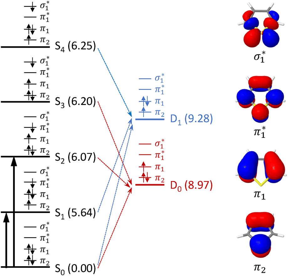

Fig. 2 Left: Electronic configurations of the five lowest singlet electronic states of thiophene and two lowest doublet electronic states of the corresponding radical cation. Numbers in brackets refer to CASPT2(10,9)/6-31G* calculated vertical excited energies and EPT/6-311++G(3df,3pd) vertical ionisation energies, in eV and relative to S₀. Vertical arrows highlight transitions from S₀ to S₁ and S₂. Dashed arrows highlight most probable ionisation processes based on Koopmans' correlations. Right: CASPT2(10,9)/6-31G* natural orbitals.

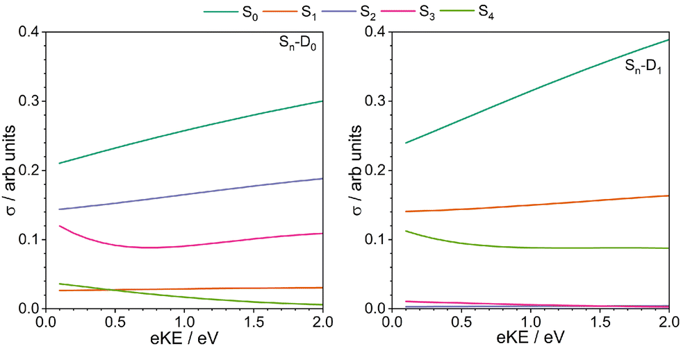Fig. 3 One-photon photoionisation cross-sections from S₀–S₄ to the D₀ (left) and D₁ (right) states of thiophene. Dyson orbital norms were calculated using the EOM-IP-CCSD/6-311++G** method.

3.2. Photoelectron spectra

The 243–234 nm one-colour MPI photoelectron spectra of thiophene are presented as a heat map plotted as a function of eKE and photon energy (Fig. 4). The individual spectra are also plotted as a function of eKE in Fig. 5(a). Fig. 4 allows us to determine whether features in the spectra are a result of non-resonant or resonance-enhanced MPI processes. For non-resonant two-photon ionisation, electrons are emitted with eKE = 2hν − IE, where hν is the photon energy and IE is the ionisation energy. In Fig. 4, the solid black lines highlight peaks in the photoelectron spectra whose eKEs increase at twice the rate of the photon energy, and represent non-resonant ionisation from S₀ to the two doublet cation states, D₀ and D₁. Following resonant photoexcitation of an excited electronic state S_n, with excess vibrational energy E_vib = hν − AEE(S_n) where AEE(S_n) is the adiabatic excitation energy of S_n, ionisation by a second photon will result in the emission of electrons with eKE ≤ 2hν − AIE(D_m) − E_vib = hν − [AIE(D_m) − AEE(S_n)], where AIE(D_m) is the adiabatic ionisation energy of the cation doublet state D_m. In Fig. 4, the dotted and dashed black lines highlight peaks in the photoelectron spectra whose eKEs increase at the same rate as the photon energy, and represent resonance-enhanced ionisation to the two doublet cation states, D₀ and D₁, respectively. The y-intercepts of the solid, dotted and dashed lines were obtained from plots of the MPI photoelectron spectra as functions of two- or one-photon electron binding energy, eBE = nhν − eKE, where n = 2 or 1 (Fig. 5).

Fig. 4 One-colour MPI photoelectron spectra of thiophene plotted as a function of eKE and photon energy. Arrows mark the photon energies employed. The individual spectra were linearly interpolated and normalised to the most intense feature at 0.70 eV eKE, which corresponds to the S₀–D₁ VIE. Direct ionisation to D₀ and D₁ were determined as 8.8 ± 0.1 eV and 9.6 ± 0.1 eV, as shown by the solid lines of gradient = 2. The most probable indirect ionisation processes are marked with dotted and dashed lines with a gradient of 1. These show ionisation via S₂–D₀ and S₁–D₁, respectively (see text).

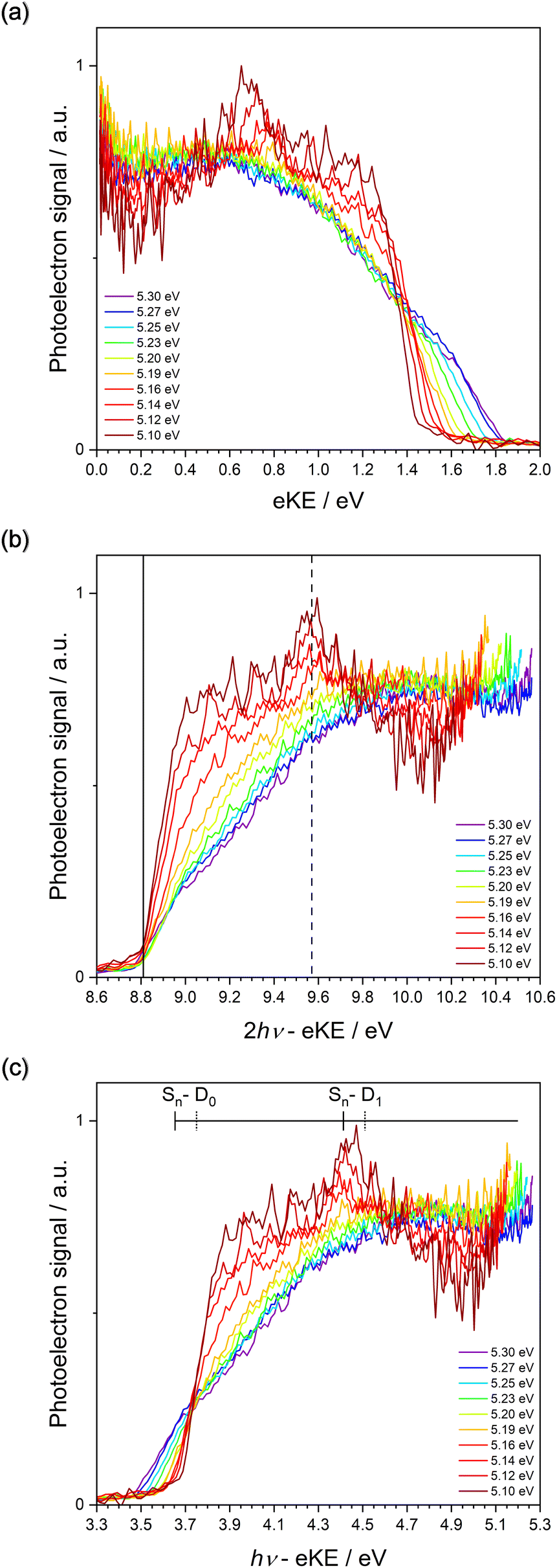Fig. 5 (a) Plot of photoelectron counts versus eKE following 1 + 1 photoionisation of thiophene for 234–243 nm. (b) Plot of photoelectron counts versus two-photon eBE following 1 + 1 photoionisation of thiophene for 234–243 nm. The solid and dashed lines show D₀ = 8.8 ± 0.1 eV and D₁ = 9.6 ± 0.1 eV. (c) Plot of photoelectron counts versus one-photon eBE following 1 + 1 ionisation of thiophene for 234–243 nm. The comb denotes ionisation from S_n–D₀ and S_n–D₁ using the S₁ AEE from Holland et al.,²⁶ the calculated S₂ AEE from Salzman et al.²³ and the ionisation energies from the work reported here. The solid and dashed vertical lines denote adiabatic ionisation from S₁ and S₂, respectively. The individual spectra were normalised to their integrated area.

In Fig. 5(b), the photoelectron spectra are plotted as a function of two-photon binding energy. There are two ionisation energies that can be identified in these spectra. The small bump at 8.8 ± 0.1 eV on the rising edge of the lowest energy peak can be assigned as the S₀–D₀ AIE. This is in excellent agreement with the AIE obtained from PES^{7,9,12,22,36–38,64} and zero-kinetic energy (ZEKE) PES³⁹ measurements, several of which determined that the AIE was equivalent to the VIE (Table 1). The peak at 9.6 ± 0.1 eV is assigned as the S₀–D₁ VIE, and this is also in good agreement with values reported previously.^{7,9,12,22,36–38,64} Note that the errors attributed to our assignments are derived from the uncertainty in the position rather than the energy resolution of our spectrometer.

It can be seen in Fig. 5(b) that the peak attributed to S₀–D₁ does not have any clear vibrational structure (experimental resolution ∼0.05 eV), in agreement with observations of Derrick et al. (experimental resolution ∼ 0.02 eV).³⁷ Also, the peak broadens significantly as photon energy increases, losing the sharpness associated with non-resonant photoionisation from S₀ at photon energies lower that the S₀–S₁ VEE. Although Rydberg states have been observed in the range 9.4–11.8 eV,²⁶ the structured features in our 5.10–5.19 eV photoelectron spectra do not remain at constant eKE with increasing photon energy (Fig. 5(a)) so cannot be attributed to autoionising Rydberg states. Also, the 5.20–5.30 eV photoelectron spectra do not have the identical profiles expected for an autoionising Rydberg states. This leaves two possible explanations for our experimental observations. First, as the photon energy increases above 5.157 eV, S₁ is excited. From Koopmans' correlations (Fig. 2) and calculation photoionisation cross-sections (Fig. 3), the S₁–D₁ ionisation pathway is expected to dominate over S₁–D₀. There may be a large geometric change between S₁ and D₁, which would result in a broader photoelectron spectrum. Moreover, the D₁ feature shifts to higher binding energies with increasing photon energy, which is a signature of resonance-enhanced ionisation from S₁ beginning to compete with, or dominate, non-resonant ionisation from S₀. Second, D₁ could have a short lifetime. Calculations reported by Trofimov et al. identified strong vibronic coupling between D₁ and D₀ and a conical intersection between them,¹⁶ which would account for a short D₁ lifetime and the broad, vibrationally-unresolved photoelectron spectrum.

In Fig. 5(c), the photoelectron spectra are plotted as a function of one-photon binding energy. The comb marks S_n–D_m AIEs determined using AEEs from Holland et al.,²⁶ and Salzmann et al.,²³ and the D₀ and the D₁ IEs from this work. It is clear that S₁–D₁ is the dominant resonance-enhanced ionisation pathway as the photoelectron counts are highest around the calculated S₁–D₁ VIE (4.4 ± 0.1 eV). Nonetheless, there also appears to be a significant contribution from the S₁–D₀ ionisation channel calculated at 3.7 ± 0.1 eV. For photon energies above the S₀–S₁ AEE (5.157 eV), what looks like an isobestic point begins to appear. It lies at 3.7 ± 0.1 eV, which is very close to the calculated S₂–D₀ AIE (3.8 ± 0.1 eV) and is illustrative of an increasing contribution from the population of, and subsequent ionisation from, S₂. Based on Koopmans' correlations and photoionisation calculations, the S₂–D₀ ionisation channel is expected to dominate over S₂–D₁ ionisation, although it is difficult to determine whether there is any significant contribution from S₂–D₁ ionisation from our spectra as they are very congested in the region where we would expect this channel to appear (4.5 ± 0.1 eV). Fig. 3 shows that the cross-sections for the dominant S₂–D₀ and S₁–D₁ ionisation channels are very similar. Population of, and ionisation from, S₂ is consistent with calculations performed by Köppel et al. which reported a rapid population of S₂ following photoexcitation of S₁. At photon energies close to the S₀–S₂ VEE (5.64 eV),³⁴ it is likely that the S₂–D₀ and S₂–D₁ channels would make a larger contribution to the measured photoelectron intensity due to the direct population of S₂.

3.3. Photoelectron angular distributions

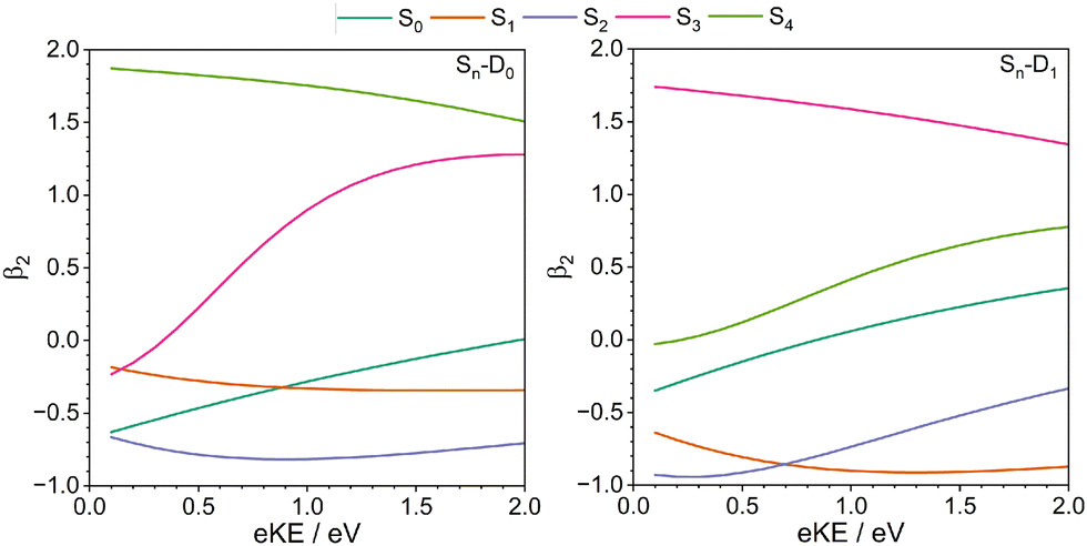
In Fig. 6(a) the measured anisotropy parameter β₂ is plotted as a function of eKE and photon energy. At higher eKEs, between the solid lines marking the upper limits of direct and indirect photoionisation to D₀ and D₁, there is weak anisotropy with β₂ ≈ −0.05. At lower eKEs, below the lines marking the upper limits of direct and indirect photoionisation to the D₁ continuum, the anisotropy changes sign and becomes weakly positive, with β₂ ≈ +0.05. In Fig. 6(b) the measured β₄ anisotropy parameter, is plotted as a function of photon energy and eKE. At higher eKEs, β₄ < 0, whereas for eKE < 0.4, β₄ ≈ +0.1.

Fig. 6 Plots of (a) β₂ and (b) β₄ parameters as a function of eKE and photon energy following 1 + 1 photoionisation of thiophene. The plots have been smoothed using a five-point average for eKE and β parameters. Arrows mark the photon energies employed. The solid lines with gradient = 2 mark the high eKE limits of direct photoionisation to D₀ and D₁. The dotted and dashed lines mark the high eKE limits of indirect S₂–D₀ and S₁–D₁ photoionisation processes, respectively. The grey shaded region is energetically inaccessible via two-photon ionisation.

The calculated one-photon β₂ parameters are plotted in Fig. 7. In the energy region of interest for our experiments, β₂ < 0 for one-photon photoionisation from S₀, S₁ and S₂, to D₀ and D₁. The measured β₂ parameter is a superposition of direct and indirect ionisation processes and although it is negative for higher eKEs, it is positive for lower eKEs. This difference between the calculated and measured patterns could be due to the β₂ parameter for two-photon non-resonant ionisation from S₀ having the opposite sign to our calculated one-photon β₂ parameters for lower eKEs, or it could be the result of structural changes occurring on the timescale of our measurements. Interestingly, β₂ > 0 for photoionisation from S₃ and S₄. Ionisation from S₀–S₂ involve removing electrons from ππ* molecular orbitals whereas ionisation from S₃ and S₄ involve removing electrons from πσ* molecular orbitals. (Fig. 2) This difference in orbital character could explain the difference in sign of the β₂. Thus, another explanation could be that the higher lying S₃ and S₄ states are accessed on the timescale of the measurement, which would be consistent with ultrafast ring-opening. This is indeed found to be the case in our recent theoretical study of the photo-excited dynamics in the vibronically coupled S₁–S₄ states of thiophene.⁶⁵

Fig. 7 Plots of β₂ anisotropy parameters as a function of eKE following one-photon photoionisation from S₀–S₄ to D₀ (left) and D₁ (right) continua, calculated using the EOM-IP-CCSD/6-311++G** method.

Thus, time-resolved photoelectron angular imaging experiments, with supporting calculations of the PADs, could prove valuable for investigating the electronic relaxation pathways following photoexcitation.

4. Conclusions

We have presented 243–234 nm multiphoton photoelectron imaging measurements of thiophene. Plots of the photoelecton spectra as a function of two-photon binding energy allowed us to identify spectral features with binding energies of 8.8 ± 0.1 eV and 9.6 ± 0.1 eV, corresponding to the S₀–D₀ AIE and S₀–D₁ VIE, respectively. These are in excellent agreement with ionisation energies determined using other methods.^{7,9,12,22,36–38,64} Plots of the photoelectron spectra as a function of one-photon binding energy revealed peaks around the S₁–D₁ VIE (4.4 ± 0.1 eV) and S₂–D₀ AIE (3.8 ± 0.1 eV). For spectra recorded with photon energies above the S₀–S₁ AEE (5.157 eV), an isobestic point was observed at hν-eKE = 3.7 ± 0.1 eV illustrating an increasing contribution from S₂–D₀ ionisation, compared with S₁–D₁ ionisation, with increasing photon energy.

Plots of β₂ and β₄ anisotropy parameters as a function of eKE and photon energy suggest that time-resolved photoelectron imaging measurements could provide a sensitive probe of electronic relaxation following UV photoexcitation of thiophene. This work serves as a benchmark for future time-resolved studies of thiophene and more complex molecular systems containing thiophene as a building block that are ubiquitous in many photonic materials.

Author contributions

The project was conceived and supervised by H. H. F. The experimental data were recorded by J. J. B., with technical assistance from M. A. P., and processed, analysed and interpreted by J. J. B. Calculations were undertaken J. J. B., and by S. P. and M. A. P. under the guidance of G. A. W. The manuscript was written by J. J. B. and H. H. F., with contributions from S. P. and G. A. W. All authors read and approved the final version of the manuscript.

Data availability

Data in this article will be made available in the UCL Research Data Repository at https://www.ucl.ac.uk/library/open-science-researchsupport/research-data-management/ucl-research-data-repository.

Conflicts of interest

There are no conflicts to declare.

Acknowledgements

The work was supported by EPSRC grants EP/V026690/1 and EP/L015862/1. The experiments were performed using the Ultrafast Laser Facility in the Department of Chemistry at UCL (EPSRC EP/T019182/1), with technical support from Dr Julia Davies. The authors thank Roisin Tapley for carrying out preliminary calculations of one-photon photoionisation cross-sections and β₂ anisotropy calculations.

Notes and references

1. F. Zhang, D. Wu, Y. Xu and X. Feng, J. Mater. Chem., 2011, 21, 17590–17600.
2. P. Kumaresan, S. Vegiraju, Y. Ezhumalai, S. L. Yau, C. Kim, W. H. Lee and M. C. Chen, Polymers, 2014, 6, 2645–2669.
3. T. Taniguchi, K. Fukui, R. Asahi, Y. Urabe, A. Ikemoto, J. Nakamoto, Y. Inada, T. Yamao and S. Hotta, Synth. Met., 2017, 227, 156–162.
4. G. Kirsch, D. Prim, F. Leising and G. Mignani, J. Heterocycl. Chem., 1994, 31, 1005–1009.
5. H. L. Andriampanarivo, M. Köhler, J. L. Gejo, T. Betzwieser, B. C. Poon, P. L. Yue, S. D. Ravelomanantsoa and A. M. Braun, Photochem. Photobiol. Sci., 2015, 14, 1013–1024.
6. G. Horváth and A. I. Kiss, Spectrochim. Acta, Part A, 1967, 23, 921–924.
7. A. D. Baker, D. Betteridge, N. R. Kemp and R. E. Kirby, Anal. Chem., 1971, 43, 375–381.
8. G. D. Lonardo, G. Galloni, A. Trombetti and C. Zauli, J. Chem. Soc., Faraday Trans., 1972, 68, 2009–2016.
9. P. A. Clark, R. Gleitter and E. Heilbronner, Tetrahedron, 1973, 29, 3085–3089.
10. W. M. Flicker, O. A. Mosher and A. Kuppermann, Chem. Phys. Lett., 1976, 38, 489–492.
11. G. Varsanyi, L. Nyulaszi, T. Veszpremi and T. Narisawa, J. Chem. Soc. Perkin Trans., 1982, 761–765.
12. B. L. Klasinc, A. Sabljic, G. Kluge, J. Rieger, K. Marx Universitat Leipzig, S. Chemie and G. D. Republic, J. Chem. Soc., Perkin Trans. 2, 1982, 539–543.
13. E. J. Beiting, K. J. Zeringue and R. E. Stickel, Spectrochim. Acta, Part A, 1985, 41, 1413–1418.
14. L. Nyulászi and T. Veszprémi, J. Mol. Struct., 1986, 140, 253–259.
15. F. Negri and M. Z. Zgierski, J. Chem. Phys., 1994, 100, 2571–2587.
16. A. B. Trofimov, H. Köppel and J. Schirmer, J. Chem. Phys., 1998, 109, 1025–1040.
17. M. H. Palmer, I. C. Walker and M. F. Guest, Chem. Phys., 1999, 241, 275–296.
18. F. Qi, O. Sorkhabi, A. H. Rizvi, A. G. Suits, C. Sciences, V. Di, E. Orlando and L. Berkeley, J. Phys. Chem. A, 1999, 103, 8351–8358.
19. J. Wan, M. Hada, M. Ehara and H. Nakatsuji, J. Chem. Phys., 2001, 114, 842–850.
20. E. E. Rennie, D. M. Holland, D. A. Shaw, C. A. Johnson and J. E. Parker, Chem. Phys., 2004, 306, 295–308.
21. H. Köppel, E. V. Gromov and A. B. Trofimov, Chem. Phys., 2004, 304, 35–49.
22. R. Weinkauf, L. Lehr, E. W. Schlag, S. Salzmann and C. M. Marian, Phys. Chem. Chem. Phys., 2008, 10, 393–404.
23. S. Salzmann, M. Kleinschmidt, J. Tatchen, R. Weinkauf and C. M. Marian, Phys. Chem. Chem. Phys., 2008, 10, 380–392.
24. G. Cui and W. Fang, J. Phys. Chem. A, 2011, 115, 11544–11550.
25. M. Stenrup, Chem. Phys., 2012, 397, 18–25.
26. D. M. Holland, A. B. Trofimov, E. A. Seddon, E. V. Gromov, T. Korona, N. de Oliveira, L. E. Archer, D. Joyeux and L. Nahon, Phys. Chem. Chem. Phys., 2014, 16, 21629–21644.
27. D. Fazzi, M. Barbatti and W. Thiel, Phys. Chem. Chem. Phys., 2015, 17, 7787–7799.
28. A. Prlj, B. F. Curchod and C. Corminboeuf, Phys. Chem. Chem. Phys., 2015, 17, 14719–14730.
29. A. Prlj, B. F. Curchod, A. Fabrizio, L. Floryan and C. Corminboeuf, J. Phys. Chem. Lett., 2015, 6, 13–21.
30. P. Kölle, T. Schnappinger and R. D. Vivie-Riedle, Phys. Chem. Chem. Phys., 2016, 18, 7903–7915.
31. T. Schnappinger, P. Kölle, M. Marazzi, A. Monari, L. González and R. D. Vivie-Riedle, Phys. Chem. Chem. Phys., 2017, 19, 25662–25670.
32. O. Schalk, M. A. Larsen, A. B. Skov, M. B. Liisberg, T. Geng, T. I. Sølling and R. D. Thomas, J. Phys. Chem. A, 2018, 122, 8809–8818.
33. D. B. Jones, M. Mendes, P. Limão-Vieira, F. Ferreira da Silva, N. C. Jones, S. V. Hoffmann and M. J. Brunger, J. Chem. Phys., 2019, 150, 064303.
34. R. Hakansson, B. Nordén and E. W. Thulstrup, Chem. Phys. Lett., 1977, 50, 306–308.
35. K. L. Reid, Annu. Rev. Phys. Chem., 2003, 54, 397–424.
36. J. H. Eland, Int. J. Mass Spectrom. Ion Phys., 1969, 2, 471–484.
37. P. Derrick, L. Åsbrink, O. Edqvist, B.-O. Jonsson and E. Lindholm, Int. J. Mass Spectrom. Ion Phys., 1971, 6, 177–190.
38. N. Kishimoto, H. Yamakado and K. Ohno, J. Phys. Chem., 1996, 100, 8204–8211.
39. J. Yang, J. Li and Y. Mo, J. Chem. Phys., 2006, 125, 174313–174317.
40. D. Irimia, D. Dobrikov, R. Kortekaas, H. Voet, D. A. Van Den Ende, W. A. Groen and M. H. Janssen, Rev. Sci. Instrum., 2009, 80, 1–6.
41. D. Irimia, R. Kortekaas and M. H. Janssen, Phys. Chem. Chem. Phys., 2009, 11, 3958–3966.
42. G. A. Worth, R. E. Carley and H. H. Fielding, Chem. Phys., 2007, 338, 220–227.
43. D. S. Parker, R. S. Minns, T. J. Penfold, G. A. Worth and H. H. Fielding, Chem. Phys. Lett., 2009, 469, 43–47.
44. A. D. Nunn, R. S. Minns, R. Spesyvtsev, M. J. Bearpark, M. A. Robb and H. H. Fielding, Phys. Chem. Chem. Phys., 2010, 12, 15751–15759.
45. R. S. Minns, D. S. Parker, T. J. Penfold, G. A. Worth and H. H. Fielding, Phys. Chem. Chem. Phys., 2010, 12, 15607–15615.
46. R. Spesyvtsev, O. M. Kirkby, M. Vacher and H. H. Fielding, Phys. Chem. Chem. Phys., 2012, 14, 9942–9947.
47. R. Spesyvtsev, O. M. Kirkby and H. H. Fielding, Faraday Discuss., 2012, 157, 165–179.
48. O. M. Kirkby, M. Sala, G. Balerdi, R. De Nalda, L. Bañares, S. Guérin and H. H. Fielding, Phys. Chem. Chem. Phys., 2015, 17, 16270–16276.
49. S. P. Neville, O. M. Kirkby, N. Kaltsoyannis, G. A. Worth and H. H. Fielding, Nat. Commun., 2016, 7, 11357.
50. O. M. Kirkby, M. A. Parkes, S. P. Neville, G. A. Worth and H. H. Fielding, Chem. Phys. Lett., 2017, 683, 179–185.
51. J. W. Riley, B. Wang, J. L. Woodhouse, M. Assmann, G. A. Worth and H. H. Fielding, J. Phys. Chem. Lett., 2018, 9, 678–682.
52. G. A. Garcia, L. Nahon and I. Powis, Rev. Sci. Instrum., 2004, 75, 4989–4996.
53. S. J. Bajic, R. N. Compton, X. Tang and P. Lambropoulos, Phys. Rev. A, 1991, 44, 2102–2112.
54. P. Celani and H.-J. Werner, J. Chem. Phys., 2000, 112, 5546–5557.
55. M. Richter, P. Marquetand, J. González-Vázquez, I. Sola and L. González, J. Chem. Theory Comput., 2011, 7, 1253–1258.
56. H.-J. Werner, P. J. Knowles, G. Knizia, F. R. Manby and M. Schütz, WIREs Comput. Mol. Sci., 2012, 2, 242–253.
57. H.-J. Werner, P. J. Knowles, P. Celani, W. Györffy, A. Hesselmann, D. Kats, G. Knizia, A. Köhn, T. Korona, D. Kreplin, R. Lindh, Q. Ma, F. R. Manby, A. Mitrushenkov, G. Rauhut, M. Schütz, K. R. Shamasundar, T. B. Adler, R. D. Amos, S. J. Bennie, A. Bernhardsson, A. Berning, J. A. Black, P. J. Bygrave, R. Cimiraglia, D. L. Cooper, D. Coughtrie, M. J. O. Deegan, A. J. Dobbyn, K. Doll, M. Dornbach, F. Eckert, S. Erfort, E. Goll, C. Hampel, G. Hetzer, J. G. Hill, M. Hodges, T. Hrenar, G. Jansen, C. Köppl, C. Kollmar, S. J. R. Lee, Y. Liu, A. W. Lloyd, R. A. Mata, A. J. May, B. Mussard, S. J. McNicholas, W. Meyer, T. F. Miller III, M. E. Mura, A. Nicklass, D. P. O'Neill, P. Palmieri, D. Peng, K. A. Peterson, K. Pflüger, R. Pitzer, I. Polyak, M. Reiher, J. O. Richardson, J. B. Robinson, B. Schröder, M. Schwilk, T. Shiozaki, M. Sibaev, H. Stoll, A. J. Stone, R. Tarroni, T. Thorsteinsson, J. Toulouse, M. Wang, M. Welborn and B. Ziegler, MOLPRO, 2022.1, a package of ab initio programs, 2022, see https://www.molpro.net/.
58. E. Epifanovsky, A. T. B. Gilbert, X. Feng, J. Lee, Y. Mao, N. Mardirossian, P. Pokhilko, A. F. White, M. P. Coons, A. L. Dempwolff, Z. Gan, D. Hait, P. R. Horn, L. D. Jacobson, I. Kaliman, J. Kussmann, A. W. Lange, K. U. Lao, D. S. Levine, J. Liu, S. C. McKenzie, A. F. Morrison, K. D. Nanda, F. Plasser, D. R. Rehn, M. L. Vidal, Z.-Q. You, Y. Zhu, B. Alam, B. J. Albrecht, A. Aldossary, E. Alguire, J. H. Andersen, V. Athavale, D. Barton, K. Begam, A. Behn, N. Bellonzi, Y. A. Bernard, E. J. Berquist, H. G. A. Burton, A. Carreras, K. Carter-Fenk, R. Chakraborty, A. D. Chien, K. D. Closser, V. Cofer-Shabica, S. Dasgupta, M. de Wergifosse, J. Deng, M. Diedenhofen, H. Do, S. Ehlert, P.-T. Fang, S. Fatehi, Q. Feng, T. Friedhoff, J. Gayvert, Q. Ge, G. Gidofalvi, M. Goldey, J. Gomes, C. E. González-Espinoza, S. Gulania, A. O. Gunina, M. W. D. Hanson-Heine, P. H. P. Harbach, A. Hauser, M. F. Herbst, M. Hernández Vera, M. Hodecker, Z. C. Holden, S. Houck, X. Huang, K. Hui, B. C. Huynh, M. Ivanov, A. Jász, H. Ji, H. Jiang, B. Kaduk, S. Kähler, K. Khistyaev, J. Kim, G. Kis, P. Klunzinger, Z. Koczor-Benda, J. H. Koh, D. Kosenkov, L. Koulias, T. Kowalczyk, C. M. Krauter, K. Kue, A. Kunitsa, T. Kus, I. Ladjánszki, A. Landau, K. V. Lawler, D. Lefrancois, S. Lehtola, R. R. Li, Y.-P. Li, J. Liang, M. Liebenthal, H.-H. Lin, Y.-S. Lin, F. Liu, K.-Y. Liu, M. Loipersberger, A. Luenser, A. Manjanath, P. Manohar, E. Mansoor, S. F. Manzer, S.-P. Mao, A. V. Marenich, T. Markovich, S. Mason, S. A. Maurer, P. F. McLaughlin, M. F. S. J. Menger, J.-M. Mewes, S. A. Mewes, P. Morgante, J. W. Mullinax, K. J. Oosterbaan, G. Paran, A. C. Paul, S. K. Paul, F. Pavo, Z. Pei, S. Prager, E. I. Proynov, A. Rák, E. Ramos-Cordoba, B. Rana, A. E. Rask, A. Rettig, R. M. Richard, F. Rob, E. Rossomme, T. Scheele, M. Scheurer, M. Schneider, N. Sergueev, S. M. Sharada, W. Skomorowski, D. W. Small, C. J. Stein, Y.-C. Su, E. J. Sundstrom, Z. Tao, J. Thirman, G. J. Tornai, T. Tsuchimochi, N. M. Tubman, S. P. Veccham, O. Vydrov, J. Wenzel, J. Witte, A. Yamada, K. Yao, S. Yeganeh, S. R. Yost, A. Zech, I. Y. Zhang, X. Zhang, Y. Zhang, D. Zuev, A. Aspuru-Guzik, A. T. Bell, N. A. Besley, K. B. Bravaya, B. R. Brooks, D. Casanova, J.-D. Chai, S. Coriani, C. J. Cramer, G. Cserey, A. E. DePrince, R. A. DiStasio, A. Dreuw, B. D. Dunietz, T. R. Furlani, W. A. Goddard, S. Hammes-Schiffer, T. Head-Gordon, W. J. Hehre, C.-P. Hsu, T.-C. Jagau, Y. Jung, A. Klamt, J. Kong, D. S. Lambrecht, W. Liang, N. J. Mayhall, C. W. McCurdy, J. B. Neaton, C. Ochsenfeld, J. A. Parkhill, R. Peverati, V. A. Rassolov, Y. Shao, L. V. Slipchenko, T. Stauch, R. P. Steele, J. E. Subotnik, A. J. W. Thom, A. Tkatchenko, D. G. Truhlar, T. Van Voorhis, T. A. Wesolowski, K. B. Whaley, H. L. Woodcock, P. M. Zimmerman, S. Faraji, P. M. W. Gill, M. Head-Gordon, J. M. Herbert and A. I. Krylov, J. Chem. Phys., 2021, 155, 084801.
59. J. V. Ortiz, Wiley Interdiscip. Rev.: Comput. Mol. Sci., 2013, 3, 123–142.
60. H. H. Corzo and J. V. Ortiz, Adv. Quantum Chem., 2017, 74, 267–298.
61. J. V. Ortiz, J. Chem. Phys., 2020, 153, 1–28.
62. M. J. Frisch, G. W. Trucks, H. B. Schlegel, G. E. Scuseria, M. A. Robb, J. R. Cheeseman, G. Scalmani, V. Barone, B. Mennucci, G. A. Petersson, H. Nakatsuji, M. Caricato, X. Li, H. P. Hratchian, A. F. Izmaylov, J. Bloino, G. Zheng, J. L. Sonnenberg, M. Hada, M. Ehara, K. Toyota, R. Fukuda, J. Hasegawa, M. Ishida, T. Nakajima, Y. Honda, O. Kitao, H. Nakai, T. Vreven, J. A. MontgomeryJr, J. E. Peralta, F. Ogliaro, M. Bearpark, J. J. Heyd, E. Brothers, K. N. Kudin, V. N. Staroverov, R. Kobayashi, J. Normand, K. Raghavachari, A. Rendell, J. C. Burant, S. S. Iyengar, J. Tomasi, M. Cossi, N. Rega, J. M. Millam, M. Klene, J. E. Knox, J. B. Cross, V. Bakken, C. Adamo, J. Jaramillo, R. Gomperts, R. E. Stratmann, O. Yazyev, A. J. Austin, R. Cammi, C. Pomelli, J. W. Ochterski, R. L. Martin, K. Morokuma, V. G. Zakrzewski, G. A. Voth, P. Salvador, J. J. Dannenberg, S. Dapprich, A. D. Daniels, Ö. Farkas, J. B. Foresman, J. V. Ortiz, J. Cioslowski and D. J. Fox, Gaussian09 Revision E.01.
63. S. Gozem and A. I. Krylov, WIREs Comput. Mol. Sci., 2022, 12, e1546.
64. J. W. Rabalais, L. O. Werme, T. Bergmark, L. Karlsson and K. Siegbahn, Int. J. Mass Spectrom. Ion Phys., 1972, 9, 185–196.
65. M. A. Parkes and G. A. Worth, J. Chem. Phys., 2024, 161, 114305.

---

Footnote

† Electronic supplementary information (ESI) available. See DOI: https://doi.org/10.1039/d4cp02504k

---