
 Open Access Article
 This Open Access Article is licensed under a
 Creative Commons Attribution 3.0 Unported Licence
Non-adiabatic molecular dynamics simulations provide new insights into the exciton transfer in the Fenna–Matthews–Olson complex†
Monja
Sokolov
a,
David S.
Hoffmann
 a,
Philipp M.
Dohmen
ab,
Mila
Krämer
a,
Sebastian
Höfener
a,
Ulrich
Kleinekathöfer
c and
Marcus
Elstner
*a
a,
Philipp M.
Dohmen
ab,
Mila
Krämer
a,
Sebastian
Höfener
a,
Ulrich
Kleinekathöfer
c and
Marcus
Elstner
*a
aInstitute of Physical Chemistry (IPC), Karlsruhe Institute of Technology, Kaiserstrasse 12, 76131 Karlsruhe, Germany. E-mail: marcus.elstner@kit.edu
bInstitute of Nanotechnology (INT), Karlsruhe Institute of Technology, Kaiserstrasse 12, 76131 Karlsruhe, Germany
cSchool of Science, Constructor University, Campus Ring 1, 28759 Bremen, Germany
First published on 9th July 2024
Abstract
A trajectory surface hopping approach, which uses machine learning to speed up the most time-consuming steps, has been adopted to investigate the exciton transfer in light-harvesting systems. The present neural networks achieve high accuracy in predicting both Coulomb couplings and excitation energies. The latter are predicted taking into account the environment of the pigments. Direct simulation of exciton dynamics through light-harvesting complexes on significant time scales is usually challenging due to the coupled motion of nuclear and electronic degrees of freedom in these rather large systems containing several relatively large pigments. In the present approach, however, we are able to evaluate a statistically significant number of non-adiabatic molecular dynamics trajectories with respect to exciton delocalization and exciton paths. The formalism is applied to the Fenna–Matthews–Olson complex of green sulfur bacteria, which transfers energy from the light-harvesting chlorosome to the reaction center with astonishing efficiency. The system has been studied experimentally and theoretically for decades. In total, we were able to simulate non-adiabatically more than 30 ns, sampling also the relevant space of parameters within their uncertainty. Our simulations show that the driving force supplied by the energy landscape resulting from electrostatic tuning is sufficient to funnel the energy towards site 3, from where it can be transferred to the reaction center. However, the high efficiency of transfer within a picosecond timescale can be attributed to the rather unusual properties of the BChl a molecules, resulting in very low inner and outer-sphere reorganization energies, not matched by any other organic molecule, e.g., used in organic electronics. A comparison with electron and exciton transfer in organic materials is particularly illuminating, suggesting a mechanism to explain the comparably high transfer efficiency.
1 Introduction
Light-harvesting complexes (LHCs) in photosynthetic organisms are responsible for the harvesting of solar light and the subsequent transfer of energy to the reaction center. They are typically found in aggregates or supercomplexes,1 where a unit of an LHC consists of a protein scaffold embedding several pigment molecules. The energy transfer efficiencies of LHCs can be extremely high, which has sparked interest in the detailed mechanisms. The Fenna–Matthews–Olson (FMO) complex of green sulfur bacteria is one of the most studied LHC complexes, on the one hand because its crystal structure was already solved in the 1970s2 and on the other hand because of its relatively small size, which made it a suitable toy model for theoretical approaches. Furthermore, the complex gained particular interest after the detection of long-lived quantum beats,3,4 which finally led to a discussion about the role of quantum coherence5,6 and possibly even entanglement7–9 in the energy transfer process.The FMO complex is located between the chlorosome, a large organelle containing thousands of different pigment molecules that harvest sunlight, and the cytoplasmic membrane containing the reaction center (Fig. 1a). The FMO complex is a homotrimer and each monomer contains seven bacteriochlorophyll a (BChl a) pigments. An additional eighth BChl a pigment is more loosely attached to each monomer (Fig. 1b). This pigment probably represents the entrance of energy from the chlorosome, since it is expected to interact with the paracrystalline baseplate10 on the side of the chlorosome closest to the cytoplasmic membrane.11 The connection between an FMO trimer and a reaction center was recently revealed in detail by cryo-electron microscopy.12 Surprisingly, the C3 symmetry axis of the FMO trimer was found at an angle of 75% against the reaction center and not perpendicular to it. The authors of ref. 12 suggest that this arrangement supports the energy transfer to the reaction center via the BChl 3 of two FMO monomers. As a consequence, only two of the three BChl 8 pigments receive energy from the chlorosome.
 | ||
| Fig. 1 (a) Location of the FMO complexes in the photosynthetic apparatus of green sulfur bacteria.12 (b) From left to right: a trimer with the seven pigments in orange and the eighth pigment in red, arrangement of the BChl a pigments in one monomer with their numbering, and chemical structure of BChl a. | ||
In general, energy transfer in LHCs occurs via excitons, which can be localized to single pigments or distributed over several pigments. The amount of delocalization is determined by the relative excitation energies of the pigments (site energies) and the couplings between the pigments. The site energies are tuned by the protein environment mainly through electrostatic interactions and geometrical distortions. The couplings in contrast are mainly tuned by the pigments' distances and orientations, which are determined by the protein scaffold. The temperature-dependent vibrations of the pigments and their environment cause fluctuations in the site energies and couplings. Furthermore, the relaxation of the pigment geometry after excitation and the reaction of the environment to the new electronic state play a role in the energy transfer process by lowering the site energies by the amount of the reorganization energy.
The FMO complex has been studied experimentally using a variety of spectroscopic techniques, and many experiments are performed at cryogenic temperatures. However, a temperature effect on the energy transfer is expected due to an increased dynamical disorder. Green sulfur bacteria have been found in hot springs,13 so the transfer must be robust at ambient and higher temperatures. Of special interest is to understand the efficiency of the exciton transfer. The exciton transfer in FMO occurs in the sub-picosecond to picosecond regime with high quantum yields and therefore ultrafast, as reported in many experimental studies to date.14–22 It occurs on a similar time scale to that of ultrafast photochemical events such as light-induced isomerization of chromophores like retinal, and therefore much faster than many charge or energy transfer events in proteins, which occur on a micro-second to second timescale. This is surprising, since the distance traveled is quite large, but the driving force of a few tenths of millielectronvolt and the excitonic couplings are quite small, as many theoretical studies have shown.11,23–33 Nevertheless, the sub-picosecond dynamics has been confirmed by simulations based on density matrix or ensemble averaged wave-packet dynamics, finding a fast decay of the exciton to site 3 in most cases. As Maity and Kleinekathöfer28 wrote, ‘… the exciton leaves the initially excited pigment in a roughly exponential manner and is first transferred to BChl 2 and subsequently to the rest of the network.’ The obvious question, therefore, is what is the source of this efficiency and the transmission mechanism.
The oscillations observed in 2D spectra4,18,20–22,34 initially led to the suggestion that quantum mechanical effects may play a vital role in this efficiency. Today, it is no longer assumed that the oscillation results from electronic coherences, as summarized by Cao et al.35 Instead, nuclear vibrations have been suggested to couple to the electronic systems, thereby fostering the efficient transfer. Runeson et al.36 investigated several models concluding that a pure classical picture can explain the energy funnel, but the discussion is far from being closed.22,37
So far, many dynamical simulations have been based on simplified models of the electronic structure using a Frenkel Hamiltonian.28,38,39 They often feature a high-level description of the quantum dynamics, while the coupling to the protein environment is described by time-independent pre-determined or estimated spectral densities. In some cases also ensemble-averaged wave packet dynamics, e.g., in the form of the numerical integration of the Schrödinger equation (NISE), have been performed on pre-computed trajectories, i.e., without back-reaction of the system dynamics on the environment25 though some attempts have been tested in which this back-reaction has been included.40 One focus of these studies was to investigate the role of electronic and/or nuclear quantum effects in the efficiency of the exciton transfer. For the description of photochemical events a seemingly orthogonal strategy has been established in the last few decades: here, the emphasis lies on an accurate representation of the electronic structure of the chromophores and the electrostatic coupling of the chromophores to the protein environment, while nuclei are treated classically in most implementations. For this purpose, semi-empirical density functional theory (DFT) or ab initio methods are used to compute energy and forces ‘on the fly’ following electronically excited states. Since state crossing can occur, non-adiabatic molecular dynamics (NAMD) techniques are applied, the most prominent being Tully's surface hopping (TSH) approach.41,42 In general, NAMD simulations allow the propagation of nuclear and electronic degrees of freedom simultaneously, i.e., the PES of the electrons is computed ‘on the fly’, and no pre-computed parameters have to be used. The coupling to the protein environment is achieved using embedding methods like QM/MM techniques.43–45 The energy landscape of the FMO chromophores and the different exciton couplings are an outcome of such a formalism and are computed ‘on the fly’, rather being a model input. The advantage of these methods is the possibility to sample molecular fluctuations explicitly,46 and although nuclear quantum effects can be included in principle, most implementations are based on classical nuclear trajectories. While these methods have been mostly used for single chromophores, the application to extended and multi-chromophoric systems comes with new challenges.47 The simulations of LH by the Martinez group using a highly efficient QM implementation provided detailed information, which can be gained using such an approach, but the study itself was limited to a single very short trajectory.48 To compute observables such as transition times, a large number of longer trajectories must be evaluated, which is currently not possible with standard NAMD approaches, since for the simulation of long time scales for these large systems, the standard methodology cannot be applied in a straightforward manner.49
Despite the considerable amount of theoretical studies on FMO, obtaining information on the exciton transfer mechanism and the reasons for its efficiency remains a challenge because it requires ‘a holistic approach that considers structure, energetics, dynamics, disorder, and fluctuations all together’.1 As mentioned by several authors,1,37 ‘on the fly’ quantum chemical excited state trajectory calculations would be highly desirable. In practice, however, such simulations, which need to run for tens of picoseconds, are still far too expensive.1 In order to reach the required time-scales for large, multi-chromophoric systems like FMO or LH2, we combined several computational strategies into a complex multi-scale method with the following features: (i) the electronic structure is fragmented, leading to a Frenkel-Hamiltonian representation of the electronic structure, which is computed ‘on the fly’ along NAMD simulations. (ii) Since even semi-empirical quantum chemistry methods like DFTB or MNDO-derivatives would be too expensive, specifically trained neural networks are used to represent the electronic structure. (iii) The coupled electronic–nuclear degrees of freedom are then propagated using TSH. This leads to a linear scaling of computing time with the system size and allows for extensive sampling in the picosecond time scale.
The advantage of such a method is that it represents a bottom-up approach with well-tested simplifications to compute the relevant electronic parameters, which – due to fragmentation – have a physical meaning and can be tested independently. The method is based on a Frenkel Hamiltonian, i.e., it uses parameters well known in this field, which we have extensively benchmarked in a previous work.33 A further approximation allows the use of a pre-computed reorganization energy λ, which is a critical parameter for the dynamical simulations and which will be critically assessed in this work. The neural networks (NNs) are then trained to compute these parameters ‘on the fly’ along the dynamic simulations. We have applied such a scheme to fast electron transfer in photolyases and chryptochromes50–55 and to electron transfer in organic semiconductors.56–62 This fragmentation method is also able to simulate exciton transfer in organic materials63,64 and will be applied to exciton transfer in biosystems in this work for the first time. Since the same methodology has been extensively tested for electron and exciton transfer in organic semiconductors, for which experimental data for mobilities and diffusion lengths are available, the good agreement found in these studies lends confidence to the results in this work. This is in line with previous findings that a fragmentation into a Frenkel exciton model can satisfactorily reproduce the full ab initio results.65
We will carefully compare the parameters relevant in this work with high-level calculations and references from the literature and test our results regarding their sensitivity to a meaningful range of values. Because of the efficiency of our approach, we are able to run multiple sets of propagation simulations under different conditions, each set consisting of a statistically meaningful number of simulations. Moreover, we were able to follow the actual path of a single exciton, which was not possible with Ehrenfest-based approaches that only provide a mean-field picture.
As Mukamel66 pointed out one can distinguish two types of coherences: the first is exciton delocalization and the second is coherence resulting from a superposition of eigenstates due to excitation with a laser pulse. While the second type has been ruled out to be the reason for FMO exciton transfer efficiency,35 delocalization67,68 has been discussed to be a critical factor for understanding the efficiency of charge60,61,69,70 and exciton transfer64,71 in organic materials. The charge and exciton transfer efficiency (mobility and diffusion) is strongly correlated with delocalization. The simulations reported in this work indicate that a similar mechanism to that found in organic materials seems to be at work also in FMO, i.e., exciton transfer can be understood on the basis of classical nuclear dynamics, where the electronic system fulfills special conditions to feature exciton delocalization. In particular, the very low reorganization energy of the BChl a pigments, compared to those of molecules studied in organic materials, seems to be at the core of the surprising efficiency.
This article is structured as follows: first, we describe the key ingredients of our method, discuss the critical parameters for a successful simulation, and demonstrate the performance of the NNs applied to speed up the calculations. In the Results section, we analyze our exciton propagation simulations and discuss the sensitivity of the choice of parameters. A comparison with charge and exciton transfer in organic materials allows understanding the mechanism and efficiency of the exciton transport in FMO and potentially other light-harvesting systems.
2 Methods
In recent years we have developed a methodology that allows the treatment of fast electron and exciton transfer processes and have applied this methodology to a variety of problems ranging from electron transfer in DNA and photolyases50,53,54,72–76 to electron and exciton transfer in organic materials.56–63 Since this transfer involves a large number of atoms, ranging from hundreds to thousands, very large quantum regions must be handled. Furthermore, the coupling of the quantum region to the environment is crucial.In this study, we simulate the exciton motion through the FMO complex in a mixed quantum-classical approach, applying a combination of strategies as in our previous works. In short, the method is based on (i) an embedding approach using coupled quantum mechanical molecular mechanics (QM/MM) methods, (ii) a fragmentation approach applied in the QM region and (iii) non-adiabatic molecular dynamics (NAMD), where the relevant electronic degrees of freedom are propagated with the electronic Schrödinger equation coupled to the nuclear degrees of freedom that are treated classically. The basic methodology has been introduced in ref. 63, where it was applied to anthracene, and has been extended using a machine learning Hamiltonian in ref. 59. For charge transfer we have substituted the kernel ridge regression method by NNs recently62 because of the large training sets required. NNs are also the method of choice in this work. The extension to biological chromophore systems such as FMO and LH2 makes extensive use of the developments introduced to study charge transfer processes, which we will describe in detail in the following. Due to the high methodological similarity, benchmarking for organic materials has proven to be very helpful, since experimental data on the transport mechanism and the charge mobility or exciton diffusion length are available, which could demonstrate the reliability of the methodology.56–58,60,61,63
2.1 Quantum mechanics/molecular mechanics scheme
In QM/MM simulations we partition the system into the quantum mechanical (QM) region, where the exciton is situated and is governed by the principles of quantum mechanics, and the molecular mechanical (MM) region, which represents the environment and is governed by a classical force field. We use a so-called subtractive QM/MM scheme,77 where the MM force field covers the whole system including the quantum region leading to the total energy for excitons as| Etot = EMM + ΔEexQM + ΔEQM/MM. | (1) |
Consider now an excitation to a particular excited state, e.g., the S1 state, then ΔEexQM represents the S0–S1 excitation energy. One could now run Born–Oppenheimer Molecular Dynamics (BOMD) simulations on that state and forces can be readly derived by taking the derivatives of Etot (eqn (1)) with respect to nuclear coordinates of every term as:
| Ftot = FMM + ΔFexQM + ΔFQM/MM. | (2) |
2.2 The Frenkel Hamiltonian
The excitation can extend over several molecules and travel within the QM region. In order to generate an efficient representation of ΔEexQM we use three further approximations: (i) we represent the excitation using a Frenkel Hamiltonian, (ii) compute its matrix elements using the cost efficient semi-empirical TD-LC-DFTB2 method and (iii) in order to allow for extended dynamical simulations we train NNs to predict the matrix elements on the fly even more efficiently.First, we divide the QM zone into several fragments, which can be computed separately. This leads to the Frenkel Hamiltonian (eqn (3)) consisting of the excitation energies εn of individual chromophores and excitonic couplings Vnm, which are computed for pairs of monomers using the Coulomb approximation (Coulomb coupling). The Frenkel Hamiltonian thus describes the supermolecular excitations using molecular excitations as basis states. Hence, we consider only locally excited states and neglect the contributions from charge transfer states, which will be included in future work.
 | (3) |
Despite the (relative) efficiency of the TD-LC-DFTB2 method, the computational cost for direct application to multi-chromophoric systems such as FMO and LH2 is still high, since we have to sample extensively to obtain convergent results for the non-adiabatic MD simulations. Basing the method on the Frenkel-Hamiltonian makes the problem linear-scaling with the molecule number, requiring only a few individual QM/MM excited state calculations for the whole complex per time step (7 calculations for one FMO monomer). Nonetheless, the evaluation of the site energies and couplings remains the bottleneck. To further speed up the method, we apply machine learning (ML) techniques and learn the Frenkel-Hamiltonian elements based on a data set derived from TD-LC-DFTB2 calculations, as described in more detail below.
2.3 Coupled equations of motion for nuclear and electronic degrees of freedom
The complete system is divided into two parts: the nuclear degrees of freedom, which are described by standard empirical force fields, and the electronic degrees of freedom. The dynamics of the electronic part is described by the solution of the time-dependent Schrödinger equation, where the Hamiltonian is given by eqn (3). To propagate both nuclear and electronic degrees of freedom simultaneously, we employ a NAMD scheme.In a first step, we expand the general exciton state
 | (4) |
 | (5) |
For the solution of the electronic Schrödinger equation, besides Ehrenfest several propagation methods are available. We have thoroughly evaluated several approaches for the systems of interest, i.e., the propagation of excitons (or electrons) through multi-chromophoric systems, in ref. 60. The Trajectory Surface Hopping (TSH) method82 proved to be the most suitable and allowed the prediction of experimental mobilities with very good accuracy,61 which shows that the representation of both the electronic structure of the problem and the electronic dynamics is achieved quite satisfactorily. The coupling between the electronic and nuclear degrees of freedom of the pigments is described by the surface hopping propagator with the fewest switches.
Neither Ehrenfest nor TSH pre-determine a charge or exciton transfer mechanism, but predict hopping or coherent transfer depending on the details of the system of interest. Being approximate, the propagation methods have different strengths and shortcomings. In contrast to mean-field trajectory methods such as the Ehrenfest method, TSH propagates the nuclei on a single adiabatic potential energy surface (PES), and there is a certain probability for a hop from one PES to another when the surfaces approach each other or cross. It is important in this context that both the chromophore structure and electrostatic environment respond to the presence of the exciton, leading to what is known as inner and outer-sphere reorganization energies. In contrast, in an Ehrenfest scheme the wave function will evolve into a superposition of both states, which poses a problem for representing both the inner and outer sphere reorganization energies. Since the quantum state is given by a superposition of two (or more) adiabatic states, the molecule deforms and the environment polarizes according to this superposition, which leads to the well known mean-field problem of Ehrenfest dynamics. As a result, reorganization energy will not be accounted for properly, and in some cases it may be completely missed out, as we demonstrated for charge transport in DNA in some detail.51,52 Furthermore, TSH can estimate the delocalization of the exciton, since the wave-function only refers to single excitons and not to an ensemble as in Ehrenfest, which quickly spreads out in the system.
Being an approximate propagation scheme, TSH has several drawbacks, i.e., it has no rigorous derivation from first principles, it prevents the system from transforming into a superposition of adiabatic states through the hopping algorithm and usually the quantum nature of nuclei is not taken into account. Non-classical effects, as discussed in the introduction, are therefore neglected in this work. Furthermore, many trajectories have to be computed in order to allow for appropriate averaging.
To apply Tully's fewest switches surface hopping (FSSH) method, we have to represent the equations of motion in terms of adiabatic states.60,63 Diagonalization of the Frenkel Hamiltonian (eqn (3)) for any nuclear conformation of the molecules in the QM region leads to the Hamiltonian Had and the adiabatic eigenstates |ψi〉 of the system with eigenenergies Ei. The energies and wave-function coefficients bin are computed from
| Had = UHFrenkelU†, | (6) |
 | ||
| Fig. 2 Scheme of the propagation algorithm used in this work. Explanations are given in the text. Please note that the adiabatic energies Ei are actually the differences between the adiabatic excited state energies and the ground state energies and are denoted ΔEi in the text. | ||
The solution of the time-dependent Schrödinger equation preserves wavefunction coherence. To account for the coupling to the complex environments, most TSH implementations to date apply a decoherence correction. Furthermore, the application to multi-chromophoric systems like organic materials or FMO faces the so-called trivial crossing problem, for which also a correction scheme has been developed. We adopt these two corrections as described in ref. 60 and 63 as well.
In TSH, the electronic degrees of freedom are propagated using eqn (5), coupled to the propagation of the nuclei according to Newton's equation of motion. For this we have to evaluate the forces according to eqn (2). FMM results from the force field. In the FSSH method, the nuclei are propagated on a single electronic state i, the active surface. Therefore, ΔFexQM from eqn (2) is the difference in excited state and ground state forces:
| ΔFexQM = FexQM − F0QM | (7) |
 where ΔEi denotes the difference between the adiabatic energy of the current state ‘i’ and the QM ground state energy. This formulation is used because it will allow the use of a Δ machine learning approach in future work in order to account for this term explicitly. In this work, we use an approximate scheme, which has the advantage to describe the effect of excited state relaxation by a single parameter, as described in the next section, the reorganization energy. This allows a systematic testing of different reorganization energies, as discussed in the Results section.
The third force contribution in eqn (2) results from the derivative of the QM/MM interaction term ΔEQM/MM in eqn (1). This effect is covered within an atomic point charge model by the QM/MM term (eqn 8). Please note that this term is dependent on the exciton occupation |bin|2 in the active state i, i.e., additional forces are only in place for the occupied sites.
 | (8) |
2.4 Approximations for an efficient surface hopping algorithm
The straightforward application of FSSH involves the calculation of ground and excited state forces according to eqn (2), which is followed by computing hopping probabilities.60,63 To assure energy conservation after a hop, i.e., after a change in the active surface, typically, the change in the potential energy is compensated by a scaling of the velocities in the direction of the non-adiabatic coupling vector (NACV). Both the calculation of excited state forces and NACVs is tedious and can be avoided by using further approximations introduced and tested recently for electron transfer.(i) The computation of the NACV elements can be substituted by using the Boltzmann-corrected fewest switches surface hopping variant (BC-FSSH) as described and tested in detail in ref. 60 and 61. The velocities of the pigment atoms after a hop are not adjusted as usual but the hopping probability itself is corrected by a Boltzmann factor to preserve the total energy averaged over an ensemble of trajectories. This eliminates the need to determine the NACVs and does not cause significant loss of accuracy for the systems tested so far.
(ii) An explicit treatment of excited states and their forces can be substituted by two approximations. If an exciton hops from one site to the other, two main changes occur: the geometry relaxes and the charge density changes. These two changes manifest themselves in two well known effects, the inner and outer sphere reorganization energies.
The first effect is the lowering of the site energy by the inner sphere reorganization energy, as discussed in detail in our earlier work.50–52 This effect can be effectively treated by a modification of the diagonal elements of the Hamiltonian as61
| εn → εn − λ|an|2. | (9) |
 and implicitly treating the effective energy decrease by modifying the Hamiltonian according to eqn (9). Since the reorganization energy, i.e., the response of the chromophores to excitation, has been shown to be very sensitive to the quantum chemical method applied,83,84 this approach has the big advantage of being able to treat reorganization energies as accurately as possible. For some systems, only high level methods can account for this effect with sufficient accuracy. Since reorganization energy occurs in Marcus theory in the exponential, while excitonic (electronic) couplings only appear as prefactors, an appropriate treatment of λ seems to be even more sensitive than high accuracy in the coupling calculations. Our extensive tests on charge transfer in organic materials have shown that both approximations, IR and BC, only lead to a slight increase in mobilities compared to the exact procedure (ref. 61) of calculating forces with a particular DFT functional. However, it has the advantage of choosing the parameters computed with a level of theory, which has the required accuracy.
The second effect is given by the outer sphere reorganization energy, i.e., the response of the protein environment to the change in charge density due to excitation, which is covered by the QM/MM interaction term as discussed above.
A scheme of the propagation code summarizing all relevant steps is shown in Fig. 2. At the beginning of the simulation, the exciton is placed on one or more pigments of choice by assigning the initial values of the wavefunction coefficients in the input file. The current conformation of the system provides the inputs for the NNs. The NNs predict the elements of the Frenkel Hamiltonian. Subsequently, the correction for the relaxation of the populated pigments is made in this transfer Hamiltonian. Diagonalization of the Frenkel Hamiltonian corresponds to a transformation from the diabatic picture into the adiabatic picture. The transformation matrix U is used to convert the diabatic coefficients into the adiabatic coefficients and vice versa. The total wavefunction of the exciton can be expressed as a linear combination of the diabatic basis functions with coefficients an (eqn (4)). The exciton is propagated by integrating the time-dependent Schrödinger equation (TDSE) with a smaller time step, using the transfer Hamiltonian. As a result we obtain new coefficients of the total wavefunction. Then a hop is attempted using these new coefficients in the adiabatic basis. A probability for the hop is computed and subsequently compared to a pseudo-random number. If a hop occurs, a decoherence correction is first applied and the active surface i changes. If not, the active surface remains the same, but still the pigment occupations (|bin|2) changed. Therefore, in both cases, the force field charges of the pigments are adjusted according to the new pigment occupations. With the new force field charges, all nuclei in the system are propagated with Newton's equation of motion (EOM) and the input for the NNs for the next cycle is provided.
2.5 Hopping vs. delocalized transfer
Using Marcus theory, localized transfer can be described using three parameters, the driving force ΔG ≈ Δε between the sites, the couplings V (= Hmn) and reorganization energy λ. Fragment orbital (FO)-based NAMD simulation techniques are able to describe the transition between localized and delocalized transport.60,61,64 Organic semiconductor materials with high mobilities brought up the question about the appropriateness of transfer of localized charges/excitons, i.e., the straightforward application of Marcus hopping type models. One can find two types of arguments, which are also relevant in the context of FMO exciton transfer:(i) Troisi85 emphasized a possible ‘speed limit’ for charge transfer to be described by hopping models, which is based on time scale separation: the use of a parameter for reorganization energy requires the molecular relaxation to be on a much faster time scale than the hopping events, i.e., that relaxation happens instantaneously compared to hopping. For organic molecules, this is no more the case if mobilities are larger than 0.1 cm2 V−1 s−1. The relevant time scale is given by the C–C stretching vibrations, i.e., the molecule cannot adapt to the new electronic state faster than within a period of this vibration. As the analysis of the exciton dynamics below shows, we find several hops within 100 fs, i.e., at the time scale of this vibration. A second factor is the relaxation of the protein environment, leading to outer-sphere reorganization energy, which definitely happens on a longer time scale, discussed in quite some detail by Matyushov86 for biological electron transfer. We have found such a situation in the fast charge transfer in photolyases and chryptochromes,50,53,54,72–76 where the fragment based NAMD formalism proved to be very useful. Straightforward application of a simple Marcus hopping approach underestimates the rates by orders of magnitude, and a frequency dependent calculation of λ86 could be a viable correction also for these systems.
(ii) A second, related limit for the validity of Marcus theory is the relation between couplings and reorganization energy. Exciton or charge transfer is an activated process only for small couplings compared to reorganization energy. For an isoenergetic two-state model this relation can be quantified by a simple formula.64,87 For |V| ≪ λ/2 the transport mechanism is given by Marcus hopping, for |V| ≫ λ/2 the barrier vanishes and the localized hopping picture breaks down. Although hopping rates can still be formally computed, they are meaningless. Sometimes accidental agreement with experiment is found, however, due to wrong reasons as discussed in ref. 60. Although in FMO the site energies are not isoenergetic and this relation cannot be derived in the same way, the site energies are close enough in energy that a similar threshold can be expected. The reason for high mobilities in organic semiconductors has been related to this breakdown of hopping, leading to a transport model termed transient localization theory (TLT). This model bridges the transport regime between band and hopping models and features an efficient transport due to delocalization over few molecules. This feature can also be shown in direct simulations of the type applied in this work.56,60,61,64,70 As discussed below, the transport parameters in the FMO approach |V| ≈ λ/2, and therefore, a similar transport picture is expected.
3 Computational details and accuracy
3.1 System and MD simulations
The studied system consists of one solvated FMO monomer from Chlorobaculum tepidum with the seven Bacteriochlorophyll a (BChl a) pigments embedded in the protein scaffold. The CHARMM27 force field was used for the protein, the TIP3P model for the water molecules and BChl parameters from ref. 88 and references therein. We performed MD simulations at 300 K and 77 K, using Gromacs version 2021.5.89–91 In all production runs at 300 K, the temperature was maintained by the Nosé–Hoover thermostat92,93 using a time step of 1 fs and the pressure of 1.013 bar was controlled by the Parrinello–Rahman barostat.94,95 Periodic boundary conditions and the Particle Mesh Ewald method for long-range electrostatics were used. We created two different production runs at 300 K using slightly different conditions. This was done not only to increase the number of starting structures for our propagation runs, which contributes to better statistics, but also to enable a rough estimation of the degree of dependence of our findings on simulation conditions. The two runs are denoted as set 1 and set 2 in the following.set 1: The details of the equilibration procedure have been reported before.33,96 The simulation was run for 20 ns to sample the relevant conformations of the pigment–protein complex with a time step of 1 fs and no constraints were applied. The structures sampled in this MD simulation at 300 K were used to generate the training data for our machine learning models.
set 2: We performed a second independent MD simulation at 300 K under slightly different conditions as follows: the crystal structure (pdb-ID: 3ENI) was prepared using standard Gromacs tools.89 Missing residues were modeled using the MODELLER web service97 and the complex was solvated in a cubic water box with a side length of 9.427 nm (contains more water than the box from set 1). One Cl− ion was added to neutralize the system. We first minimized the system using the steepest descent algorithm until all forces were below 1000.0 kJ mol−1 nm−1 and then used the conjugate gradient algorithm to further reduce the maximum force to a value below 100.0 kJ mol−1 nm−1. Equilibration was performed in three steps. First, velocities were generated and an NVT ensemble was simulated for 1 ns using the Nosé–Hoover thermostat to maintain the temperature at 300 K. Bonds involving hydrogen were constrained and the positions of the heavy atoms of the protein and the BChl chromophores were restrained with a force constant of 1000 kJ mol−1 nm−1. The time step was set to 1 fs. As a second step, we simulated an NPT ensemble for 1 ns with a reference pressure of 1.013 bar using the Parrinello–Rahman barostat. The time step, constraints and restraints were the same as in the previous step. The position constraints were finally removed for the next equilibration step, which was another 1 ns NPT simulation under otherwise the same conditions. The system was then simulated for 20 ns, but the first 10 ns were discarded as additional equilibration time. Periodic boundary conditions and the Particle Mesh Ewald method for long-range electrostatics were used in all steps.
At 77 K we performed in total six independent simulations: the first five simulations result from the 300 K MD simulations by cooling down five equally spaced snapshots from the first 10 ns of set 1. Cooling down was achieved by performing a 2 ns NVT equilibration with a 1 fs time step and a Nosé–Hoover thermostat. Then a 25 ns NPT equilibration was performed with a 1 fs integration step, Nosé–Hoover thermostat and Parrinello–Rahman barostat to maintain the target pressure of 1.013 bar. Finally, a productive simulation was performed for 100 ns with a 2 fs time step and hydrogen bond constraints using the LINCS algorithm. The Nosé–Hoover thermostat and the Parrinello–Rahman barostat were used. These five simulations will be referred to as set 3 through set 7. For the sixth simulation we heated up the energy minimized crystal structure to 77 K using the same protocol for NVT and NPT. Since the density had not yet converged, two further NPT simulations, first for 20 ns and then for 100 ns, were performed before starting the productive run. This simulation will be referred to as set 8. No restraints on heavy atoms were required for any of the productive or equilibration runs due to the slow movement of the atoms.
The ground state MD simulations were used to generate training or test data for the NNs or to create starting structures for NAMD propagation simulations.
3.2 NAMD simulations
The propagation of the electronic and nuclear degrees of freedom as described in Section 2.3 is based on Gromacs version 4.6, coupled with our in-house charge/exciton transfer code. A small integration time step of 0.1 fs was used in the MD steps of the NAMD simulations. For every combination of parameters or conditions evaluated in this paper, we ran 100 NAMD simulations with a length of 10 ps each, see Table 1. The 100 different initial structures at 300 K were taken from the MD simulations at 300 K, either from set 1 or set 2. The structures of both of these sets stem from 10 ns of the corresponding MD simulation (the first 10 ns in the case of set 1) and are evenly spaced by 100 ps. The 100 different initial structures of the NAMD simulations at 77 K accordingly stem from one of the MD simulations at 77 K, which are denoted sets 3–8. In this case, the structures are evenly distributed over the complete 100 ns and are hence spaced by 1 ns.| Simulation | Description |
|---|---|
| set 1 | 20 ns, 300 K |
| set 2 | 10 ns, 300 K, diff. conditions |
| set 3 | 100 ns, 77 K, start from set 1, frame 0.0 ns |
| set 4 | 100 ns, 77 K, start from set 1, frame 2.5 ns |
| set 5 | 100 ns, 77 K, start from set 1, frame 5.0 ns |
| set 6 | 100 ns, 77 K, start from set 1, frame 7.5 ns |
| set 7 | 100 ns, 77 K, start from set 1, frame 10 ns |
| set 8 | 100 ns, 77 K, start from pdb 3ENI |
The simulations were initiated with the exciton assigned to one pigment, which was either pigment 1 or pigment 6 as will be indicated in the text below. This is a common practice in the literature, e.g. ref. 34, 98 and 99, since these pigments are most likely the entrances of the energy coming from the baseplate/pigment 8. This may be seen as a reasonable starting point, since the ‘true’ adiabatic states are very difficult to localize: (1) due to the fast fluctuations of the site energies, the adiabatic states in the system change not only their diabatic populations, but also their energetic order very often. Both facts lead to a drastic change in the diabatic populations of one single adiabatic state that was defined as the nth state with respect to energy. As an example, we show the time-dependent populations of the first adiabatic state for a trajectory in Fig. S48 in the ESI.† The states fluctuate strongly at 300 K and change their character within a few tenths of femtoseconds. Therefore, there is an uncertainty due to the duration of the laser pulse whether really only a certain adiabatic state is excited. (2) With respect to the photoexcitable states, we refer to the uncertainty principle that leads to a broadening in the range of tens of meV for femtosecond laser pulses. As an example, we have shown the eigenvalues of the first and second adiabatic states in Fig. S49 in the ESI,† which differ on average by 26 meV. Therefore, at high temperatures no single adiabatic state may be excited, anyways.
3.3 Charges
Ground state BChl parameters were taken from ref. 88, and the change in charges Δqα due to excitation as occuring in the QM/MM interaction term in eqn (2) was computed as follows: partial charges for BChl a (without the phytyl tail) in both the ground state and the first excited state were determined from a fit to the electrostatic potential obtained from (TD-)DFT at the CAM-B3LYP100/def2-TZVP level using the KOALA program.101 For these calculations a geometry optimized in the ground state with B3LYP102–104/6-31+G(d,p) using Gaussian 09105 was used. The differences between these ground state and excited state charges were added as corrections to the force field charges of the excited pigments. If a pigment was only partially occupied by the exciton, accordingly only a fraction of the difference was added to the charges. The charges are reported in the ESI,† Table S4.3.4 Reorganization energies
The implicit relaxation approach requires knowledge of the inner sphere reorganization energy of the BChl a pigments in FMO. This value is expected to be close to the Stokes shift of BChl a in a vacuum, i.e., the difference between the excitation energies calculated on the ground state geometry and the S1 geometry. For most molecules this property is quite straightforward to compute and ab initio calculations indicate that the DFT functional ωB97X-D is quite accurate for this purpose, while gradient corrected and even hybrid functionals like B3LYP tend to underestimate this property.106 For chlorophylls, surprisingly large errors can occur and the choice of method is not obvious at all. Rätsep et al.83 reported both calculated and experimental reorganization energies in triethylamine, which allows for calibration of methods. The experimental reorganization energies for absorption and emission presented for fivefold coordinated magnesium at 295 K are λabs = 335 cm−1 and λem = 185 cm−1, and so the total reorganization energy is λ ≈ 0.064 eV. Higashi et al.84 addressed this issue in a DFT study of excited states of BChl a and also presented a comparison of theoretical reorganization energies in the gas-phase and in triethylamine. The best agreement with experiment in triethylamine was achieved by CAM-B3LYP with the specially optimized partition parameter μ = 0.20. The gas-phase reorganization energy calculated with this method is λ = 310 cm−1 (≈0.038 eV). Our own calculations with B3LYP/6-31+G(d,p) (neglecting the phytyl tail) gave λ ≈ 0.035 eV, which is close to the best CAM-B3LYP estimate and the previous B3LYP calculations in ref. 83 and 84.The outer sphere reorganization energy is treated in our MD simulations through eqn (2) explicitly, i.e., the excitation introduces a different charge model, which leads to a response of the complex environment. Rivera et al.31 computed outer sphere reorganization energies of 15–20 cm−1 (≈2 meV), which appear to be quite low compared to the inner sphere reorganization energy. The experimental value for triethylamine solvent, which has a dielectric constant (εr = 2.4) similar to that of a protein environment, is much larger. To study the effect of reorganization energy systematically, we used besides our calculated value of 0.035 eV also the much larger experimental estimate 0.065 eV from ref. 83. These two values should represent upper and lower bounds of the inner sphere reorganization energy.
3.5 Coupling corrections
Exciton couplings, which are used for the NN training, are computed from TD-LC-DFTB2 and have been shown to agree well with references using DFT and ab initio methods.33,79–81 There are, however, suggestions in the literature claiming that for accurate calculations of spectral properties some corrections should be applied. We therefore have investigated two of these corrections and modified the LC-DFTB2 couplings accordingly.The first correction refers to the applied charge model used to compute the Coulomb couplings. The transition dipole moments calculated from these charges (≈7.5 D on average) are overestimated compared to the experimental value (≈6.1 D23,107). Such an error in the charge model has also been observed for TD-DFT/B3LYP, which was previously used to determine transition charges for TrESP couplings.25,108 Usually the charges are simply scaled to the experimental value.23,25 For TD-LC-DFTB2, this results in a factor of 0.656 (≙ factor 0.81 for the transition charges) to correct for the overestimated TD-LC-DFTB2 vacuum couplings.
While this first scaling factor corrects the charge model, a second factor is typically applied to account for the polarizability of the medium between two pigments. Scholes et al.109 found an empirical formula to determine a reasonable scaling factor as a function of the distances between different pigments in different photosynthetic proteins. We have calculated this scaling factor using the distances between the centers of mass of the BChl a pigments without phytyl tails. It is roughly between 0.56 and 0.68, but of course it differs for different pigment pairs and snapshots.
In this work, we therefore compare three coupling models, the TD-LC-DFTB2 couplings, the scaled ones (the first scaling factor applied) and the scaled and screened ones (the first and second scaling factors applied). These three values should represent reasonable upper and lower bounds of the couplings.
3.6 LC-DFTB accuracy
Since LC-DFTB is used to train NNs, we briefly discuss site energies and couplings computed from this model in comparison to previous results. Since all chromophores are identical, differences in site energies result from different geometries, the interaction with the protein environment and differences in solvent exposure. Therefore, the exact energy spacing is dependent on the specific QM/MM model used, i.e., the QM and the MM methods applied, and the structural model on which the calculations are based on.Differences in values can hence arise from several sources: (i) as we have shown in detail for the retinal chromophore, different quantum chemical methods compute a different environmental response.33,110 For instance, LC-DFTB2 and also B3LYP underestimate the environmental response using an electrostatic QM/MM embedding method, i.e., the energy spacing may be slightly underestimated. (ii) Furthermore, different charge models in the various force fields may also have a small contribution to these differences, e.g., ref. 111, and (iii) protein polarization effects may reduce the energy spacing compared to QM/MM approaches with a point charge model. Therefore, the underestimation using LC-DFTB2 or B3LYP in combination with neglecting polarization may show a compensating effect.
Furthermore, crystal structures may exhibit a different electrostatic interaction compared to MD averages, and further, as shown before,112 site energies may change on very long time scales. We find therefore a sizable effect of the MD conditions on the energy spacing, as shown by our results for set 1 and set 2 (see Section 3.1).
There are a large number of articles presenting calculated site energies in FMO (species C. tepidum and P. aestuarii), e.g., ref. 25–27, 29, 32, 113, and 114, or site energies from a fit of optical spectra, e.g., ref. 23, 115–119 and there are also several review articles, e.g., ref. 1, 24, and 120. All computational methods differ as specified above; the computed effects are small compared to the accuracy of the methods, and therefore differences should not be overinterpreted. The energy differences are mostly within kBT, and the differences between the various approaches are surprisingly minute, having in mind the accuracy to be expected from QM/MM methods. We present our site energies in comparison to some selected examples in Fig. 3 and refer to the literature otherwise. A benchmark of TD-LC-DFTB2 BChl site energies is already given in ref. 33 and 121.
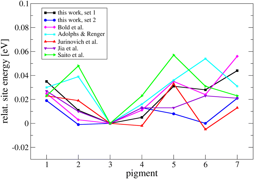 | ||
| Fig. 3 Site energies of the pigments obtained from Gaussian fits to TD-LC-DFTB2 results compared to literature values. All site energies in this plot have been shifted so that the corresponding energy of pigment 3 is zero. Bold et al.33,121 determined TD-LC-DFTB2 site energies in a previous study. Adolphs and Renger23 determined site energies from fits to optical spectra. Jia et al.27 used ZINDO/S, and Jurinovich et al.26 and Saito et al.29 used TD-DFT. Configurations were taken from MD simulations. However, the force fields, treatment of the environment, FMO species, etc. are different. | ||
A similar picture arises regarding excitonic coupling calculations. We compared our couplings with literature values in the ESI† (Fig. S2 and S3) and computed the (averaged) adiabatic energy spectrum and absorption spectra (Fig. S10–S14, ESI†). As a result, we think that the scaled (by a factor of 0.656) but not screened couplings give the best agreement with the existing body of research, and therefore we use these couplings as the default ones in the simulations. However, we also perform simulations with the other two couplings (unscaled, scaled and screened) to estimate the effect of small variations in these couplings on the dynamics of the system.
3.7 Machine learning
NNs were used to predict the elements of the transfer Hamiltonian, i.e., the site energies and the couplings. Two different networks were trained, one for the site energies and one for the couplings. The training data for both networks were obtained from a classical MD simulation (set 1, see above).For the site energies, a common model was trained for all seven BChl a pigments, so that a total of 140![[thin space (1/6-em)]](https://www.rsc.org/images/entities/char_2009.gif) 000 structures were obtained from 20000 snapshots of the trajectory with an equal spacing of 1 ps. The site energies were calculated with the semi-empirical TD-LC-DFTB2 method using a parameter set optimized for excitation energies.79–81 The phytyl tail of the BChl a pigments was neglected to reduce the number of atoms per pigment from 140 to 85. It is known that the site energies of the BChl a pigments in the FMO complex are tuned by the protein environment, see e.g. ref. 26 and 121. The range between the lowest and highest site energies increases when the specific pigment environment is included in the calculation. For this reason, we considered the electrostatic potential (ESP) induced on the pigment atoms in our TD-LC-DFTB2 calculations using an in-house variant of the DFTB+ program. The electrostatic potential at the location of a QM atom α of pigment n
000 structures were obtained from 20000 snapshots of the trajectory with an equal spacing of 1 ps. The site energies were calculated with the semi-empirical TD-LC-DFTB2 method using a parameter set optimized for excitation energies.79–81 The phytyl tail of the BChl a pigments was neglected to reduce the number of atoms per pigment from 140 to 85. It is known that the site energies of the BChl a pigments in the FMO complex are tuned by the protein environment, see e.g. ref. 26 and 121. The range between the lowest and highest site energies increases when the specific pigment environment is included in the calculation. For this reason, we considered the electrostatic potential (ESP) induced on the pigment atoms in our TD-LC-DFTB2 calculations using an in-house variant of the DFTB+ program. The electrostatic potential at the location of a QM atom α of pigment n was calculated within the nearest image convention along the simulation trajectory according to eqn (10). It corresponds to the sum of the NMM charges QA of the MM atoms read from the force field divided by their distances rαnA to the pigment atoms.
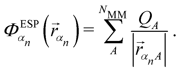 | (10) |
The second network was trained to predict the couplings between the pigments. Only the strongest coupling pairs were considered, namely 1–2, 2–3, 3–4, 4–5, 5–6, 6–7 and 4–7. The other non-nearest neighbor couplings are clearly smaller;25–27,121 see also Table S3 in the ESI.† The reference values were calculated using the same MD trajectory as for the site energies. The phytyl tail was truncated and the transition charges were calculated as an approximation of the transition densities with TD-LC-DFTB2 in a vacuum. The transition charges were used to compute Coulomb couplings. The network architecture for the couplings is similar to the network architecture for the site energies. The only differences are that the distances between each atom of the first pigment and all other atoms of the second pigment are used as input and the ESP is not considered. The input distances allow distinguishing different relative orientations of the pigment pairs, i.e., the NN is set up to learn the signs of the couplings as well. Possible corrections to the couplings (scaling, screening) were done during the propagations after the NN predictions, and so the NN predicts the raw TD-LC-DFTB2 results. The training settings were the same for site energies and couplings. Of the total 140000 reference examples, 20000 were separated for testing. The remaining training set of 120000 was divided into 108000 examples for actual training and 12000 validation examples. The initial learning rate for the Adam optimizer was 1 × 10⁻⁴. Overfitting was prevented by an early termination callback with a patience of 250 epochs. The maximum number of epochs was set to 2000.
000 training examples, R2 values above 0.9 were achieved (see ESI,† Fig. S16). The final R2 scores and mean absolute errors (MAEs) for 120000 training examples are shown in Table 2. The R2 scores improved up to 0.99 and the MAEs are in the meV range.
000 examples). The training set contained 120000 examples
| Site energies | Couplings | |
|---|---|---|
| R 2 score | 0.990 | 0.991 |
| MAE [eV] | 0.004 | 0.001 |
Fig. 4 visualizes the predicted values on the test sets compared to the reference values by means of scatter plots (Fig. 4(a), (b)). To estimate the quality of this prediction, we further analyze the NN performance by showing the predictions against the TD-LC-DFTB2 reference results along a short trajectory segment. Fig. 4c shows the results for the site energies of pigment 1 and Fig. 4d the couplings between pigments 1 and 2. The plots for the other pigments and pigment pairs can be found in the ESI† (Fig. S17 and S18). Obviously, there is almost perfect agreement between the predicted and reference site energies for all pigments. The deviations of the predicted values are very small compared not only to the absolute site energies but also to their fast fluctuations. A particularly well predicted pair of couplings along this trajectory section is 5–6. For some couplings we occasionally see a different trend in their fluctuations, e.g., coupling 2–3. In some cases the amplitude of the fluctuations even differs significantly between the predicted and reference values, e.g., coupling 4–7. Despite these details, we find that the overall trend is mostly correct, but the question remains how much these deviations impact the estimation of observables. In previous work we have performed a more detailed analysis probing also the effect of ML accuracy on charge transfer mobilities. These tests show that the small deviations in the time series do not impact observables like charge mobility.59,62 To test the site energies in our case, we compared the computed spectral densities. Critical deviations should be reflected in the spectral density, since the energy-driven transport pathway is sensitive to fluctuations in site energies driven by the system-bath coupling, what this property exactly resembles.
 | ||
| Fig. 4 Quality of the NNs. (a) and (b) Scatter plots showing the performance of the NNs to predict site energies and couplings of the respective test sets. The colours from blue over pink to yellow indicate the number of points in a certain area. (c) and (d) Performance of the NNs in the last 200 fs of a 10 ps simulation in comparison to the LC-DFTB2 reference values. The values shown are unmodified (no subtraction from the site energies and no scaling of the couplings). (e) Spectral densities obtained from NN predictions and DFTB calculations. | ||
We used a 60 ps QM/MM simulation of each individual chromophore with the DFTB3 method, using the 3OB-f parameters developed for vibrational properties.122 We first compared the distribution of TD-DFTB computed and NN predicted excitation energies for pigment 1 in Fig. S47 (ESI†), finding a very good overlap of the histograms taking into account that the NN has been trained for force field structures. We then computed the spectral density using the TD-DFTB computed and NN predicted site energies, respectively. In a recent work we have shown that 3OB-f parameters allow the computation of spectral densities in very good agreement with experimental results.99Fig. 4e shows that the NN predicted parameters lead to a very good agreement with the TD-DFTB computed results, showing the precision of the NN for this task. Please note that the NN is trained on force field structures since the NAMD simulations are also based on those when using the implicit relaxation (IR) method as introduced above.
For the 77 K simulations, we did not need to retrain the NNs, because the variance of the geometries, energies and couplings at 77 K was very small. Therefore, the NNs trained on 300 K data performed well on 77 K geometries in a cross-validation (see Fig. S19 in the ESI†). This holds also for the other 300 K structures from set 2, as the cross validation in the ESI,† demonstrates (Fig. S20).
Even if we had to retrain the NNs for 77 K and set 2 data, the overall time savings in NAMD simulations would be well worth the extra effort of retraining. The fast semi-empirical reference method TD-LC-DFTB2 takes ≈94 s per calculation of a site energy and ≈57 s for the transition charges in a vacuum (the computation times are averages over 70000 calculations from the training data, respectively, 93% run on Intel(R) Xeon(R) CPU E5-2630 v3@2.40 GHz and 7% on Intel(R) Xeon(R) Silver 4214 CPU@2.20 GHz). However, the trained NNs predict a site energy in only ≈1.4 ms and a coupling in ≈1.6 ms (determined on Intel(R) Xeon(R) CPU E5-2630 v3@2.40 GHz as average over 70000 predictions of the same structures as evaluated for the TD-LC-DFTB timings), resulting in a speed-up factor of about 50000. The average running time of the propagation simulations with the NN and our default conditions was ≈70 min per ps (on Intel(R) Xeon(R) Silver 4214 CPU@2.20 GHz). With an estimated time of more than 100 days instead with TD-LC-DFTB, the use of NNs is not only a preferable option, but acts as a door opener for running NAMD simulations in the ps regime.
There are many approximate ways to compute the exciton couplings. A very fast method is definitely using constant transition charges, which may be accurate enough for many applications and would not need an NN. An indication for this may be the tests we performed with constant couplings, as discussed below. However, we wanted to implement a general scheme, which allows us to access the whole range of coupling calculations, from fixed charge over fluctuating charge or even using supermolecule calculations, which will allow us to test the assumptions in future work also on other LH systems. The NN is extremely fast, so that it makes no significant difference in computation time compared to a coupling calculation with given constant transition charges.
4 Results
In this section, we first analyze exciton dynamics at 300 K using the parameters that we consider to be the most realistic ones. Then we discuss the effects of variation of parameters and temperature.4.1 Mechanism and pathways at 300 K
As discussed above, 100 NAMD simulations were started with structures from set 1 at 300 K, with the exciton initially located at pigment 1. We used the vacuum couplings predicted by our NN scaled by a factor of 0.656. The effect of coupling strength as discussed above on the dynamics is explicitly investigated below. The reorganization energy for implicit relaxation was set to the computed value of 0.035 eV, and outer sphere reorganization energy was explicitly taken into account through the QM/MM interaction.Fig. 5a shows the time development of the site occupations averaged over all 100 trajectories. Site 1 is rapidly depopulated within 500 fs, and a steady state is reached after about 1 ps. This exponential decay of the population to site 2 as an intermediate with final relaxation to a stationary state as shown in our ensemble of trajectories has been described by several density matrix or Ehrenfest like simulations before.28–32 Small differences may arise due to differences in the site energies and/or couplings as a result of different computational approaches and can be regarded as insignificant, since, as discussed above, they are within the accuracy of the quantum chemical methods and structural models used. Fig. 5b shows a normalized histogram of the diabatic occupations summed over all 100 simulations. Pigment 3 is the most occupied one, closely followed by pigments 4 and 2. It is also evident that the exciton is rarely located on pigment 7. These results follow from the site energy distribution discussed above and agree with the picture of ref. 18 based on ref. 23, which assumes that pigment 7 is not significantly involved in any exciton state and that pigments 5 and 6 would belong to the highest lying exciton state.
 | ||
| Fig. 5 (a) Time series of relative populations of the individual BChl a pigments and (b) histogram showing the relative occupations of the individual BChl a pigments, determined from all 100 propagation simulations, respectively. | ||
In a NAMD surface hopping approach this ensemble behavior results from averaging over a sufficient number of trajectories, i.e., our NAMD simulations model an incoherent ensemble by choosing 100 uncoupled starting structures and following 100 uncoupled trajectories, i.e., the description of coherent wave packets is ruled out from the beginning.
In principle, observables are computed for the ensemble, and the use of trajectories has a primarily technical reason: as described above, the focus on single exciton trajectories in TSH allows accounting for the effect of both inner and outer sphere reorganization energies. The dynamics of the exciton through the system leads to a structural response of the chromophores and environment, which in turn impacts the energy landscape of the exciton. In Ehrenfest (mean-field) dynamics this structural response is only given as mean response, grossly underestimating the impact of reorganization energy in cases where it is important.51,52
There is, however, information that can be gained from single trajectories, although they are themselves not observable. First, one gains some insight into the diversity of single exciton dynamics underlying the ensemble behavior. Furthermore, it is possible to compute the delocalizaion of the exciton, a property not accessible in an ensemble approach, since in the latter the wave-function spread refers to the ensemble. From the delocalization, information about the transport mechanism can be derived, since it is related to the transfer barrier and diffusion length as discussed recently.64
Fig. 6 shows how single excitons propagate along the pigments (diabatic occupancy of the seven sites vs. simulation time) for some exemplary simulations. Interestingly, the exciton is mostly transferred from pigment 1 to pigment 2 in much less than a picosecond and also leaves pigment 2 quite rapidly towards sites 3 and 4, i.e., the individual dynamics does not reflect the dynamics of the ensemble, which appears to be an average behavior. Since the site energies fluctuate and the fluctuations are larger than the site energy differences (see ESI,† Fig. S4, S5 and Table S1), the excitons after initial relaxation do not reside on the lowest energy site 3 but undergo a random walk, which allow them to sample all other sites even within the ps-regime, as can be seen in the 2D plots. In other words, since the energy differences are on the order of kBT, we see a thermal diffusion between all sites also on the longer time scale. Therefore, the transfer of the exciton to the reaction center from site 3 is in competition with the random movement of the exciton through the FMO complex, however, with the largest probability to find the exciton on site 3, where it is rather localized.
 | ||
| Fig. 6 The diabatic occupation of the seven pigments is indicated by colors and plotted versus simulation time. Six out of the 100 trajectories are shown (according to their numbering). The exciton is initially localized on pigment 1 and propagates a few times through the whole complex in the 10 ps of simulation. | ||
It is interesting to note that the pigments 1–2–3–4–5–6–7 are connected by sizable exciton couplings, while other connections show small or vanishing couplings, as detailed above. Therefore, the system effectively consists of a quasi-linear chain of chromophores, and the exciton dynamics can only occur along this linear arrangement since all other couplings have been neglected. We investigate this assumption in more detail below. Therefore, starting at site 1, the exciton can relax to sites 2 and 3, and from there it can travel to sites 4 to 7. Only a small coupling connects sites 4 and 7 directly, which also allows for a direct transition between these two sites.
The 2D plots in Fig. 6 further show that the exciton is fairly localized on pigments 1, 2, and 3, but tends to delocalize slightly on pigments 4, 5, 6, and 7. The amount of delocalization can be quantified by the so-called Inverse Participation Ratio (IPR)61
 | (11) |
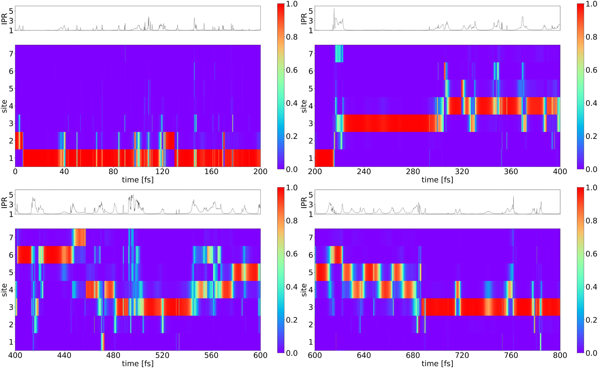 | ||
| Fig. 7 Higher time-resolution of one trajectory (trajectory 40). The diabatic occupation of the seven pigments is indicated by colors and plotted versus simulation time. The IPR vs. time is shown on top of each figure. | ||
While in most trajectories in Fig. 6 the exciton leaves site 1 quite quickly, in trajectory 100 it stays about 100 fs on site 1. This is possible since the total reorganization energy is equal to or higher than the site energy differences, i.e., the exciton can indeed be stabilized at this site. It is the fluctuations of site energies which drive it out of this state. The IPR as shown on the top of the graphs is not constant over time, and the average value of 1.37 results from averaging over long periods of strict localization and short periods, where the exciton is delocalized over two or three sites mostly. When a localized exciton moves between two sites, it must travel via a transition state where it is shortly delocalized between the two sites, and we see many short spikes with an IPR of 2. There a transit happens or is ‘attempted’.
We further see several periods of about 10–30 fs along the trajectory, where the exciton is delocalized over mostly two sites. The longer periods of delocalization, however, indicate, that there may indeed be delocalized exciton states during the relaxation dynamics, as proposed in various experiments.17,18,20 This, however, dominantly happens when the exciton is localized on pigments 4, 5, 6, and 7.
To inspect the occurrence of delocalization, we counted how often the exciton is localized on one or two sites simultaneously by using a certain threshold for the wave function coefficients an. If the coefficients of neighboring sites are both larger than 0.2 (or 0.3) then these two sites are counted as support for a delocalized exciton during that period. Histograms displaying the raw counts are shown in the ESI,† in Fig. S36 and S37. Since some sites are more frequently occupied than others, we normed the counts of the individual pigments with the respective total number of counts involving that pigment. Fig. 8a shows thus the percentage of snapshots in which the individual pigments carry an exciton alone and how often they share a delocalized exciton with another pigment. The result for trajectory 40 (Fig. 8a) indeed confirms that pigments 4 to 7 are more likely delocalized than pigments 1, 2 and 3. If all 100 trajectories are considered, the same trends are observed, but the detailed contributions change slightly (Fig. 8b).
 | ||
| Fig. 8 Percentages of snapshots in which the pigments carry the exciton alone (blue) and in which they share the exciton with another pigment (other colors). The contributions of the different pairs involving the respective pigment are sorted by size (red: largest, pink: lowest). The criterion for a delocalized exciton is an occupation of at least 0.3 on both pigments. | ||
Why are excitons delocalized dominantly on sites 4 to 7 and not on sites 1 to 3? Since all sites are chemically identical, inner sphere reorganization energies cannot account for that behavior. An analysis of outer sphere reorganization energies for substantial differences revealed that more solvent accessible sites tend to have higher reorganization energies, see ref. 31, but this holds only for site 2 but not for sites 1 and 3. A notable difference, however, is seen in the couplings. Average couplings are much larger between sites 4 and 7 than those between 1 and 3. The 4–5, 5–6 and 6–7 couplings are unscaled on average between 15 and 20 meV (scaled: 10–13 meV) and nearly double of the 1–2 and 2–3 couplings (see ESI,† Fig. S2 and Table S2). These values come close to half of the reorganization energies, which – in a Marcus picture – means a barrierless transport and a delocalized exciton as discussed above.87
Inspection of trajectory 40 in the first 500 fs in Fig. 9 indeed shows that the occupation is about 1 for the first three sites in the first 300 fs and delocalization occurs only for short times during transfer between two sites. Once the exciton moved to the sites 4 to 7, it is more delocalized and occupation of 1 is only transiently reached from 500 to 700 fs. Now transfer happens more rapidly, since due to delocalization the reorganization energy is effectively reduced. For the inner-sphere reorganization energy this can be seen from eqn (9); occupations of |an|2 < 1 lead to a smaller reduction of energy, i.e., a smaller stabilization. A similar argument holds for outer sphere reorganization energy, since the charge distribution of a delocalized exciton will have a reduced interaction with the environment, as discussed for electron transfer, where a delocalized hole has a much lower reorganization energy than in the transfer of a spatially confined hole.51,123
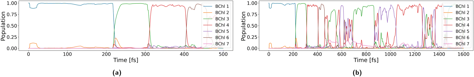 | ||
| Fig. 9 Population of sites along trajectory 40 during the first (a) 500 fs and (b) 1.5 ps. | ||
The funnel to pigments 3 and 4 is expected, since they are the closest to the reaction center. Different pathways of the exciton have been discussed in several previous studies on FMO. For example in ref. 27, a scheme is shown based on calculated site energies and couplings alone (see also ref. 31). This is in qualitative agreement with our findings in that two independent pathways are proposed ending at pigment 3, one from pigments 1 and 2 and the other one from pigment 6 over 5 or 7 and finally 4. Our studies suggest that starting from site 6 a similar picture would arise with a relaxation to sites 3 and 4 followed then by a diffusion to sites 1 and 2.
As mentioned above, an ensemble picture will report a relaxation dynamics towards the most stable sites, while simulations of single exciton transfer events find a thermal diffusion between the accessible states at temperature T. At 300 K, we see a dynamics involving all states, and at 77 K, as described below, this picture changes drastically. Furthermore, fine details of the dynamics may depend on energy differences of within 0.01 eV, which are impossible to describe using current quantum chemical methods. Chemical accuracy, which is defined as an accuracy within 1 kcal mol−1 (= 0.043 eV), is achieved only with very accurate post-Hartree Fock methods, and this accuracy is not reached with current DFT approaches, not to speak of more approximate methods currently used in the FMO field. Therefore, our methods provide a qualitatively correct picture, which may be quantitatively modified in the future. This concerns the values of the site energies and the couplings, which determine the localization/delocalization features discussed.
4.2 Excitation of site 6 at 300 K
Both site 1 and site 6 are close to the base-plate. They can be equally excited, therefore leading to two exciton pathways. Since, however, the localization/delocalization features seem to be different at the two pathways, it is interesting to study the dynamics starting from site 6 as well. Using the same initial structures, we started 100 simulations with an exciton initially localized at site 6. As shown in Fig. 10a the decay starting from site 6 is much faster than the decay starting from site 1, which can be explained by the much larger delocalization of the exciton. | ||
| Fig. 10 Population of sites in propagation runs at 300 K with initial excitation of pigment 6. | ||
The delocalization can be directly seen by inspecting the time-dependent populations for different trajectories. Starting at site 1, the exciton is quite localized during the first 300–400 fs, i.e., in Fig. 9 we see a quite localized hopping picture. Starting the simulations at site 6, we see a rapid delocalization for the three trajectories as displayed in the three lower panels of Fig. 10. Similar information can be extracted from the 2D plots as shown in Fig. S35 in the ESI.† The larger delocalization directly leads to a faster transfer, as discussed above.
At 300 K, we see a random walk of the excitons between the FMO chromophores, with dominant occupancy of site 3. The details of the dynamics and the average occupations may depend on the precise values of the site energy, which is sensitive to the computation method and structural model used, but the overall picture of fast transfer is not affected by these details. In the simulations so far, we did not consider the couplings between sites 1 and 6. As shown in Section 4.4, although small, they may allow a transfer between these sites, which is not covered by the simulations presented so far.
The finding that relaxation from site 6 is faster than that from site 1 has been reported before.34 Using a non-local Master equation approach based on a Frenkel Hamiltonian and a spectral density fitted to experimental data, they reported a significant faster decay from site 6 than that from site 1 at 300 K. While in both cases the relaxation occurs within a picosecond time-scale, starting from site 6 their simulations show a similarly fast decay within 400 fs, as shown in Fig. 10.
4.3 Scaling of the couplings and impact of reorganization energy
In the previous subsection we used a single scaling factor to correct for the overestimation of the TD-LC-DFTB2 transition charges. As discussed in the Methods section, it has been suggested to account for the screening of the couplings by the environment with an additional screening factor.109 Details and a comparison of unmodified, scaled, and both scaled and screened couplings are provided in the ESI.† Whether the screening is necessary or not is debatable and probably within the error bars of the ab initio calculations usually performed. Furthermore, screening may not be necessary because the MMPol couplings from ref. 26 are closer to the scaled but unscreened couplings. However, in order to get an idea of upper and lower bounds of the used parameters, we present the results with the scaled and screened couplings as a limiting case (lower limit).We analyzed simulations with initial structures from set 1 and set 2, as indicated in the tables. The exciton was initially localized on pigment 1. The size of the couplings clearly affects the delocalization of the exciton. Table 3 shows the average IPR obtained with unmodified and with scaled and screened couplings for two different values of the reorganization energy, which also affects the delocalization of the exciton. When a scaling and screening factor is used, the exciton is basically localized on one pigment on average (IPR ≈ 1.2 pigments). If our couplings are not decreased at all, the delocalization is about 1.5 pigments. A lower reorganization energy favors delocalization.
| set 1 | Unmodified couplings | Scaled | Scaled and screened |
|---|---|---|---|
| λ = 35 meV | 1.59 | 1.37 | 1.23 |
| λ = 65 meV | 1.44 | 1.26 | 1.15 |
| set 2 | Unmodified couplings | Scaled | Scaled and screened |
|---|---|---|---|
| λ = 35 meV | 1.60 | 1.38 | 1.22 |
| λ = 65 meV | 1.46 | 1.27 | 1.17 |
Remarkably, we do not reach an average delocalization over two to three pigments as previously assumed.18,23 Even the IPR in the limiting case with unmodified couplings and a reorganization energy of 35 meV is only over approximately 1.6 pigments. But as discussed in the last section, the delocalization is highly fluctuating and a temporary delocalization can easily reach two to three sites, and even more. This finding is quite dependent on the size of the couplings (see ESI,† Fig. S23–S25).
Fig. 11 shows the initial decay of the ensemble populations (i.e., averaged over 100 simulations) for the three different coupling sizes. For λ = 35 meV, the decay behavior seems to be in agreement with the experimental decay, although the unscreened seem to be on the fast side, while the scaled and screened couplings seem to be on the slow side of the expected outcome. Going to λ = 65 meV, the behavior systematically shifts, and the scaled and screened decay seems to be quite slow; however, for the larger couplings the decay also seems to be within a reasonable range. As discussed above, it is the ratio of couplings to reorganization energy that impacts the dynamics, and therefore, the uncertainty of both parameters has to be taken into account. The results show, however, that our investigated parameter space indeed marks reasonable upper and lower limits of both couplings and reorganization energies. The decision on this space is based purely on theoretical considerations, and we see that it agrees with the experimental outcome. Although the effect of the parameters seems to be modest concerning the experimental outcome, it is more dramatic looking at the microscopic events as shown in Fig. 12. The dynamics of the individual exciton depends, on a sub-ps time-scale, quite drastically on the parameters, as indicated by the hopping events shown by the time-dependent occupation. This can also be seen by inspecting the 2D graphs in the ESI† (Fig. S23).
 | ||
| Fig. 11 Averaged diabatic populations of the pigments during the 100 NAMD simulations of set 1 with the exciton initially localized at pigment 1. (a) Unscaled and unscreened couplings with λ = 35 meV, (b) scaled but not screened couplings with λ = 35 meV (default), (c) scaled and screened couplings with λ = 35 meV, (d) unscaled and unscreened couplings with λ = 65 meV, (e) scaled but not screened couplings with λ = 65 meV, and (f) scaled and screened couplings with λ = 65 meV. | ||
 | ||
| Fig. 12 Diabatic populations of the pigments during the NAMD simulation of set 1 with the exciton initially localized at pigment 1. All propagations started with the same starting structure conformation number 40 of set 1. | ||
4.4 Effect of fluctuations
In this section, we investigate the effect of fluctuations of site energies and couplings on the exciton dynamics. For this, we run the dynamics (a) with constant site energies but couplings allowed to fluctuate according to the nuclear dynamics and (b) with constant couplings, where the site energies are allowed to fluctuate. Basically, we just substitute in (a) constant site energies and in (b) constant couplings in the NAMD simulations as described above.Removing the site energy fluctuations (a) has a drastic effect on the exciton propagation. In a first step we use the average values from set 1 (all 20000 snapshots per pigment considered). The initial relaxation of the populations, averaged over 100 trajectories, is shown in Fig. 13a. Although pigment 1 is rapidly depopulated to site 2, no equilibration to the lower energy sites 3 and 4 occurs when the steady state is reached. Example 2D trajectories are shown in the ESI† (Fig. S26). After initial fast relaxation, the exciton is mostly trapped on one pigment or even in a certain delocalized state, and the majority of trajectories end up at site 2. Site 1 is depopulated quickly, since it is much higher in energy as shown in Fig. 3. The energy difference of the other sites, however, is small compared to the reorganization energy λ = 0.035 eV, i.e., once located at one site the thermal disorder of the couplings alone does not seem to be enough to overcome the barrier.
 | ||
| Fig. 13 Averaged diabatic populations of the pigments during the 100 NAMD simulations of set 1 with the exciton initially localized at pigment 1. (a) Constant site energies from our training set and (b) constant MMPol site energies from ref. 26. | ||
If we replace our average site energies with the site energies from ref. 26, we observe a similar picture (Fig. 13b). Different sites are favored during the simulation due to the different energy ladder. In particular, the exciton dwells longer on pigment 1 and probably transitions to a delocalized state on pigments 4 and 6 with a small contribution from pigment 3, or it moves completely on pigment 4 or 6, as can be seen from the 2D trajectories shown in the ESI† (Fig. S28).
Larger couplings, interestingly, do not change the picture: if unscaled couplings are used in otherwise identical simulations, respectively, the exciton is still trapped according to the energy ladder, but in more delocalized states (ESI,† Fig. S29 and S30). These simulations indicate that the transport is thermally activated, and the fluctuating site energies have a strong contribution to overcome the hopping barriers.
In a second set of simulations, we allowed the site energies to fluctuate but kept the couplings constant along the simulations. We used the averaged scaled but not screened couplings (couplings reported in the ESI† (Fig. S2) multiplied by 0.656). Fig. 14a and b compare the dynamics using fluctuating couplings (as discussed in Fig. 11b) with the constant ones. The decay with constant couplings seems to be slightly faster, but overall, the fluctuations of the couplings seem to have no significant effect on the exciton dynamics. We further find that the averaged delocalization of the exciton is hardly affected by the coupling fluctuations (compare Tables 3 and 4).
 | ||
| Fig. 14 Averaged diabatic populations of the pigments during the 100 NAMD simulations of set 1 with the exciton initially localized at pigment 1. (a) Fluctuating scaled but not screened couplings, (b) constant scaled but not screened couplings and (c) MMPol,26 all coupling pairs. | ||
Substituting our constant couplings by the MMPol couplings from ref. 26, we see an even faster decay in Fig. 14c. The comparison of couplings in the ESI† (Fig. S3) shows two main differences: the MMPol couplings are significantly larger for the interaction of sites 1 and 2, but clearly smaller for sites 6 and 7. Furthermore, in Fig. 14c the weak couplings are not zero. The large 1–2 interaction (>100 cm−1) accounts for the faster decay and we expect now also a larger delocalization between sites 1 and 2, similar to that discussed above for the NAMD dynamics starting at site 6. Table 4 shows a small increase in the average IPR.
| Constant site energies | LC-DFTB | MMPol26 |
|---|---|---|
| set 1 | 1.65 | 1.29 |
| set 2 | 1.21 | 1.24 |
To analyze the effect of the differences between our scaled couplings and the MMPol couplings on the exciton pathways, we show the histograms of the transitions between two pigments in Fig. 15. When the exciton is delocalized, it is assigned to the pigment with the highest occupation. Obviously, there is no change in the overall trajectories obtained with the MMPol couplings compared to our couplings. Surprisingly, the rather large difference between our coupling value for the pigment pair 1–2 and the corresponding MMPol coupling value does not seem to have a significant impact on the number of transitions, although the decay was found to be slightly faster. The number of jumps between 1 and 2 is even smaller when using MMPol couplings. Similarly, the rather large deviation of our coupling value for the pigment pair 6–7 from the MMPol value has no effect on the number of transitions between these pigments. However, in both cases we observe transitions between non-neighbouring pigments, whose couplings are vanishing in these simulations. This is unexpected, since the exciton transfer should only happen between coupled chromophores if we assume that the transition state for a transfer between two pigments is delocalized. Such transitions are observed when the exciton is delocalized over several pigments and due to fluctuations the pigment with the highest occupation changes frequently and skips pigments in the “transition chain”.
 | ||
| Fig. 15 Histograms showing the number of exciton jumps between the different pigments from simulations with and without coupling fluctuations. The black reference comes from a simulation set with (subsequently scaled) couplings predicted by a NN, i.e., the couplings fluctuate. The pink histogram was obtained from a simulation set where we used the scaled means from our training set as constant coupling values. The light-blue histogram was obtained with constant MMPol couplings from ref. 26, where the weak couplings were set to zero to be consistent with our approach. The dark-blue histogram shows the impact of additionally considering the 1–6 coupling, and the red histogram was obtained considering all couplings between the pigments (values from ref. 26). | ||
When the weak couplings are considered, the number of jumps between non-neighboring pigments is larger as expected. The remarkable number of jumps from 1 to 6 and 6 to 1, which are not observed when the weak couplings are ignored, can be attributed to the relatively strong coupling between these pigments compared to the couplings between other non-neighboring pigments. In general, pigment 6 is clearly more involved when all couplings are considered. This raises the question if there is a minor pathway via pigment 6 that is underrepresented in our simulations. Indeed, after moving from pigment 1 to 6, the exciton is most likely to proceed to another pigment instead of returning to pigment 1.
4.5 NAMD simulations at 77 K
To study the effect of temperature and to compare with experiments performed at 77 K, we sampled conformations by means of classical MD simulations at 77 K as described above and computed average site energies as shown in Fig. 16. Interestingly, the sampled structures cluster into 2 classes: in one class (class 1: set 3, set 4, set 7), the lowest site energy is that of pigment 3, while in the other class (class 2: set 5, set 6, set 8) pigments 2 and 4 are the lowest (Fig. 16). No such pronounced difference is found in the couplings as can be seen from Fig. S9 in the ESI.† Obviously, two different protein minima are sampled, since it is the electrostatic interaction of the protein that leads to the site energy ladder. At low temperatures the risk of the protein being trapped in local minima for longer times is higher than at ambient temperature, and thus the observed bias towards the initial structure is expected.124 | ||
| Fig. 16 Site energies of the pigments obtained from Gaussian fits to TD-LC-DFTB2 results for the 6 different simulations at 77 K. Apparently, the simulation time of 100 ns was not long enough for appropriate sampling, leading to varying results for the different sets. | ||
Although it cannot be ruled out that the force field parametrization is not perfect at temperatures as low as 77 K, it is clear that the major effects observed in these simulations stem from a much slower sampling of the conformations of the pigment–protein complex. Thus, in the rather short times simulated here, the protein will only sample much smaller parts of its conformation space, i.e., here we are seeing a real feature of a low temperature ensemble leading to a drastic effect on the exciton dynamics. To this end, we chose sets 3, 6, 7 and 8 to perform NAMD simulations, because they represent the two classes equally and show a slightly different order of couplings in MD simulations (see Fig. S9 in the ESI†). While the simulations of class 1 relax the exciton towards pigment 3, the simulations of class 2 show a much faster dynamics towards pigment 2. The time series of the populations are shown in Fig. S39 in the ESI.†
We now focus on the simulations of class 1, which allow comparing with experiments where pigment 3 is found to be the most stable one also at 77 K. Fig. 17 shows the initial decay of pigment 1 and pigment 6 for set 1 at 300 K and set 3 at 77 K.
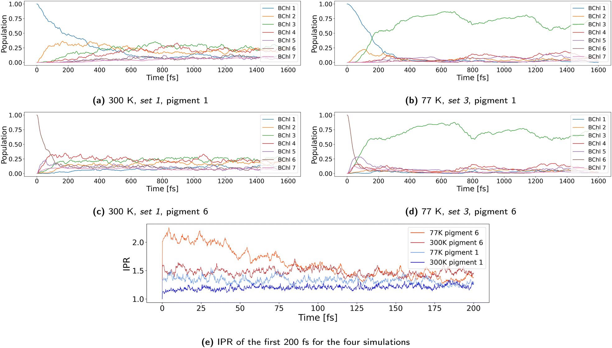 | ||
| Fig. 17 Averaged diabatic populations of the pigments during the 100 NAMD simulations of set 1 and set 3 with λ = 35 meV, scaled but not screened couplings and the exciton initially localized at pigment 1 or 6. (a) Trajectories of set 1 with our default settings at 300 K and initial occupation of pigment 1 and (c) pigment 6. (b) Trajectories of set 3 with the exciton being initially localized at pigment 1 and (d) pigment 6. (e) The IPR of the four simulations shown above, each averaged over the 100 NAMD trajectories. | ||
The two paths from pigment 1 via pigment 2 to pigment 3 or from pigment 6 via 5 and 4 to pigment 3 do not change with temperature. In both cases, the transfer to pigment 3 is faster at 77 K than at 300 K (Fig. 17). Furthermore, after 500 fs, pigment 3 reaches twice the population at 77 K than at 300 K, indicating localization at the lowest energy pigment. The energy is rapidly dissipated to the environment and the exciton relaxes to the lowest energy state where it is trapped because of the reduced fluctuations of the site energies. Both findings, faster transport to pigment 3 and higher localization there, agree with ref. 125. The reason for the faster transport to the final pigment 3 is the higher delocalization during the first femtoseconds at 77 K. Comparing the IPR averaged over 100 NAMD simulations for the first 200 fs in Fig. 17e, the trend becomes obvious. Furthermore, the transport to pigment 3 is slightly faster if the exciton is initially located on pigment 6. This can be explained by the higher delocalization of the pigments along this pathway, too. The population decay of pigment 6 is shown for a single trajectory as an example in the ESI† (Fig. S38) and is compared to the trajectory using the same starting structure but having pigment 1 initially occupied. There, the larger delocalization in the first 100 fs for the initially occupied pigment 6 can be seen well.
After the ≈500 fs of simulation, the picture changes completely and a contradiction to the previous findings becomes apparent. The average delocalization at 77 K reduces over time and finally remains at a lower value than the average delocalization at 300 K. The reason for the high localization at 77 K is the stabilization of the exciton on pigment 3 alone, which is energetically isolated. While site energy fluctuations cause frequent changes in the site energy ladder at 300 K, the fluctuations of site energies and couplings in MD simulations are reduced by 50% at 77 K (see Fig. S6 and S9 in the ESI†) compared to the fluctuations at 300 K (see Fig. S4, S5, S7 and S8 in the ESI†). This observed reduction in the fluctuations nicely agrees with the fact that the fluctuations scale with the square root of the temperature. The reduced fluctuations lead to more pronounced trapping in the lowest energy state, which is pigment 3 in this case.
Tables 3 and 5 compare the averaged IPR values and show the higher localization at 77 K, but the differences are small. For example, for propagations with 65 meV reorganization energy as well as scaled and screened couplings, a delocalization over 1.05 pigments is found. At 300 K the corresponding IPR is 1.15. The default settings at 300 K (35 meV, scaling, no screening) lead to IPRs of 1.37 and 1.38, for set1 and set 2, respectively. At 77 K, we found slightly lower values of around 1.30 (see Tables 3 and 5). The IPR is of the same magnitude in all four sets, and so it does not depend on the initial structure. We interpret this as a logical consequence of a hopping transport in the Marcus regime, which becomes more localized at lower temperatures.
| set 3 | set 6 | set 7 | set 8 | set 3, pigment 6 | |
|---|---|---|---|---|---|
| λ = 35 meV, scaled couplings | 1.34 | 1.26 | 1.27 | 1.23 | 1.35 |
| λ = 65 meV, scaled and screened couplings | 1.06 | 1.03 | 1.06 | 1.05 | 1.07 |
In addition to localization, the transfer rate of exciton transport in the Marcus regime decreases slightly at lower temperatures, because of the factor of exp(−1/T).126 To analyze the speed of the exciton during the whole simulation time, Fig. S41 in the ESI,† visualizes the number of hops within 100 propagation runs. Compared to 300 K the number of hops is reduced in all sets of 77 K, meaning that the speed of the exciton in general decreases at lower temperature. The fact that these hops are frequent in set 8 is not due to the couplings there (they are in the same order of magnitude as in the other sets, see Fig. S9, ESI†), but due to the fact that the energies cross more often, as can be seen in Fig. S6 in the ESI.†
In summary, we observed faster initial transport at 77 K due to higher delocalization at the first 200 fs. The average localization is independent of the starting structure. On the other hand, the transport pathway and the final pigment that is occupied most of the time depend on the starting structure, due to smaller thermal fluctuations of the site energies. This is in agreement with recent findings reported by Duan et al.22 They studied the low temperature dynamics of excitons in FMO using a Frenkel Hamlitonian and spectral density fitted to the experimental data. They reported an ultrafast transfer between sites 1 and 2 within about 200 fs, which is in line with our simulations. A slightly slower transfer to site 3 is reported, which may be a particular feature of the Hamiltonian.23,98 Furthermore, a weak temperature dependence of the transfer rates is reported, slightly slowing down with increasing temperature, as also seen in our simulations.
Reorganization energies are of particular interest, since they can slow down the propagation significantly, as pointed out by Duan et al.22 Interestingly, their measurements lead to an estimate of about 15 meV, much smaller than the parameter ranges sampled in our simulations, where we have values for the inner-sphere reogranization energy between 35 and 65 meV and an outer-sphere contribution of about 20 meV explicitly covered by the QM/MM interactions. Therefore, our reorganization energy per site is more than 2–3 times higher than the experimental estimate. Note, however, that this is the reorganization energy applicable for a localized transfer. For delocalized excitons, it is reduced by |an|2 accoding to eqn (9). For instance, if an exciton is delocalized over two sites, this would reduce the reorganization energy per site by 50%, which already can rationalize the difference between the theoretical values and experimental estimates. Although we find an average delocalization of about 1.3 depending on parameters used (Table 3), inspection of the trajectories reported above shows that in many runs the initial dynamics is quite fast showing a delocalization over several sites.
5 Conclusion
In this study, we applied a NAMD multiscale-method to simulate the exciton propagation within the FMO complex. The employed methodology is based on surface hopping and classical nuclear dynamics. This work shows that a sufficiently accurate representation of the electronic structure and the coupling to the fluctuating electrostatic environment via a QM/MM algorithm provides insights into the reason for the efficiency and the underlying mechanisms promoting this efficient exciton transfer, as detailed in the Introduction. Due to the large size of the system, the relatively long time-scale and the large number of trajectories to be computed, and the fact that we compute the crucial parameters for the electronic structure ‘on the fly’ along these trajectories, we have to introduce approximations into the electronic structure calculations. The efficiency of the method allowing for extensive sampling results from (i) fragmentation of the electronic system, (ii) using a semi-empirical DFT (LC-DFTB2) method to compute reference data for a large training data set and (iii) training an NN on this data set, which allows computing all relevant electronic parameters ‘on the fly’. In total, we performed 100 NAMD simulations of 10 ps length to achieve converged statistics for every single combination of parameters (temperature, scaling factor for couplings, reorganization energy, etc.).Testing of methods is a crucial step and ensuring that correct results are computed for the right reason is essential for the interpretability of the results. This is in particular important for the present system, since standard DFT methods can be deficient in computing excitonic couplings and reorganization energies. Therefore, even if it would not be computationally prohibitive, a straightforward application of a DFT-based NAMD simulation may not guarantee a correct outcome. The fragmentation of the system and the computation of parameters like site energies and their fluctuations, excitonic couplings and reorganization energies, which are the key ingredients of our method, allow systematically accessing the reliability of the approach. In particular, the fragmentation approach enables computing all critical values from ab initio methods (or reasonable approximate quantum chemical models) on the one hand, but also allows improving these parameters in cases where doubts about the accuracy even of ab initio methods persist. We have therefore studied a range of values using reasonable lower and upper bounds, and systematically tested their impact. In sum, we have shown (i) that the site energies are in a reasonable range of values, comparable to other approaches, (ii) that the choice of reorganization energy is critical and has to be carefully assessed and (iii) that some uncertainty still exists in the excitonic couplings, which have a moderate influence on the dynamics. Furthermore, (iv) the site energy fluctuations seem to be captured correctly as can be estimated from the computed spectral density, while (v) the fluctuations of the couplings seem to be of minor importance, since they can be substituted by their averages without large changes in the results. Moreover, it is remarkable that the NN is able to learn the electrostatic interactions with such an accuracy, since the energy difference between the sites is just a couple of 10 meV.
As discussed in the Introduction, the exciton transfer in FMO is surprisingly fast, and the transfer from site 1 or 6 to site 3 covers a distance of several nanometers within a picosecond, which is on the same time-scale as many ultrafast photo-chemical events like the isomerization of retinal. Based on classical nuclear dynamics, the energy funnel results completely from the electrostatic tuning of the chromophores. Our simulations show a fast decay within 1 ps to the lowest energy states, therefore confirming earlier proposals that the efficiency is not based on special quantum effects, whether electronic or nuclear. Rather, it can be attributed to the unusual molecular properties of the BChl pigments.
Chlorophyll seems to be designed not to respond significantly to the environmental electrostatics. This fact is apparent, e.g., in a comparison to the retinal chromophore in retinal proteins, where electrostatic tuning is at least an order of magnitude larger, allowing this molecule to absorb in the whole visible spectrum depending on the protein environment.33 As a consequence of the small electrostatic tuning of BChl in FMO (of about 0.04 eV), the driving force for the energy transfer is rather small, but sufficient to funnel the excitons from sites 1/6 to site 3, where the exciton can be further transferred to the reaction center. The reason for the efficient transfer instead can be traced back to the reorganization energy. The tiny change in dipole moment upon excitation of BChl (1–2 D)84 leads to a low outer sphere reorganization energy (about 0.021 eV). Also the inner sphere contribution is very small (about 0.035 eV).
For organic materials a very efficient charge transfer mechanism has been described and termed 'transient localization theory' (TLT),67,68 which has been recovered for exciton transfer as well.64,71 Here, transfer efficiency and delocalization are clearly related. For |Hmn| ≈ λ/2, the localized hopping picture breaks down, and delocalization becomes an important factor promoting the efficiency of the transport. Interestingly, since couplings in FMO are rather small (scaled <0.02 eV) and disorder is high, a hopping picture could be expected. The surprising fact is that the comparably tiny reorganization energy still allows partial delocalization. This surprising property of BChl is best appreciated in comparison to organic materials: there, reorganization energies are between 0.2 and 0.5 eV, while the couplings are on the order of 0.1 eV.
For the parameter values found in FMO, the exciton transfer mechanism is at a boundary between localized hopping and delocalized band-like transfer, manifesting itself in the small IPR below 2. While a Marcus type picture is no more applicable in this regime on the one hand87,127 a band-structure type description cannot be assumed since the coupling between the sites is too small compared to the fluctuations of the site energies, which leads to a rapidly fluctuating picture of adiabatic states as shown in Fig. S48 (ESI†). The analysis of single trajectories shows events where exciton localization on one site and delocalized fast transfer alternate. The route starting at site 1 seems to lead to a slightly more localized exciton than the route starting at site 6.
This finding agrees with results of ref. 22 and 34, where it was reported that no long-range coherent transport is necessary to account for the efficient transfer at low temperatures as well as at 300 K. Furthermore, the experimental data also do not favor a strongly delocalized exciton. The relatively high reorganization energy reported in ref. 22 compared to previous FMO studies suggests a partially localized excitation, similar to that found in our simulations. Thermal relaxation after photo-excitation seems to be the main mechanism to be consistent with these recent experimental findings. Such a mechanism is surely at work in our NAMD simulations, leading to the exciton distribution at 300 K, which is much sharpened at low temperatures.
Conflicts of interest
There are no conflicts to declare.Acknowledgements
The authors gratefully acknowledge support from the German Research Foundation (DFG) through the joint grant EL 206/18-1 and KL-1299/18-1, through the grant KL-1299/24-1 and through the Research Training Groups 2039 (M. S., D. S. H. and M. E.) and 2450 (P. M. D., M. K. and M. E.). M. S. and M. E. are also thankful for financial support from the Klaus Tschira Stiftung through SIMPLAIX. Furthermore, part of the simulations were performed on a computing cluster funded through the project INST 676/7-1 FUGG. The authors acknowledge support from the state of Baden-Württemberg through bwHPC and the German Research Foundation (DFG) through grant no. INST 40/575-1 FUGG (JUSTUS 2 cluster).References
- S. J. Jang and B. Mennucci, Rev. Mod. Phys., 2018, 90, 035003 CrossRef CAS.
- R. E. Fenna and B. W. Matthews, Nature, 1975, 258, 573–577 CrossRef CAS.
- S. Savikhin, D. R. Buck and W. S. Struve, Chem. Phys., 1997, 223, 303–312 CrossRef CAS.
- G. S. Engel, T. R. Calhoun, E. L. Read, T.-K. Ahn, T. Mančal, Y.-C. Cheng, R. E. Blankenship and G. R. Fleming, Nature, 2007, 446, 782–786 CrossRef CAS PubMed.
- P. Rebentrost, M. Mohseni and A. Aspuru-Guzik, J. Phys. Chem. B, 2009, 113, 9942–9947 CrossRef CAS PubMed.
- D. M. Wilkins and N. S. Dattani, J. Chem. Theory Comput., 2015, 11, 3411–3419 CrossRef CAS PubMed.
- F. Caruso, A. W. Chin, A. Datta, S. F. Huelga and M. B. Plenio, Phys. Rev. A: At., Mol., Opt. Phys., 2010, 81, 062346 CrossRef.
- M. Sarovar, A. Ishizaki, G. R. Fleming and K. B. Whaley, Nat. Phys., 2010, 6, 462–467 Search PubMed.
- M. Tiersch, S. Popescu and H. J. Briegel, Philos. Trans. R. Soc. A, 2012, 370, 3771–3786 CrossRef PubMed.
- J. T. Nielsen, N. V. Kulminskaya, M. Bjerring, J. M. Linnato, M. Rätsep, M. O. Pedersen, P. H. Lambrev, M. Dorogi, G. Garab, K. Thomsen, C. Jegerschöld, N.-U. Frigaard, M. Lindahl and N. C. Nielsen, Nat. Commun., 2016, 7, 12454 CrossRef CAS PubMed.
- M. Schmidt am Busch, F. Müh, M. E. Madjet and T. Renger, J. Phys. Chem. Lett., 2011, 2, 93–98 CrossRef CAS PubMed.
- J.-H. Chen, H. Wu, C. Xu, X.-C. Liu, Z. Huang, S. Chang, W. Wang, G. Han, T. Kuang, J.-R. Shen and X. Zhang, Science, 2020, 370, 931–938 Search PubMed.
- H. Li, S. Jubelirer, A. M. G. Costas, N.-U. Frigaard and D. A. Bryant, Arch. Microbiol., 2009, 191, 853–867 CrossRef CAS PubMed.
- S. Savikhin and W. Struve, Biochemistry, 1994, 33, 11200–11208 CrossRef CAS PubMed.
- S. I. E. Vulto, A. M. Streltsov and T. J. Aartsma, J. Phys. Chem. B, 1997, 101, 4845–4850 CrossRef CAS.
- E. M. Franken, S. Neerken, R. J. W. Louwe, J. Amesz and T. J. Aartsma, Biochemistry, 1998, 37, 5046–5051 CrossRef CAS PubMed.
- T. Brixner, J. Stenger, H. M. Vaswani, M. Cho, R. E. Blankenship and G. R. Fleming, Nature, 2005, 434, 625–628 CrossRef CAS PubMed.
- E. Thyrhaug, K. Zidek, J. Dostal, D. Bina and D. Zigmantas, J. Phys. Chem. Lett., 2016, 7, 1653–1660 CrossRef CAS PubMed.
- J. Dostál, J. Pšenčík and D. Zigmantas, Nat. Chem., 2016, 8, 705–710 CrossRef PubMed.
- T. Reinot, A. Khmelnitskiy, A. Kell, M. Jassas and R. Jankowiak, ACS Omega, 2021, 6, 5990–6008 CrossRef CAS PubMed.
- J. S. Higgins, L. T. Lloyd, S. H. Sohail, M. A. Allodi, J. P. Otto, R. G. Saer, R. E. Wood, S. C. Massey, P.-C. Ting, R. E. Blankenship and G. S. Engel, Proc. Natl. Acad. Sci. U. S. A., 2021, 118, 2018240118 CrossRef PubMed.
- H.-G. Duan, A. Jha, L. Chen, V. Tiwari, R. J. Cogdell, K. Ashraf, V. I. Prokhorenko, M. Thorwart and R. J. D. Miller, Proc. Natl. Acad. Sci. U. S. A., 2022, 119, 2212630119 CrossRef PubMed.
- J. Adolphs and T. Renger, Biophys. J., 2006, 91, 2778–2797 CrossRef CAS PubMed.
- M. T. W. Milder, B. Brüggemann, R. van Grondelle and J. L. Herek, Photosynth. Res., 2010, 104, 257–274 CrossRef CAS PubMed.
- C. Olbrich, T. L. C. Jansen, J. Liebers, M. Aghtar, J. Strümpfer, K. Schulten, J. Knoester and U. Kleinekathöfer, J. Phys. Chem. B, 2011, 115, 8609–8621 CrossRef CAS PubMed.
- S. Jurinovich, C. Curutchet and B. Mennucci, ChemPhysChem, 2014, 15, 3194–3204 CrossRef CAS PubMed.
- X. Jia, J. Mei, J. Z. H. Zhang and Y. Mo, Sci. Rep., 2015, 5, 17096 CrossRef CAS PubMed.
- S. Maity and U. Kleinekathöfer, Photosynth. Res., 2023, 156, 147–162 CrossRef CAS PubMed.
- S. Saito, M. Higashi and G. R. Fleming, J. Phys. Chem. B, 2019, 123, 9762–9772 CrossRef CAS PubMed.
- H. W. Kim, A. Kelly, J. W. Park and Y. M. Rhee, J. Am. Chem. Soc., 2012, 134, 11640–11651 CrossRef CAS PubMed.
- E. Rivera, D. Montemayor, M. Masia and D. F. Coker, J. Phys. Chem. B, 2013, 117, 5510–5521 CrossRef CAS PubMed.
- F. Häse, S. Valleau, E. Pyzer-Knapp and A. Aspuru-Guzik, Chem. Sci., 2016, 7, 5139–5147 RSC.
- B. M. Bold, M. Sokolov, S. Maity, M. Wanko, P. M. Dohmen, J. J. Kranz, U. Kleinekathöfer, S. Höfener and M. Elstner, Phys. Chem. Chem. Phys., 2020, 22, 10500–10518 RSC.
- H.-G. Duan, V. I. Prokhorenko, R. J. Cogdell, K. Ashraf, A. L. Stevens, M. Thorwart and R. J. D. Miller, Proc. Natl. Acad. Sci. U. S. A., 2017, 114, 8493–8498 CrossRef CAS PubMed.
- J. Cao, R. J. Cogdell, D. F. Coker, H.-G. Duan, J. Hauer, U. Kleinekathöfer, T. L. C. Jansen, T. Mančal, R. J. D. Miller, J. P. Ogilvie, V. I. Prokhorenko, T. Renger, H.-S. Tan, R. Tempelaar, M. Thorwart, E. Thyrhaug, S. Westenhoff and D. Zigmantas, Sci. Adv., 2020, 6, aaz4888 CrossRef PubMed.
- J. E. Runeson, J. E. Lawrence, J. R. Mannouch and J. O. Richardson, J. Phys. Chem. Lett., 2022, 13, 3392–3399 CrossRef CAS PubMed.
- K. H. Cho and Y. M. Rhee, Phys. Chem. Chem. Phys., 2021, 23, 26623–26639 RSC.
- E. Cignoni, V. Slama, L. Cupellini and B. Mennucci, J. Chem. Phys., 2022, 156, 120901 CrossRef CAS PubMed.
- T. Renger, M.-A. Madjet, M. Schmidt am Busch, J. Adolphs and F. Müh, Photosynth. Res., 2013, 116, 367–388 CrossRef CAS PubMed.
- C. P. van der Vegte, J. D. Prajapati, U. Kleinekathöfer, J. Knoester and T. L. C. Jansen, J. Phys. Chem. B, 2015, 119, 1302–1313 CrossRef CAS PubMed.
- R. Crespo-Otero and M. Barbatti, Chem. Rev., 2018, 118, 7026–7068 CrossRef CAS PubMed.
- S. Mai, P. Marquetand and L. González, Quantum Chemistry and Dynamics of Excited States: Methods and Applications, John Wiley & Sons Ltd, 2021, ch. 16 Search PubMed.
- J. M. Toldo, M. T. do Casal, E. Ventura, S. A. do Monte and M. Barbatti, Phys. Chem. Chem. Phys., 2023, 25, 8293–8316 RSC.
- D. V. Cofer-Shabica, M. F. S. Menger, Q. Ou, Y. Shao, J. E. Subotnik and S. Faraji, J. Chem. Theory Comput., 2022, 18, 4601–4614 CrossRef CAS PubMed.
- M. Bondanza, B. Demoulin, F. Lipparini, M. Barbatti and B. Mennucci, J. Phys. Chem. A, 2022, 126, 6780–6789 CrossRef CAS PubMed.
- D. Avagliano, E. Lorini and L. González, Philos. Trans. R. Soc. A, 2022, 380, 20200381 CrossRef PubMed.
- L. Wang, J. Qiu, X. Bai and J. Xu, Wiley Interdiscip. Rev.: Comput. Mol. Sci., 2019, 10, e1435 Search PubMed.
- A. Sisto, C. Stross, M. W. van der Kamp, M. OConnor, S. McIntosh-Smith, G. T. Johnson, E. G. Hohenstein, F. R. Manby, D. R. Glowacki and T. J. Martinez, Phys. Chem. Chem. Phys., 2017, 19, 14924–14936 RSC.
- S. Mukherjee, M. Pinheiro, B. Demoulin and M. Barbatti, Philos. Trans. R. Soc. A, 2022, 380, 20200382 CrossRef PubMed.
- T. Kubař and M. Elstner, J. Phys. Chem. B, 2010, 114, 11221–11240 CrossRef PubMed.
- T. Kubař and M. Elstner, J. R. Soc., Interface, 2013, 10, 20130415 CrossRef PubMed.
- T. Kubař and M. Elstner, Phys. Chem. Chem. Phys., 2013, 15, 5794–5813 RSC.
- G. Lüdemann, P. B. Woiczikowski, T. Kubař, M. Elstner and T. B. Steinbrecher, J. Phys. Chem. B, 2013, 117, 10769–10778 CrossRef PubMed.
- G. Lüdemann, I. A. Solov'yov, T. Kubař and M. Elstner, J. Am. Chem. Soc., 2015, 137, 1147–1156 CrossRef PubMed.
- T. Kubař, M. Elstner and Q. Cui, Annu. Rev. Biophys., 2023, 52, 525–551 CrossRef PubMed.
- A. Heck, J. J. Kranz, T. Kubař and M. Elstner, J. Chem. Theory Comput., 2015, 11, 5068–5082 CrossRef CAS PubMed.
- A. Heck, J. J. Kranz and M. Elstner, J. Chem. Theory Comput., 2016, 12, 3087–3096 CrossRef CAS PubMed.
- R. Haldar, M. Kozlowska, M. Ganschow, S. Ghosh, M. Jakoby, H. Chen, F. Ghalami, W. Xie, S. Heidrich, Y. Tsutsui, J. F. S. Seki, I. Howard, B. S. Richards, U. H. Bunz, M. Elstner, W. Wenzel and C. Wöll, Chem. Sci., 2021, 12, 4477–4483 RSC.
- M. Krämer, P. M. Dohmen, W. Xie, D. Holub, A. S. Christensen and M. Elstner, J. Chem. Theory Comput., 2020, 16, 4061–4070 CrossRef PubMed.
- W. Xie, D. Holub, T. Kubař and M. Elstner, J. Chem. Theory Comput., 2020, 16, 2071–2084 CrossRef CAS PubMed.
- S. Roosta, F. Ghalami, M. Elstner and W. Xie, J. Chem. Theory Comput., 2022, 18, 1264–1274 CrossRef CAS PubMed.
- P. M. Dohmen, M. Krämer, P. Reiser, P. Friederich, M. Elstner and W. Xie, J. Chem. Theory Comput., 2023, 19, 3825–3838 CrossRef CAS PubMed.
- J. J. Kranz and M. Elstner, J. Chem. Theory Comput., 2016, 12, 4209–4221 CrossRef CAS PubMed.
- S. Giannini, W.-T. Peng, L. Cupellini, D. Padula, A. Carof and J. Blumberger, Nat. Commun., 2022, 13, 2755 CrossRef CAS PubMed.
- M. F. S. J. Menger, F. Plasser, B. Mennucci and L. González, J. Chem. Theory Comput., 2018, 14, 6139–6148 CrossRef CAS PubMed.
- S. Mukamel, J. Phys. Chem. A, 2013, 117, 10563–10564 CrossRef CAS PubMed.
- S. Fratini, S. Ciuchi, D. Mayou, G. T. de Laissardière and A. Troisi, Nat. Mater., 2017, 16, 998–1002 CrossRef CAS PubMed.
- S. Ciuchi, S. Fratini and D. Mayou, Phys. Rev. B: Condens. Matter Mater. Phys., 2011, 83, 081202 CrossRef.
- S. Giannini, A. Carof, M. Ellis, H. Yang, O. G. Ziogos, S. Ghosh and J. Blumberger, Nat. Commun., 2019, 10, 3843 CrossRef PubMed.
- S. Giannini and J. Blumberger, Acc. Chem. Res., 2022, 55, 819–830 CrossRef CAS PubMed.
- A. J. Sneyd, T. Fukui, D. Paleček, S. Prodhan, I. Wagner, Y. Zhang, J. Sung, S. M. Collins, T. J. A. Slater, Z. Andaji-Garmaroudi, L. R. MacFarlane, J. D. Garcia-Hernandez, L. Wang, G. R. Whittell, J. M. Hodgkiss, K. Chen, D. Beljonne, I. Manners, R. H. Friend and A. Rao, Sci. Adv., 2021, 7, eabh4232 CrossRef CAS PubMed.
- P. B. Woiczikowski, T. Steinbrecher, T. Kubař and M. Elstner, J. Phys. Chem. B, 2011, 115, 9846–9863 CrossRef CAS PubMed.
- D. Holub, H. Ma, N. Krauß, T. Lamparter, M. Elstner and N. Gillet, Chem. Sci., 2018, 9, 1259–1272 RSC.
- E. Sjulstok, G. Lüdemann, T. Kubař, M. Elstner and I. A. Solov'yov, Biophys. J., 2018, 114, 2563–2572 CrossRef CAS PubMed.
- D. Holub, T. Kubař, T. Mast, M. Elstner and N. Gillet, Phys. Chem. Chem. Phys., 2019, 21, 11956–11966 RSC.
- D. Holub, T. Lamparter, M. Elstner and N. Gillet, Phys. Chem. Chem. Phys., 2019, 21, 17072–17081 RSC.
- H. M. Senn and W. Thiel, Angew. Chem., Int. Ed., 2009, 48, 1198–1229 CrossRef CAS PubMed.
- P.-A. Plötz, T. Niehaus and O. Kühn, J. Chem. Phys., 2014, 140, 174101 CrossRef PubMed.
- N. Schieschke, B. M. Bold, P. M. Dohmen, D. Wehl, M. Hoffmann, A. Dreuw, M. Elstner and S. Höfener, J. Comput. Chem., 2021, 42, 1402–1418 CrossRef CAS PubMed.
- J. J. Kranz, M. Elstner, B. Aradi, T. Frauenheim, V. Lutsker, A. D. Garcia and T. A. Niehaus, J. Chem. Theory Comput., 2017, 13, 1737–1747 CrossRef CAS PubMed.
- M. Sokolov, B. M. Bold, J. J. Kranz, S. Höfener, T. A. Niehaus and M. Elstner, J. Chem. Theory Comput., 2021, 17, 2266–2282 CrossRef CAS PubMed.
- J. C. Tully, J. Chem. Phys., 1990, 93, 1061–1071 CrossRef CAS.
- M. Rätsep, Z.-L. Cai, J. R. Reimers and A. Freiberg, J. Chem. Phys., 2011, 134, 024506 CrossRef PubMed.
- M. Higashi, T. Kosugi, S. Hayashi and S. Saito, J. Phys. Chem. B, 2014, 118, 10906–10918 CrossRef CAS PubMed.
- A. Troisi, Org. Electron., 2011, 12, 1988–1991 CrossRef CAS.
- D. V. Matyushov, Phys. Chem. Chem. Phys., 2023, 25, 7589–7610 RSC.
- H. Oberhofer, K. Reuter and J. Blumberger, Chem. Rev., 2017, 117, 10319–10357 CrossRef CAS PubMed.
- A. Damjanović, I. Kosztin, U. Kleinekathöfer and K. Schulten, Phys. Rev. E: Stat., Nonlinear, Soft Matter Phys., 2002, 65, 031919 CrossRef PubMed.
- M. J. Abraham, T. Murtola, R. Schulz, S. Páll, J. C. Smith, B. Hess and E. Lindahl, SoftwareX, 2015, 1, 19–25 CrossRef.
- S. Páll, M. J. Abraham, C. Kutzner, B. Hess and E. Lindahl, Solving Software Challenges for Exascale, Cham, 2015, pp. 3–27 Search PubMed.
- H. J. C. Berendsen, D. van der Spoel and R. van Drunen, Comput. Phys. Commun., 1995, 91, 43–56 CrossRef CAS.
- S. Nosé, Mol. Phys., 1984, 52, 255–268 CrossRef.
- W. G. Hoover, Phys. Rev. A: At., Mol., Opt. Phys., 1985, 31, 1695–1697 CrossRef PubMed.
- M. Parrinello and A. Rahman, J. Appl. Phys., 1981, 52, 7182–7190 CrossRef CAS.
- S. Nosé and M. L. Klein, Mol. Phys., 1983, 50, 1055–1076 CrossRef.
- C. Olbrich, J. Stümpfer, K. Schulten and U. Kleinekathöfer, J. Phys. Chem. B, 2011, 115, 758–764 CrossRef CAS PubMed.
- A. Sali and T. L. Blundell, J. Mol. Biol., 1993, 234, 779–815 CrossRef CAS PubMed.
- P. Nalbach, D. Braun and M. Thorwart, Phys. Rev. E: Stat., Nonlinear, Soft Matter Phys., 2011, 84, 041926 CrossRef CAS PubMed.
- S. Maity, B. Bold, J. Prajapati, M. Sokolov, T. Kubar, M. Elstner and U. Kleinekathöfer, J. Phys. Chem. Lett., 2020, 11, 8660–8667 CrossRef CAS PubMed.
- T. Yanai, D. P. Tew and N. C. Handy, Chem. Phys. Lett., 2004, 393, 51–57 CrossRef CAS.
- S. Höfener, J. Comput. Chem., 2014, 35, 1716–1724 CrossRef PubMed.
- A. D. Becke, J. Chem. Phys., 1993, 98, 5648 CrossRef CAS.
- C. Lee, W. Yang and R. G. Parr, Phys. Rev. B: Condens. Matter Mater. Phys., 1988, 37, 785 CrossRef CAS PubMed.
- P. J. Stephens, F. J. Delvin, C. F. Chabalowski and M. J. Frisch, J. Phys. Chem., 1994, 98, 11623 CrossRef CAS.
- M. J. Frisch, G. W. Trucks, H. B. Schlegel, G. E. Scuseria, M. A. Robb, J. R. Cheeseman, G. Scalmani, V. Barone, B. Mennucci, G. A. Petersson, H. Nakatsuji, M. Caricato, X. Li, H. P. Hratchian, A. F. Izmaylov, J. Bloino, G. Zheng, J. L. Sonnenberg, M. Hada, M. Ehara, K. Toyota, R. Fukuda, J. Hasegawa, M. Ishida, T. Nakajima, Y. Honda, O. Kitao, H. Nakai, T. Vreven, J. A. M. Jr., J. E. Peralta, F. Ogliaro, M. Bearpark, J. J. Heyd, E. Brothers, K. N. Kudin, V. N. Staroverov, R. Kobayashi, J. Normand, K. Raghavachari, A. Rendell, J. C. Burant, S. S. Iyengar, J. Tomasi, M. Cossi, N. Rega, J. M. Millam, M. Klene, J. E. Knox, J. B. Cross, V. Bakken, C. Adamo, J. Jaramillo, R. Gomperts, R. E. Stratmann, O. Yazyev, A. J. Austin, R. Cammi, C. Pomelli, J. W. Ochterski, R. L. Martin, K. Morokuma, V. G. Zakrzewski, G. A. Voth, P. Salvador, J. J. Dannenberg, S. Dapprich, A. D. Daniels, O. Farkas, J. B. Foresman, J. V. Ortiz, J. Cioslowski and D. J. Fox, Gaussian 09, Revision A.02, 2009 Search PubMed.
- C. Brückner and B. Engels, J. Comput. Chem., 2016, 37, 1335–1344 CrossRef PubMed.
- R. S. Knox and B. Q. Spring, Photochem. Photobiol., 2003, 77, 497–501 CrossRef CAS PubMed.
- M. E. Madjet, A. Abdurahman and T. Renger, J. Phys. Chem. B, 2006, 110, 17268–17281 CrossRef CAS PubMed.
- G. D. Scholes, C. Curutchet, B. Mennucci, R. Cammi and J. Tomasi, J. Phys. Chem. B, 2007, 111, 6978–6982 CrossRef CAS PubMed.
- M. Wanko, M. Hoffmann, P. Strodel, A. Koslowski, W. Thiel, F. Neese, T. Frauenheim and M. Elstner, J. Phys. Chem. B, 2005, 109, 3606–3615 CrossRef CAS PubMed.
- M. Wanko, M. Hoffmann, J. Frähmcke, T. Frauenheim and M. Elstner, J. Phys. Chem. B, 2008, 112, 11468–11478 CrossRef CAS PubMed.
- M. L. Chaillet, F. Lengauer, J. Adolphs, F. Müh, A. S. Fokas, D. J. Cole, A. W. Chin and T. Renger, J. Phys. Chem. Lett., 2020, 11, 10306–10314 CrossRef CAS PubMed.
- J. Gao, W. Shi, J. Ye, X. Wang, H. Hirao and Y. Zhao, J. Phys. Chem. B, 2013, 117, 3488–3495 CrossRef CAS PubMed.
- S. Shim, P. Rebentrost, S. Valleau and A. Aspuru-Guzik, Biophys. J., 2012, 102, 649–660 CrossRef CAS PubMed.
- X. Lu and R. M. Pearlstein, Photochem. Photobiol., 1993, 57, 86–91 CrossRef CAS.
- D. Gülen, J. Phys. Chem., 1996, 100, 17683–17689 CrossRef.
- R. J. W. Louwe, J. Vrieze, A. J. Hoff and T. J. Aartsma, J. Phys. Chem. B, 1997, 101, 11280–11287 CrossRef CAS.
- S. I. E. Vulto, M. A. de Baat, R. J. W. Louwe, H. P. Permentier, T. Neef, M. Miller, H. van Amerongen and T. J. Aartsma, J. Phys. Chem. B, 1998, 102, 9577–9582 CrossRef CAS.
- M. Wendling, M. A. Przyjalgowski, D. Gülen, S. I. E. Vulto, T. J. Aartsma, R. van Grondelle and H. van Amerogen, Photosynth. Res., 2002, 71, 99–123 CrossRef CAS PubMed.
- C. Curutchet and B. Mennucci, Chem. Rev., 2017, 117, 294–343 CrossRef CAS PubMed.
- B. M. Bold, M. Sokolov, S. Maity, M. Wanko, P. M. Dohmen, J. J. Kranz, U. Kleinekathöfer, S. Höfener and M. Elstner, Phys. Chem. Chem. Phys., 2023, 25, 22535–22537 RSC.
- M. Gaus, A. Goez and M. Elstner, J. Chem. Theory Comput., 2013, 9, 338–354 CrossRef CAS PubMed.
- T. Kubař and M. Elstner, J. Phys. Chem. B, 2009, 113, 5653–5656 CrossRef PubMed.
- M. Aghtar, J. Strümpfer, C. Olbrich, K. Schulten and U. Kleinekathöfer, J. Phys. Chem. B, 2013, 117, 7157–7163 CrossRef CAS PubMed.
- A. Ishizaki and G. R. Fleming, Proc. Natl. Acad. Sci. U. S. A., 2009, 106, 17255–17260 CrossRef PubMed.
- R. A. Marcus, J. Chem. Phys., 2004, 24, 966–978 CrossRef.
- A. Troisi, Chem. Soc. Rev., 2011, 40, 2347–2358 RSC.
Footnote |
| † Electronic supplementary information (ESI) available. See DOI: https://doi.org/10.1039/d4cp02116a |
| This journal is © the Owner Societies 2024 |