One- and two-photon absorption spectra of organoboron complexes: vibronic and environmental effects

Abstract

We synthesized a series of four parent aza-β-ketoiminate organoboron complexes and performed spectroscopic studies using both experimental and computational techniques. We studied how benzannulation influences the vibronic structure of the UV/Vis absorption bands with a focus on the bright lowest-energy π → π* electronic excitation. Theoretical simulations, accounting for inhomogeneous broadening effects using different embedding schemes, allowed gaining in-depth insights into the observed differences in band shapes induced by structural modifications. We observed huge variations in the distributions of vibronic transitions depending on the position of benzannulation. By and large, the harmonic approximation combined with the adiabatic hessian model delivers qualitatively correct band shapes for the one-photon absorption spectra, except in one case. We also assessed the importance of non-Condon effects (accounted for by the linear term in Herzberg–Teller expansion of the dipole moment) for S₀ → S₁ band shapes. It turned out that non-Condon contributions have no effect on the band shape in one-photon absorption spectra. In contrast, these effects significantly change the Franck–Condon band shapes of the two-photon absorption spectra. For one of the studied organoboron complexes we also performed a preliminary exploration of mechanical anharmonicity, resulting in an increase of the intensity of the 0–0 transition, which improves the agreement with the experimental data compared to the harmonic model.

---

1 Introduction

Medium-sized fluorescent organic molecules can penetrate through biological membranes, making them excellent candidates for bioimaging, including multiphoton microscopy techniques, provided the selected fluorophores exhibit sufficiently large multi-photon absorption cross sections.¹ The synthesis of such dyes is relatively straightforward, allowing to tailor their photophysical properties, solubility, and conjugation to specific molecules in live tissues by adding suitable functional groups. Additionally, such dyes can be integrated into various nanoparticles to boost their solubility in biological environments.² Organoboron complexes containing a BF₂ moiety, such as the well-known BODIPY derivatives, constitute a prominent class of fluorescent dyes owing their popularity to their excellent photophysical properties.³ Additionally, BODIPY derivatives have become highly popular in two-photon-based bioimaging and can be used, e.g., as amyloid markers.⁴ It is noteworthy that the photophysical properties of BODIPY dyes can be tuned by chemical modifications of their core. For instance, introducing an additional nitrogen atom, giving the aza-BODIPY core, increases the two-photon absorption (2PA) cross sections by up to 2000 GM (1 GM = 10⁻⁵⁰ cm⁴ s per photon) per molecule,⁵ while replacing the fluorine atoms linked to the boron center by hydrophilic groups increases water solubility.⁶ For comparison, we note that for a molecular probe the product of 2PA cross section and a fluorescence quantum yield larger than 50 GM is sufficient for bioimaging applications.¹ Similarly, dyes built with difluoroborane β-diiminate, difluoroborane β-diketonate, or difluoroborane β-ketoiminate groups have also been found to be effective 2PA biomarkers. In particular, BF₂-hydroxyiminates are widely used in bioimaging.^7–9 For example, a quadrupolar dye containing two N–BF₂–O groups was shown to present a 2PA cross section higher than 800 GM in the first biological window.¹⁰ Likewise, it was shown that introducing a double bond between the electron-donating aminophenyl group and the electron-accepting aza-β-ketoiminate (or amidate) moiety increases the 2PA cross section values by a factor of two.¹¹

Both the one- and two-photon absorption features of organic dyes can also be tuned by benzannulation of the central pyridyl ring in BF₂-carrying molecules. Depending on the position of the benzannulation one may observe either a blue- or redshift of the absorption band as demonstrated for a series of Pt(II) complexes.¹² Such auxochromic effects can be substantial, e.g., benzannulation can redshift the absorption band up to 121 nm.^13,14 Likewise, as recently shown by some of us, the emission efficiencies of quinoline derivatives presenting a BF₂ moiety differ significantly from their isoquinoline counterparts.^15,16 Clearly, varying the position of the benzo ring attached to the heterocyclic core is a viable route for controlling the photophysical properties.

The rigidity of the BF₂-heterocycle (or boraza derivatives of topology similar to phenantrene¹⁷) often induces a vibrational fine structure in the absorption/emission bands. For instance, a vibronic progression is found in the experimental UV/Vis spectra of solvated quinoline-, isoquinoline- (phenantrene-shaped), and phenantridine-based dyes.^15,16,18 Substitution and benzannulation potentially affect the intensity pattern of these vibronic transitions. Even though the experimental measurements are frequently accompanied by theoretical investigations of the vibronic effects, the latter typically rely on the harmonic approximation and neglect non-Condon effects. For small molecules (up to ca. 10 atoms) calculations taking into account anharmonic couplings are known to deliver very accurate spectra,^19–21 albeit at a high computational cost. A discussion of different approaches (variational and non-variational) to determine Franck–Condon factors (FCF) including anharmonicity can be found in ref. 22. Given the computational cost required to go beyond the harmonic approximation, the impact of mechanical anharmonicity on the vibronic structure of electronic bands of real-life fluorescent dyes is not well-established yet. Although the non-Condon contributions are expected to be trifling for bright one-photon (1PA) π → π* transitions, they can play an important role in the 2PA bandshapes, as shown for the 2PA spectra of fluorescent protein chromophores.^23–26

Given the huge potential of aza-β-ketoiminate-based (or amidate) fluorophores with a BF₂ moiety, we decided to perform an in-depth analysis of the vibrational fine structure of both 1PA and 2PA bands for the four newly synthesized compounds shown in Fig. 1. In more detail, the present work aims to: (i) analyze the influence of benzannulation on the vibronic structure; (ii) assess the importance of non-Condon effects for the band shapes in both 1PA and 2PA spectra; and (iii) pioneer the exploration of the role of mechanical anharmonicity on band shapes for medium-sized dyes. To compare the theoretical and experimental results, we additionally employ various embedding schemes to model the environment, combined with a recently developed machine learning (ML) approach.²⁷

Fig. 1 Studied compounds. See ESI† for IUPAC names.

2 Experimental section

The synthesis of dyes (illustrated for 1 in Fig. 2) was performed starting from amides as substrates in the same way as in the previous publication of some of the present authors.²⁸ The amides were obtained following a previously known procedure.²⁹ The structures of dyes were confirmed by NMR spectra (see ESI† file for NMR data, Fig. S1–S16).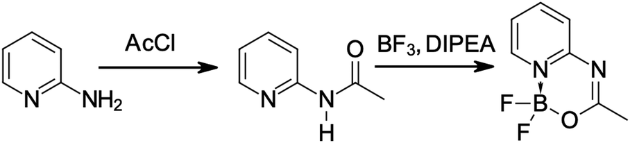

Fig. 2 Synthesis of compound 1. DIPEA and AcCl denote N,N-diisopropylethylamine and acetyl chloride, respectively. BF₃ was used as etherate.

3 Computational details

Vibronic-structure calculations

The vibrational reorganization energy,can be employed as a metric for selecting an adequate method for simulating vibrationally-resolved electronic spectra.^27,30 In this equation k labels the excited states, ω_j is the vibrational frequency and s^k_j is the Huang–Rhys factor related to the jth normal mode dimensionless displacement Δ^k_j between the electronic state k and the ground state minimum. In this work, we compute λ_vib using the vertical gradient (VG) potential energy surface (PES) model. This approach allows a cost-effective benchmarking of a set of 11 density functional approximations (DFAs) using the vibrational reorganization energy calculated with the cc-pVDZ atomic basis set³¹ as the metric and the wavefunction equation of motion coupled-cluster singles and doubles (EOM-CCSD) values as reference. The TD-DFT electronic structure calculations needed for computing λ_vib were achieved with Gaussian 16,³² applying the ultrafine pruned integration grid for the DFA calculations. In the calculations of vibrational reorganization energies using EOM-CCSD and DFAs solvent effects (chloroform) were accounted for using the polarizable continuum model (PCM) in its integral equation formalism (IEF) formulation.³³ The obtained results are listed in Table S1 in the ESI.† Several functionals give mean absolute percentage error (MAPE) for λ_vib with respect to the EOM-CCSD values smaller than 25%. We have decided to go for the LC-BLYP functional³⁴ in the following, except when explicitly noted. Indeed, on the one hand, this DFA is known to be very resistant to spurious oscillations in the profiles of high-order energy derivatives;^35,36 and, on the other hand, it provides reliable vibrational reorganization energies for a wide palette of BF₂-containing molecules.²⁷

In all subsequent vibronic-structure simulations, the ground and first electronic excited-state geometries were optimized at the LC-BLYP/cc-pVDZ level and the evaluations of the corresponding Hessians were next performed at the same level of theory. These calculations were achieved with Gaussian 16.³² It is noteworthy that a high-quality integration grid (250 radial shells, with 974 points per shell) was used to prevent spurious oscillations during anharmonic calculations (see below). All harmonic simulations were performed using the FCclasses 3 program.^37,38 Vibronic-structure calculations were achieved using the Adiabatic Hessian (AH)³⁹ PES model which employed the harmonic approximation. In the AH approach, one determines the Hessian in initial and final states at their respective minimum-energy geometries. In these simulations, we assumed a temperature of either 0 K or 298 K, as indicated in the “Results and Discussion” Section. We tested the results of the harmonic approximation using both the time-independent (TI)^40–43 approach (considering up to 10¹² transitions) and the time-dependent (TD)^44,45 approaches. In the TI approach, Franck–Condon integrals between vibrational wavefunctions in the initial and final electronic states are evaluated explicitly. This method can therefore be used for transition assignments. The often slow convergence of the TI approach can be overcome by using the TD approach which relies on the Fourier-transformation of the corresponding correlation function. Both Cartesian and internal coordinates were examined in the harmonic calculations.⁴⁶

The calculations of the Franck–Condon factors accounting for mechanical anharmonicity were performed with an in-house program based on a TI approach that obtains FCF by solving a set of homogeneous linear equations. The anharmonicity is included through a second-order perturbation theory (PT2) in the adiabatic vibrational space using normal mode coordinates. More details of the theoretical framework can be found in ref. 47. This method scales as M³ where M is the number of vibrational states taken into account. Therefore, to obtain a computationally-tractable approach, it is essential to use an algorithm selecting only the essential vibrational states required to accurately determine the FCF. The iterative algorithm proposed to perform the selection of vibrational states¹⁹ unfortunately becomes too expensive for large molecules. To circumvent this issue, we developed a non-iterative approach which employs a pre-selected set of transitions, thus skipping the time-consuming procedure of their selection. The preselection of the vibronic transitions was based on the harmonic TI-AH simulations performed with FCclasses 3 in two steps. In the first step, we selected all modes involved in the transitions with FCF larger than thr₁ × FCF_max, where thr₁ is a given threshold and FCF_max is the largest FCF in the spectrum. In the second step, for this subset of modes, we selected all transitions with a corresponding FCF larger than the threshold thr₂ × FCF_max (thr₁ and thr₂ were set to 2% and 6.7 × 10⁻⁴%, respectively). The final basis set of vibrational states was chosen based on the best match (after re-normalization) of the FCFs calculated using the harmonic approach by FCclasses 3 with the complete basis set and our in-house code using the truncated basis set. The third-order and fourth-order energy derivatives of the energy needed for anharmonic calculations were determined by performing numerical first and second derivatives of analytical Hessians determined along each normal mode using a 0.02 a.u. step. These calculations neglect environmental effects (i.e., were performed for a molecule in vacuum). To avoid the divergence of the PT2 contributions to the FCFs, the anharmonic vibronic spectrum was simulated without including PT2 corrections to all couplings between transitions with an energy difference smaller than 33 cm⁻¹.

FCclasses 3 was also used to calculate Herzberg–Teller (HT) corrections for both 1PA and 2PA spectra applying the AH approach, the TD formalism, and selecting internal coordinates. The numerical derivatives of the transition dipole moment (required to compute HT corrections to 1PA spectra) and the second-order transition moment (required to compute the HT corrections to 2PA spectra) with respect to normal modes were computed fully numerically in Cartesian coordinates and were transformed to the normal mode basis. To this end, we used GAMESS US 2016 program^48–50 and the calculations for 10 displaced geometries were performed for each Cartesian direction for all atoms (10 × 3 × N + 1 calculations per molecule, where N is the number of atoms), thus safeguarding the high numerical stability of the computed derivatives. This stability was further controlled using the Rutishauser–Romberg algorithm.⁵¹

Environmental effects

We employed electrostatic embedding (EE), polarizable embedding (PE), and polarizable density embedding (PDE) models to account for solvent effects and determine inhomogeneous broadening for the electronic transition.^52–54 To generate “solute–solvent” atomistic models we first performed molecular dynamics (MD) simulations with the NAMD program,⁵⁵ considering systems with the dye inside a 50 × 50 × 50 Å size box constructed of ∼ 930 chloroform molecules (the density of studied systems was close to the chloroform density at room temperature – 1.49 g cm⁻³). Dyes were described using the Lennard-Jones parameters taken from the CHARMM force field and partial charges were determined using the CHELPG routine.^56,57 Chloroform molecules were described using the force-field parameters defined by Dietz and Heinzinger.^58,59 The investigated systems were minimized using the conjugate gradient and line search algorithms implemented in the NAMD program (retaining the rigid geometry of the dye). Starting from the minimized atomistic models, MD simulations were performed for 2.8 ns with a 2 fs time step using an NVT ensemble at 300 K (Langevin thermostat). Solute geometry was kept frozen (i.e. rigid-body approximation) in MD simulations to avoid double-counting of vibrational contributions during convolutions with stick vibronic spectra. 5000 snapshots were extracted from the MD trajectory for further electronic structure simulations. On these snapshots, vertical excitation energies were computed at the CC2/cc-pVDZ level of theory^31,60 for the dye, taking into account the influence of discrete chloroform distribution in both the EE and PE approaches. These simulations were performed using the Turbomole 7.6 program.⁶¹ Additionally, we combined a ML approach with the EE model to obtain the inhomogeneous broadening.²⁷ To that end, we used a recently proposed one-dimensional fingerprint derived from the Coulomb matrix,²⁷ which includes as many elements M_i as the number of atoms in the dye molecule. One element of such a fingerprint is given by:where M_i represents the interaction between atom i of the dye and all solvent atoms j; Q_i and Q_j are respectively the net point charges of the dye atom i and the solvent atom j; whereas R_ij is the distance between the solvent atom j and the dye atom i. Compared to the original Coulomb matrix,⁶² the new one-dimensional fingerprint neglects intra-dye, intra-solvent as well as inter-solvent atom–atom interactions. Thus, we only probe the fluctuations of the local microenvironment of the atomic sites of the dye. Furthermore, partial charges, as in MD simulations and further RI-CC2/EE calculations, were used instead of the nuclear atomic charges. Gaussian kernel ridge regression⁶³ implemented in the QML package⁶⁴ was used as the statistical model for predicting vertical excitation energies for the snapshots represented by the above-described one-dimensional fingerprints. A set of randomly selected 100 snapshots was used to train the proposed ML model for the further prediction of the vertical excitation energies of the remaining 4900 snapshots. The comparison between the PE and combined PDE/PE approaches was achieved using 500 snapshots described at the CAM-B3LYP/cc-pVDZ level of theory,^31,65 using the program Dalton.^66,67 In combined PDE/PE simulations chloroform molecules located at less than 6 Å distance from the dye were described using PDE, and the remaining chloroform molecules were accounted for using the PE approach. Line-shape functions corresponding to the inhomogeneous broadenings determined based on the protocols outlined above were convoluted with the LC-BLYP/cc-pVDZ TD/AH (298 K) vibronic spectra (at the harmonic approximation) for which the IEF-PCM (chloroform)³³ model was used to estimate solvation. The obtained spectra, computed using harmonic approximation, were compared with experimental measurements.

4 Results and discussion

We start our analysis by discussing the electronic structure of dyes 1–4. The experimental absorption spectra of all four dyes are presented in Fig. 3. The lowest energy absorption bands, with maxima located in the 26 000–33 000 cm⁻¹ region, correspond to a bright 1PA-allowed π → π* transition. Electronic-structure calculations indicate that these transitions are the lowest-energy transition of these four molecules. Indeed, Table S2 in the ESI† shows that the 1PA oscillator strength exceeds 0.2 for these transitions in all four compounds. The plots of the electronic density difference corresponding to the S₀ → S₁ transitions (Δρ(r) = ρ^S₁(r) − ρ^S₀(r)) were computed at the MN15/cc-pVDZ level of theory⁶⁸ and are shown in Fig. 4. The selection of MN15 for that specific task follows the findings of Grabarz et al.⁶⁹Fig. 4 confirms the π → π* nature of the lowest energy absorption band. Fig. 3 shows the significant impact of benzannulation on both band position (cf.1vs.2–4) and vibronic structure (cf.1,4vs.2,3). Among the four studied compounds, the clearest vibrational fine structure is noted in the experimental spectra of 2 and 3. To simulate vibrationally-resolved spectra from first principles, we first perform estimations of the inhomogeneous broadening.

Fig. 3 Normalized experimental one-photon absorption spectra of studied compounds in chloroform solution.

Fig. 4 Electronic density difference plots corresponding to the S₀ → S₁ transition (chloroform). All the plots use the same density contour value (0.001). Magenta (blue) regions illustrate the depletion (accumulation) of electron density upon excitation.

4.1 Environmental effects

Here we explore in detail the effect of inhomogeneous broadening and a cost-effective way to estimate the Gaussian lineshape function. Actually, for predicting inhomogeneous broadening, ML-based methods might be reliable since one needs to correlate excitation energies with the distribution of solvent molecules around the solute. We explored this route in our previous study,²⁷ as evoked in the “Computational details” Section. In short, our approach is based on the ML prediction of vertical excitation energies of dyes using a discrete representation of solvent molecules used as variables. We combine it with the electrostatic embedding approach since the extension to polarizable embedding would require the development and assessment of a new fingerprint, which is beyond the scope of the present study.

Let us now focus on the assessment of inhomogeneous broadenings obtained by the two solvent models used here, namely, EE and PE. In the following, the RI-CC2 level of theory is applied in the quantum mechanical calculations. It has indeed been shown that PE RI-CC2 is superior to PE-DFA in capturing the effects of inhomogeneous broadening.⁷⁰ We remind that the estimation of the inhomogeneous broadenings was performed following these steps: (i) rigid-body MD simulations of the dye inside the solvent box; (ii) calculation of vertical excitation energies for 5000 snapshots per dye with solvent treated by the PE or EE model. In ref. 27 it was found to be sufficient to use 2000 snapshots to reach a converged inhomogeneous broadening. Nevertheless, to be cautious, here the calculations of inhomogeneous broadenings were performed based on 5000 snapshots per molecule. Fig. 5 confirms that a reliable broadening can be obtained with the vertical excitation energies of at least 2000 snapshots per molecule. More interestingly, this conclusion is valid for both the EE and PE solvation models. Based on the vertical excitation energies computed by RI-CC2/EE, ML prediction of inhomogeneous broadenings was achieved. Fig. 6 provides scatter plots demonstrating that the proposed ML approach, i.e., the new one-dimensional fingerprint combined with kernel ridge regression approach, works well for the four considered dyes.

Fig. 5 Evolution of the standard deviation corresponding to the distribution of vertical excitation energy computed in chloroform using EE and PE solvation models with respect to the considered number of snapshots. Calculations were performed using RI-CC2 method.

Fig. 6 Assessment of the employed ML approach. Scatter plot of the calculated by RI-CC2/EE (X-axis) and predicted based on the developed ML model (Y-axis) values of vertical excitation energy. Linear regression equations are given in Table S3 (ESI†).

Table 1 summarizes the results of the inhomogeneous broadening simulations obtained by the MD/PE and MD/EE approaches, and the ones obtained using the proposed ML approach based on RI-CC2/EE excitation energies. First, let us highlight that the ML approach remains stable and accurate for this set since the errors in the prediction of the final HWHM value do not exceed 7 cm⁻¹, meaning that there is no visual difference between the spectra simulated using EE and EE/ML approaches (see Fig. S17 in the ESI†). For all compounds studied here, PE yields larger inhomogeneous broadening than EE, with an increase in the 9–52 cm⁻¹ range as compared to EE. As expected, the largest difference between EE and PE simulations is observed for the least-polar molecule, namely, 3. We have also explored the performance of the polarizable density embedding model for 1 and the difference between HWHM predicted by PE and PDE is insignificant and amounts to 16 cm⁻¹ (see Fig. S18 in the ESI†).

Table 1 Inhomogeneous broadenings (standard deviation σ^inh and HWHM) calculated using EE and PE solvation models and predicted by the machine learning approach

Molecule	MD/EE		MD/EE + ML		MD/PE
	σ ^inh, cm^−1	HWHM, cm^−1	σ ^inh, cm^−1	HWHM, cm^−1	σ ^inh, cm^−1	HWHM, cm^−1
1	159	187	164	193	181	213
2	91	107	94	110	111	130
3	64	75	60	70	108	127
4	176	207	181	213	184	216

---

4.2 Vibronic effects

In this Section, we discuss the vibronic spectra of the four molecules and analyze various aspects related to vibronic structure (Herzberg–Teller contributions to 1PA and 2PA transitions, and mechanical anharmonicity) for the first 1PA-allowed π → π* transition. The non-empirical inhomogeneous broadenings estimated in the previous Section, represented by a Gaussian lineshape function, were used in simulations of the vibronic spectra. The convoluted spectra using the AH model under the harmonic approximation are shown in Fig. 7. Let us note that Fig. 7 shows that the PE solvation model only insignificantly improves the spectrum for the non-polar molecule 3, while for the three other compounds, the simulated absorption spectra remain visually unchanged when going from EE to PE. In the simulations of the vibrationally-resolved spectra, we use in the following the inhomogeneous broadening estimated with the aid of the PE model as it is more sophisticated than the EE approach. However, it is fair to mention that the EE approach (or its ML variant) would work equally well for the compounds under investigation. Except for molecule 3, the overall measured shape of the absorption band is reproduced quite accurately by theory.

Fig. 7 Vibronic harmonic absorption spectra in chloroform at 298 K computed using LC-BLYP functional (FC theory, TD formalism, AH vibrational space). Inhomogeneous broadening was estimated by EE (first row) and PE (second row) approaches using RI-CC2 method.

Fig. S19 in the ESI† provides a comparison between the spectra simulated in gas-phase and CHCl₃. One can conclude that the solvent effects do not lead to any significant change in the distribution of main vibronic features. This observation allows to neglect solvent effects when determining vibronic transitions using more sophisticated models (non-Condon effects, mechanical anharmonicity), which is beneficial since this avoids large numerical errors in the computation of high-energy derivatives while applying the PCM model.

To shed light on the change in vibrational fine structure induced by benzannulation at various positions, we have performed calculations using the AH model under the harmonic approximation. The FC stick spectra of the harmonic simulations are shown in Fig. 8 which also provides the assignments for the most intense vibronic transitions and the corresponding normal modes of vibrations. As can be seen, the vibronic structure of 2 is the simplest in the set, since it contains 20 significant FC factors only. The vibrational structure of the absorption band of 2 obtained after convolution with the broadening function mainly stems from these 20 transitions. In contrast, the vibronic spectra of 1, 3, and 4 are much more complex. Consistently, in the TI formalism, it is enough to compute 10⁸ FCFs to obtain a converged spectrum (sum of FCFs >0.99) for 2, whereas a much greater number of FCFs (10¹²) is required for the other three compounds. Comparing all four panels in Fig. 8 we can conclude that the position of benzannulation strongly impacts the vibronic structure.

Fig. 8 FC spectra for molecules 1–4 (insets (a)–d)) calculated in the gas phase using the harmonic approximation, LC-BLYP functional and the AH model at 0 K. The red stick is the 0–0 transition, blue sticks show dominant FC factors, whereas green sticks are used for the remaining transitions. The excited-state normal modes which correspond to transitions with the largest FC factors are also shown. The most intense transitions are labeled as n^a where n is the mode and a is the number of quanta. The label n^am^b denotes combination bands.

To explore more refined theoretical approaches and, possibly, to improve the agreement between simulations and experiments, we have performed simulations accounting for: (i) Herzberg–Teller corrections (non-Condon effects); and (ii) mechanical anharmonicity in the computations of FC factors. In doing so, the AH model was used for describing the vibronic structure of the 1PA and 2PA bands.

We start with an analysis of the non-Condon effects, i.e., we focus on the assessment of the magnitude of the HT contributions on the shape of the 1PA and 2PA spectra. The estimation of the HT corrections requires the computation of derivatives of the electric transition dipoles with respect to normal modes for 1PA spectra and the corresponding derivatives of the second-order transition moments for 2PA spectra. The spectra were simulated in vacuum using the AH approximation with internal coordinates and the harmonic model at 298 K. We used the broadening estimated with the PE model to obtain realistic band shapes. As above, we focus on the S₀ → S₁ transition, which is bright in 1PA but very weakly allowed in 2PA. The comparison between the pure FC theory and the FC/HT model is given in Fig. 9. The HT effects do not provide any visible corrections to the vibronic structure of the 1PA spectra for any of the 4 dyes studied here, which is consistent with the bright nature of the transitions for which the FC approximation usually works well. In contrast, the computed 2PA spectra of the very same transition undergo significant changes after the introduction of HT effects, inducing a significant decrease in the relative intensity of the 0–0 transition. In addition, although Fig. 9 displays normalized spectra, it is worth mentioning that the absolute maximum intensity of the 2PA band becomes about 4 times larger due to the HT effects (illustrated in Fig. S20, ESI†). This is a logical consequence of the nearly forbidden nature of the considered 2PA transitions since they are nearly invisible in the FC approximation, but become stronger once HT effects are accounted for. Indeed, when the values of the transition moment tensor are small, their derivatives often have comparable magnitudes. To sum up, HT contributions do not affect the simulated vibronic structure of 1PA bands corresponding to bright transitions studied here, while they are essential for simulations of the 2PA spectra corresponding to the same electronic excitations.

Fig. 9 Comparison between FC and FC/HT models in simulating the vibrationally-resolved 1PA and 2PA S₀ → S₁ transitions based on LC-BLYP electronic structure calculations. The vibronic simulations use the AH PES model and rely on internal coordinates. Simulations were performed in the gas phase at 298 K using broadening estimated with the PE model.

Since the non-Condon effects do not affect the vibrational fine structure for the 1PA bands, we decided to explore the possibility of improving the simulations by introducing the effect of mechanical anharmonicity. To that end, we performed simulations for molecule 2 which presents a rich vibrational fine structure in its intense 1PA absorption band. Moreover, 2 has the least complicated distribution of FCFs amongst the investigated compounds, facilitating the anharmonic calculations. Even though ωB97X⁷¹ predicts the λ_vib with the smallest error for molecule 2 it is susceptible to spurious oscillations.^35,36 We thus stick to the LC-BLYP functional in simulating the mechanical anharmonicity. Note that the simulated spectra of 2 given by LC-BLYP functional agrees very well with the experimental one, except for slightly different intensities of the two lowest-energy peaks (see Fig. 7). Since the hardware requirements for full-dimensional variational anharmonic calculations are beyond reach even for 2, we selected the PT2 approach applying a truncation of the vibrational basis set strategy to include the anharmonic corrections.^19,47 This approach allows the inclusion of the anharmonic contributions for the subset of selected modes that generate the largest FCFs amongst all vibrational modes of the compound. For example, only 4 modes are required to accurately reproduce the photoelectron spectrum of furan (9 atoms, 21 vibrational modes).⁷² For this reason, considering that we deal here with a large molecule (26 atoms, 72 vibrational modes), we focused on including the anharmonic contributions only for the modes corresponding to the largest FCF.

The harmonic spectrum was first computed using the AH approximation within the TI formalism at 0 K. FCclasses 3 was used for these initial calculations of the full harmonic spectra as it allows for efficient harmonic calculations.⁴⁰ We are well aware that for medium-size molecules, vibronic calculations typically work better with internal coordinates than with Cartesian ones.²⁷ For this reason, an additional comparison of the spectra obtained by VG and AH in both Cartesian and internal coordinates was performed as well. Fig. S21–S24 in the ESI† demonstrate that harmonic calculations for 2 using internal coordinates and Cartesian coordinates yield very similar results, justifying the use of the latter coordinates for anharmonic contributions. For 2, the basis set of transitions selected for computing the anharmonic corrections contains 19 modes and 23 905 transitions, among the 10⁸ transitions required for the converged harmonic FCF spectrum. For this basis set the anharmonic contributions were calculated using the PT2 method. The resulting PT2 FCF spectrum including anharmonic contributions is given in Fig. 10. Interestingly, the PT2 anharmonic corrections yield an increase of the FCF corresponding to the 0–0 transition, while the other transitions remain almost unchanged. This effect of the anharmonic correction appears to be consistent with Fig. 7, i.e., the harmonic model slightly underestimates the intensity of the 0–0 peak as compared to experimental data. We have not attempted to simulate the anharmonic vibronic spectra because these exploratory calculations were performed considering the molecule in vacuum at 0 K. Nevertheless, we may conclude that the inclusion of mechanical anharmonicity increases the intensity of the 0–0 peak, which is required to improve the agreement between harmonic and experimental spectra. Unfortunately, the vibrationally resolved 2PA spectrum is unavailable for 2, preventing direct comparisons. However, it should be highlighted that the improvement in the prediction of the FC contributions to 1PA will also affect 2PA spectra (both FC and mixed FC-HT terms contribute to 2PA cross sections).

Fig. 10 Harmonic and second-order anharmonic (PT2) Franck–Condon transitions for molecule 2 calculated using LC-BLYP functional in vacuum at 0 K. The anharmonic FCF stick spectrum was simulated without including the couplings between the transitions with energy differences less than 33 cm⁻¹. For the sake of consistency with Fig. 8, the anharmonic FCF spectrum is shifted towards the energy of the harmonic 0–0 transition. All FCFs are multiplied by the normalization factor normalizing the harmonic FCF of the 0–0 transition to 1.0.

5 Summary

In this work, we studied a series of four analogous aza-β-ketoiminate organoboron complexes investigating the effect of benzannulation on the vibronic structure of absorption bands. To that end, the synthesis and spectroscopic measurements were supported by computer simulations to obtain in-depth interpretations. The emphasis was put on the 1PA-bright lowest-energy electronic excitation, of ππ* character, corresponding to the S₁ state. Our simulations accounted for the inhomogeneous broadening of the electronic transition thanks to a protocol combining rigid-body molecular dynamics and embedding schemes. In combination with CC2, we evaluated three variants for the embedding, namely, electrostatic embedding, polarizable embedding, and polarizable density embedding. We found that the simplest scheme was generally sufficient for our purposes. In addition, we showed that a recently developed machine-learning scheme can greatly reduce the computational cost while delivering accurate inhomogeneous broadening.

Among the studied compounds we observed huge variations in the distributions of vibronic transitions which crucially depend on the benzannulation position. Globally, the harmonic model combined with the Adiabatic Hessian method works quite well and delivers rather accurate band topologies for the one-photon spectra. We further assessed the importance of non-Condon effects (accounted for by the linear term in Herzberg–Teller expansion of dipole moment) for the S₀ → S₁ band shapes. It turned out that non-Condon contributions do not influence these bright bands of the 1PA spectra; in contrast, they significantly modify the Franck–Condon band shapes for the corresponding weakly allowed bands of the 2PA spectra.

For one of the studied organoboron complexes, we explored the effect of mechanical anharmonicity on the 1PA vibronic spectra. Our analysis indicates that the inclusion of the mechanical anharmonicity contributions to the FCFs will improve the match between the fine vibrational shape of the theoretical and experimental spectra. However, further improvements in the methodology are required to include these corrections in a computationally feasible and reliable way, possibly relying on variational anharmonic calculations.

Conflicts of interest

There are no conflicts to declare.

Acknowledgements

R. Z. and E. F. P. thank the National Science Centre (Poland) for financial support (grant no. 2018/30/E/ST4/00457) and the Wroclaw Center for Networking and Supercomputing (Poland) for computational resources. J. M. L. acknowledges funding from Agencia Española de Investigación, “FEDER Una manera de hacer Europa” PID2022-140666NB-C22 and the Generalitat de Catalunya (JML) (2021SGR00623).

Notes and references

1. H. M. Kim and B. R. Cho, Chem. Rev., 2015, 115, 5014–5055.
2. C. D. Andrade, C. O. Yanez, M. A. Qaddoura, X. Wang, C. L. Arnett, S. A. Coombs, J. Yu, R. Bassiouni, M. V. Bondar and K. D. Belfield, J. Fluoresc., 2011, 21, 1223–1230.
3. A. Treibs and F.-H. Kreuzer, Justus Liebigs Ann. Chem., 1968, 718, 208–223.
4. A. Hajda, M. Grelich-Mucha, P. Rybczyński, B. Ośmiałowski, R. Zaleśny and J. Olesiak-Bańska, ACS Appl. Bio Mater., 2023, 6, 5676–5684.
5. H.-J. Chang, M. V. Bondar, N. Munera, S. David, O. Maury, G. Berginc, B. Le Guennic, D. Jacquemin, C. Andraud, D. J. Hagan and E. W. Van Stryland, Chem. – Eur. J., 2022, 28, e202104072.
6. G. Fan, L. Yang and Z. Chen, Front. Chem. Sci. Eng., 2014, 8, 405–417.
7. D. Frath, P. Didier, Y. Mély, J. Massue and G. Ulrich, ChemPhotoChem, 2017, 1, 109–112.
8. N. Zhao, C. Ma, W. Yang, W. Yin, J. Wei and N. Li, Chem. Commun., 2019, 55, 8494–8497.
9. T. Shao, T. Liu, H. Liu, M. Zhang, Y. Shen, A. Gao, X. Tian, Q. Zhang, J. Wu and Y. Tian, J. Mater. Chem. B, 2019, 7, 3704–3709.
10. M. Zhang, R. Su, Q. Zhang, L. Hu, X. Tian, Y. Chen, H. Zhou, J. Wu and Y. Tian, Sens. Actuators, B, 2018, 261, 161–168.
11. J. Bednarska, R. Zaleśny, M. Wielgus, B. Jędrzejewska, R. Puttreddy, K. Rissanen, W. Bartkowiak, H. Ågren and B. Ośmiałowski, Phys. Chem. Chem. Phys., 2017, 19, 5705–5708.
12. K. Hanson, L. Roskop, P. I. Djurovich, F. Zahariev, M. S. Gordon and M. E. Thompson, J. Am. Chem. Soc., 2010, 132, 16247–16255.
13. R. Gresser, M. Hummert, H. Hartmann, K. Leo and M. Riede, Chem. – Eur. J., 2011, 17, 2939–2947.
14. S. Yamazawa, M. Nakashima, Y. Suda, R. Nishiyabu and Y. Kubo, J. Org. Chem., 2016, 81, 1310–1315.
15. A. Zakrzewska, R. Zaleśny, E. Kolehmainen, B. Ośmiałowski, B. Jędrzejewska, H. Ågren and M. Pietrzak, Dyes Pigm., 2013, 99, 957–965.
16. B. Ośmiałowski, A. Zakrzewska, B. Jędrzejewska, A. Grabarz, R. Zaleśny, W. Bartkowiak and E. Kolehmainen, J. Org. Chem., 2015, 80, 2072–2080.
17. C. Zhang, L. Zhang, C. Sun, W. Sun and X. Liu, Org. Lett., 2019, 21, 3476–3480.
18. A. M. Grabarz, B. Jędrzejewska, A. Zakrzewska, R. Zaleśny, A. D. Laurent, D. Jacquemin and B. Ośmiałowski, J. Org. Chem., 2017, 82, 1529–1537.
19. J. M. Luis, M. Torrent-Sucarrat, M. Solà, D. M. Bishop and B. Kirtman, J. Chem. Phys., 2005, 122, 184104.
20. D. M. Bishop, J. M. Luis and B. Kirtman, J. Chem. Phys., 2002, 116, 9729–9739.
21. J. M. Luis, B. Kirtman and O. Christiansen, J. Chem. Phys., 2006, 125, 154114.
22. V. Rodriguez-Garcia, K. Yagi, K. Hirao, S. Iwata and S. Hirata, J. Chem. Phys., 2006, 125, 014109.
23. M. Drobizhev, N. S. Makarov, S. E. Tillo, T. E. Hughes and A. Rebane, Nat. Methods, 2011, 8, 393–399.
24. E. Kamarchik and A. I. Krylov, J. Phys. Chem. Lett., 2011, 2, 488–492.
25. M. Drobizhev, N. S. Makarov, S. E. Tillo, T. E. Hughes and A. Rebane, J. Phys. Chem. B, 2012, 116, 1736–1744.
26. Y. Ai, G. Tian and Y. Luo, Mol. Phys., 2013, 111, 1316–1321.
27. E. F. Petrusevich, M. H. E. Bousquet, B. Ośmiałowski, D. Jacquemin, J. M. Luis and R. Zaleśny, J. Chem. Theory Comput., 2023, 19, 2304–2315.
28. A. M. Grabarz, A. D. Laurent, B. Jędrzejewska, A. Zakrzewska, D. Jacquemin and B. Ośmiałowski, J. Org. Chem., 2016, 81, 2280–2292.
29. B. Ośmiałowski, E. Kolehmainen, R. Dobosz, R. Gawinecki, R. Kauppinen, A. Valkonen, J. Koivukorpi and K. Rissanen, J. Phys. Chem. A, 2010, 114, 10421–10426.
30. J. Bednarska, R. Zaleśny, W. Bartkowiak, B. Ośmiałowski, M. Medved’ and D. Jacquemin, J. Chem. Theory Comput., 2017, 13, 4347–4356.
31. T. H. Dunning, Jr., J. Chem. Phys., 1989, 90, 1007–1023.
32. M. J. Frisch, G. W. Trucks, H. B. Schlegel, G. E. Scuseria, M. A. Robb, J. R. Cheeseman, G. Scalmani, V. Barone, G. A. Petersson, H. Nakatsuji, X. Li, M. Caricato, A. V. Marenich, J. Bloino, B. G. Janesko, R. Gomperts, B. Mennucci, H. P. Hratchian, J. V. Ortiz, A. F. Izmaylov, J. L. Sonnenberg, D. Williams-Young, F. Ding, F. Lipparini, F. Egidi, J. Goings, B. Peng, A. Petrone, T. Henderson, D. Ranasinghe, V. G. Zakrzewski, J. Gao, N. Rega, G. Zheng, W. Liang, M. Hada, M. Ehara, K. Toyota, R. Fukuda, J. Hasegawa, M. Ishida, T. Nakajima, Y. Honda, O. Kitao, H. Nakai, T. Vreven, K. Throssell, J. A. Montgomery, Jr., J. E. Peralta, F. Ogliaro, M. J. Bearpark, J. J. Heyd, E. N. Brothers, K. N. Kudin, V. N. Staroverov, T. A. Keith, R. Kobayashi, J. Normand, K. Raghavachari, A. P. Rendell, J. C. Burant, S. S. Iyengar, J. Tomasi, M. Cossi, J. M. Millam, M. Klene, C. Adamo, R. Cammi, J. W. Ochterski, R. L. Martin, K. Morokuma, O. Farkas, J. B. Foresman and D. J. Fox, Gaussian 16 Revision C.01, Gaussian Inc., Wallingford CT, 2016.
33. J. Tomasi, B. Mennucci and E. Cancès, J. Mol. Struct., 1999, 464, 211–226.
34. H. Iikura, T. Tsuneda, T. Yanai and K. Hirao, J. Chem. Phys., 2001, 115, 3540–3544.
35. S. P. Sitkiewicz, R. Zaleśny, E. Ramos-Cordoba, J. M. Luis and E. Matito, J. Phys. Chem. Lett., 2022, 13, 5963–5968.
36. S. Sitkiewicz, E. Matito, J. M. Luis and R. Zaleśny, Phys. Chem. Chem. Phys., 2023, 25, 30193–30197.
37. J. Cerezo and F. Santoro, J. Comput. Chem., 2023, 44, 626–643.
38. F. Santoro and J. Cerezo, FCclasses3, a code for vibronic calculations, 2022, https://www.iccom.cnr.it/en/fcclasses/.
39. F. J. Avila Ferrer and F. Santoro, Phys. Chem. Chem. Phys., 2012, 14, 13549–13563.
40. F. Santoro, R. Improta, A. Lami, J. Bloino and V. Barone, J. Chem. Phys., 2007, 126, 084509.
41. F. Santoro, A. Lami, R. Improta and V. Barone, J. Chem. Phys., 2007, 126, 184102.
42. F. Santoro, A. Lami, R. Improta, J. Bloino and V. Barone, J. Chem. Phys., 2008, 128, 224311.
43. F. Santoro and V. Barone, Int. J. Quantum Chem., 2010, 110, 476–486.
44. F. J. Avila Ferrer, J. Cerezo, J. Soto, R. Improta and F. Santoro, Comput. Theor. Chem., 2014, 1040–1041, 328–337.
45. A. Lami and F. Santoro, Time-dependent approaches to calculation of steady-state vibronic spectra: From fully quantum to classical approaches, John Wiley & Sons, Ltd, 2011, ch. 10, pp. 475–516.
46. J. Cerezo, J. Zúñiga, A. Requena, F. J. Ávila Ferrer and F. Santoro, J. Chem. Theory Comput., 2013, 9, 4947–4958.
47. J. M. Luis, D. M. Bishop and B. Kirtman, J. Chem. Phys., 2004, 120, 813–822.
48. M. W. Schmidt, K. K. Baldridge, J. A. Boatz, S. T. Elbert, M. S. Gordon, J. H. Jensen, S. Koseki, N. Matsunaga, K. A. Nguyen, S. Su, T. L. Windus, M. Dupuis and J. A. Montgomery, J. Comput. Chem., 1993, 14, 1347–1363.
49. G. M. J. Barca, C. Bertoni, L. Carrington, D. Datta, N. De Silva, J. E. Deustua, D. G. Fedorov, J. R. Gour, A. O. Gunina, E. Guidez, T. Harville, S. Irle, J. Ivanic, K. Kowalski, S. S. Leang, H. Li, W. Li, J. J. Lutz, I. Magoulas, J. Mato, V. Mironov, H. Nakata, B. Q. Pham, P. Piecuch, D. Poole, S. R. Pruitt, A. P. Rendell, L. B. Roskop, K. Ruedenberg, T. Sattasathuchana, M. W. Schmidt, J. Shen, L. Slipchenko, M. Sosonkina, V. Sundriyal, A. Tiwari, J. L. Galvez Vallejo, B. Westheimer, M. Wloch, P. Xu, F. Zahariev and M. S. Gordon, J. Chem. Phys., 2020, 152, 154102.
50. F. Zahariev and M. S. Gordon, J. Chem. Phys., 2014, 140, 18A523.
51. M. Medved, M. Stachová, D. Jacquemin, J.-M. André and E. A. Perpète, J. Mol. Struct., 2007, 847, 39–46.
52. C. B. Nielsen, O. Christiansen, K. V. Mikkelsen and J. Kongsted, J. Chem. Phys., 2007, 126, 154112.
53. T. Schwabe, K. Sneskov, J. M. Haugaard Olsen, J. Kongsted, O. Christiansen and C. Hättig, J. Chem. Theory Comput., 2012, 8, 3274–3283.
54. P. Reinholdt, J. Kongsted and J. M. H. Olsen, J. Phys. Chem. Lett., 2017, 8, 5949–5958.
55. J. C. Phillips, R. Braun, W. Wang, J. Gumbart, E. Tajkhorshid, E. Villa, C. Chipot, R. D. Skeel, L. Kale and K. Schulten, J. Comput. Chem., 2005, 26, 1781–1802.
56. A. D. MacKerell Jr, D. Bashford, M. Bellott, R. L. Dunbrack Jr, J. D. Evanseck, M. J. Field, S. Fischer, J. Gao, H. Guo and S. Ha, et al. , J. Phys. Chem. B, 1998, 102, 3586–3616.
57. C. M. Breneman and K. B. Wiberg, J. Comput. Chem., 1990, 11, 361–373.
58. W. Dietz and K. Heinzinger, Ber. Bunsenges. Phys. Chem., 1985, 89, 968–977.
59. W. Yu, X. He, K. Vanommeslaeghe and A. D. MacKerell Jr, J. Comput. Chem., 2012, 33, 2451–2468.
60. C. Hättig and F. Weigend, J. Chem. Phys., 2000, 113, 5154–5161.
61. TURBOMOLE V7.6 2021, a development of University of Karlsruhe and Forschungszentrum Karlsruhe GmbH, 1989-2007, TURBOMOLE GmbH, since 2007; available from https://www.turbomole.com.
62. M. Rupp, A. Tkatchenko, K.-R. Müller and O. A. von Lilienfeld, Phys. Rev. Lett., 2012, 108, 058301.
63. V. Vovk, in Kernel Ridge Regression, ed. B. Schölkopf, Z. Luo and V. Vovk, Springer Berlin Heidelberg, Berlin, Heidelberg, 2013, pp. 105–116.
64. A. S. Christensen, F. Faber, B. Huang, L. Bratholm, A. Tkatchenko, K. Muller and O. von Lilienfeld, https://github.com/qmlcode/qml, 2017.
65. T. Yanai, D. P. Tew and N. C. Handy, Chem. Phys. Lett., 2004, 393, 51–57.
66. K. Aidas, C. Angeli, K. L. Bak, V. Bakken, R. Bast, L. Boman, O. Christiansen, R. Cimiraglia, S. Coriani, P. Dahle, E. K. Dalskov, U. Ekström, T. Enevoldsen, J. J. Eriksen, P. Ettenhuber, B. Fernández, L. Ferrighi, H. Fliegl, L. Frediani, K. Hald, A. Halkier, C. Hättig, H. Heiberg, T. Helgaker, A. C. Hennum, H. Hettema, E. Hjertenæs, S. Høst, I.-M. Høyvik, M. F. Iozzi, B. Jansík, H. J. A. Jensen, D. Jonsson, P. Jørgensen, J. Kauczor, S. Kirpekar, T. Kjærgaard, W. Klopper, S. Knecht, R. Kobayashi, H. Koch, J. Kongsted, A. Krapp, K. Kristensen, A. Ligabue, O. B. Lutnæs, J. I. Melo, K. V. Mikkelsen, R. H. Myhre, C. Neiss, C. B. Nielsen, P. Norman, J. Olsen, J. M. H. Olsen, A. Osted, M. J. Packer, F. Pawlowski, T. B. Pedersen, P. F. Provasi, S. Reine, Z. Rinkevicius, T. A. Ruden, K. Ruud, V. V. Rybkin, P. Salek, C. C. M. Samson, A. S. de Merás, T. Saue, S. P. A. Sauer, B. Schimmelpfennig, K. Sneskov, A. H. Steindal, K. O. Sylvester-Hvid, P. R. Taylor, A. M. Teale, E. I. Tellgren, D. P. Tew, A. J. Thorvaldsen, L. Thøgersen, O. Vahtras, M. A. Watson, D. J. D. Wilson, M. Ziolkowski and H. Ågren, Wiley Interdiscip. Rev.: Comput. Mol. Sci., 2014, 4, 269–284.
67. Dalton, a molecular electronic structure program, Release v2020.1, 2022 see https://daltonprogram.org.
68. H. S. Yu, X. He, S. L. Li and D. G. Truhlar, Chem. Sci., 2016, 7, 5032–5051.
69. A. M. Grabarz and B. Ośmiałowski, Molecules, 2021, 26, 7434.
70. J. Bednarska, R. Zaleśny, G. Tian, N. A. Murugan, H. Ågren and W. Bartkowiak, Molecules, 2017, 22, 1643.
71. J.-D. Chai and M. Head-Gordon, J. Chem. Phys., 2008, 128, 084106.
72. S. Bonness, B. Kirtman, M. Huix, A. J. Sanchez and J. M. Luis, J. Chem. Phys., 2006, 125, 014311.

---

Footnote

† Electronic supplementary information (ESI) available. See DOI: https://doi.org/10.1039/d4cp01089b

---