How ATP suppresses the fibrillation of amyloid peptides: analysis of the free-energy contributions

Abstract

Recent experiments have revealed that adenosine triphosphate (ATP) suppresses the fibrillation of amyloid peptides – a process closely linked to neurodegenerative diseases such as Alzheimer's and Parkinson's. Apart from the adsorption of ATP onto amyloid peptides, the molecular understanding is still limited, leaving the underlying mechanism for the fibrillation suppression by ATP largely unclear, especially in regards to the molecular energetics. Here we provide an explanation at the molecular scale by quantifying the free energies using all-atom molecular dynamics simulations. We found that the changes of the free energies due to the addition of ATP lead to a significant equilibrium shift towards monomeric peptides in agreement with experiments. Despite ATP being a highly charged species, the decomposition of the free energies reveals that the van der Waals interactions with the peptide are decisive in determining the relative stabilization of the monomeric state. While the phosphate moiety exhibits strong electrostatic interactions, the compensation by the water solvent results in a minor, overall Coulomb contribution. Our quantitative analysis of the free energies identifies which intermolecular interactions are responsible for the suppression of the amyloid fibril formation by ATP and offers a promising method to analyze the roles of similarly complex cosolvents in aggregation processes.

---

1 Introduction

Adenosine triphosphate (ATP) is mainly known as the primary energy source for ATP-dependent enzymes to drive biological reactions inside of cells. However, recent experiments have demonstrated that ATP also suppresses the aggregation of proteins and formation of fibrils.¹ Since various debilitating diseases like Alzheimer's and Parkinson's are closely connected to the aggregation of peptides into amyloid fibrils,^2–6 numerous studies have been carried out to examine the effect of ATP on protein aggregation.^7–17

It has been shown that ATP preferentially adsorbs onto protein surfaces, especially onto their flexible regions and onto intrinsically disordered proteins.^7–17 This can be attributed to the ability of ATP to engage in various interactions with the peptides, using both its hydrophobic adenosine moiety and highly negatively charged phosphate moiety for π–π interactions, hydrogen bonds, and hydrophobic interactions among others. In the case of globular proteins, it has been demonstrated that triphosphate anions are as effective as ATP in increasing the stability of proteins against denaturation, suggesting that the solubilizing effect of ATP may be due to its highly charged phosphate moiety.¹¹ Other studies have also shown that ATP modulates the liquid–liquid phase separation of RNAs and proteins depending on its concentration via electrostatic interactions.^7,8,13 A possible molecular explanation is then given by a “supercharging mechanism”, wherein the highly charged phosphate moiety adsorbs onto the protein surface, causing some proteins to become negatively charged which in turn increases their colloidal stability.^16,18,19

This explanation does not hold for amyloid fibrillation, though. It has been revealed that adenosine molecules prevent the formation of amyloid fibrils almost as efficiently as ATP, whereas the effect of triphosphate ions is negligible,¹¹ with promotion of aggregation observed for some polyelectrolytes.^20,21 This can be surprising, especially when taken into account that ATP binds preferably onto the positively charged residues of a peptide, indicating that the phosphate moiety interacts more strongly than the adenosine moiety with the peptide.^7,8,13,14 A recent review noted, indeed, that the solubilizing effect of ATP could not be understood if electrostatic interactions are not the primary driving force.²² It is thus puzzling why the electrostatic interactions stemming from the phosphate moiety are not responsible for the suppression of amyloid fibrillation despite the strong interactions with the peptides. Furthermore, it is not clear how the interactions between the adenosine moiety and the peptides lead to the suppression of the fibrillation and which interaction components are essential.

To disclose the origin of the solubilizing effects of ATP, it is necessary to go beyond the analysis of structural features. The most direct way is to compute the free energies involved in fibrillation processes and to analyze the various contributions at a molecular scale by incorporating not only the peptide–ATP interactions but also the peptide–water interactions. To gain insight into the mechanism behind the suppression of the amyloid peptide fibrillation induced by ATP with atomic resolution, all-atom molecular dynamics (MD) simulations have been widely adopted.^{9–12,14,15,17} However, quantitative analysis of the free energy with sufficient precision has still remained an open challenge due to the complex molecular structure and high negative charge state of ATP.

Here, we address quantitatively the change of the free energy of solvation for various aggregation states of the capped seven-residue peptide Aβ_16–22 upon addition of ATP by employing the energy-representation method.^23–27 The studied peptide comprises the fibril-forming, central hydrophobic core of the full-length peptides Aβ_1–40 and Aβ_1–42 and has thus been widely studied both experimentally^28–30 and computationally^9,31–34 as a model system. The cosolvent species examined were ATP and urea, where the latter was employed for comparison. Through the decomposition of the solvation free energy into various components, we elucidate the individual contributions of the ribose, adenine, and phosphate moieties of ATP, the sidechain and backbone of the peptides, and the water solvent. Our analysis reveals that the suppression of the fibrillation stems mostly from van der Waals interactions, whereas the contribution from electrostatic interactions is minor.

2 Theory and computational methods

The studied systems consist of Aβ_16–22, its dimer or its aggregates as solutes in pure water, a mixture of water with 100 mM ATP anion and 400 mM Na⁺, and a mixture of water with 3 M urea. Fig. 1 illustrates the 1-mer (monomer), 2-mer (dimer), 8-mer, 12-mer, and 16-mer which were examined in this work. We collectively refer to them as n-mer with n = 1, 2, 8, 12, and 16. The sequence of Aβ_16–22 is Lys–Leu–Val–Phe–Phe–Ala–Glu. The N- and C-termini were capped with Ace and NMe, respectively. The 1-mer was generated with the LEaP program of AmberTools18.³⁵ The 2-mer consists of two 1-mers which are placed laterally next to each other in antiparallel configuration, i.e., with the N-terminus of one peptide facing the C-terminus of the other. The aggregates were constructed from antiparallel β-sheets which are stacked on top of each other in parallel. Each antiparallel β-sheet was made of four 1-mers placed laterally next to each other in antiparallel configuration. The 8-, 12-, and 16-mers consist of two, three, and four of these sheets, respectively. The total number of solvent molecules was 30 000 for each system. Here, the ATP anion, Na⁺, and urea are denoted as solvent species as well as water. For the ATP–water mixture, the number of ATP ions is 60 and the number of Na⁺ ions was 240. For the urea–water mixture, the number of urea molecules was 1770. The number of cosolvent molecules and the box sizes were chosen such that the desired concentrations are achieved and that the average pressure is 1 bar for the simulations without solute. Each n-mer is treated as a single solute particle.

Fig. 1 Analyzed Aβ_16–22 structures. The 1-mer (monomer), 2-mer (dimer), 8-mer, 12-mer, and 16-mer were examined in the present work. The 2-mer forms an antiparallel β-sheet structure. The aggregates consist of antiparallel β-sheets which are built from four monomers and stacked parallelly on top of each other.

All simulations were conducted at 300 K with GROMACS 2022.1 in NVT ensemble,³⁶ and further details of the simulation setups are described in Appendix A. We used the TIP4P/2005 water model³⁷ and the Amber ff03w forcefield³⁸ for the peptides. For ATP, the force field is described in our previous work.¹¹ The force field of Hölzl et al. was adopted for urea.³⁹ The free energy of solvation was computed by utilizing the energy-representation (ER) theory of solution.²⁷

To determine the energetics of our systems, we performed the MD simulations as follows. First, we prepared a set of n-mer solute structures. For this, we ran a simulation in the solvent of pure water for 150 ns for each n-mer which was treated as a flexible species. From each trajectory, a snapshot was extracted every 2 ns between 52 ns and 150 ns, resulting in a total of 50 snapshot configurations for each n-mer. For each snapshot of each n-mer, MD was carried out in the aforementioned solvents where the solute configuration was kept fixed and the free energy of solvation was determined through the procedure described in Appendix A. The averaged values over the 50 configurations of the solute are denoted as 〈⋯〉 in Results and discussion. The total simulation time for the solution system of interest per snapshot configuration of the solute was 6 ns in the pure-water solvent, 500 ns with ATP as a cosolvent, and 25 ns with urea as a cosolvent. Note that in the ATP system, 5 runs were performed for each solute structure with different initial solvent configurations. Refer to Table 1 for further details about the simulation times.

Table 1 Simulation setups for the solution systems of interest. The simulation times for the equilibration and production runs and the sampling interval are listed for each solvent. Note that for the ATP–water solvent, the simulations were carried out five times per solute structure and that the numbers listed here are for one run

Solvent	Equilibration time (ns)	Production time (ns)	Sampling interval (ps)
Pure water	1	5	1
ATP–water	50	50	0.1
Urea–water	5	20	1

---

In the following, we give a brief overview of the theoretical framework to describe the cosolvent effects on the fibrillation of Aβ_16–22. This framework is not limited to ATP, urea, or Aβ_16–22 and can in principle be applied for any cosolvent and solute. The formation of n-mers from n 1-mers is a dynamic process and is in constant competition with the reverse process of the dissolution of n-mers back into their constituent monomers. It can be shown that the following equation is valid when the monomeric state and the n-mer aggregate state of a peptide are in equilibrium:^40–42

k_B is the Boltzmann constant and T the temperature. ρ_n is the concentration and μ^ex_n the excess chemical potential of the n-mer when the ideal part is taken to be k_BT log ρ_n. ρ₁ and μ^ex₁ are the corresponding values for the 1-mer. The left-hand side of the equation quantifies the equilibrium of the two states; if the ratio between ρ_n and (ρ₁)ⁿ is large, the equilibrium is in favor to the n-mer aggregate state. The aggregation of peptides can therefore be prevented by adding a cosolvent which increases μ^ex_n or decreases μ^ex₁.

Each n-mer is a single solute particle in our treatments, and its excess chemical potential μ^ex_n can be expressed as⁴⁰

ψ_n denotes the coordinates of the solute collectively and P(ψ_n) is its probability distribution function. The first term of eqn (2) refers to the average of the intra-solute energy E_S(ψ_n) at a structure ψ_n. E_S is composed of the intramolecular interactions of the monomers and the intermolecular interactions between the constituent monomers within the n-mer aggregate when n > 1. The second term corresponds to the average of the solvation free energy for a fixed structure ν^solv(ψ_n). ν^solv(ψ_n) is the reversible work required to turn on the intermolecular interactions between the solute with the fixed ψ_n and the solvent (and cosolvents). As described above and in Appendix A, the solvation free energy was computed by the energy-representation method using all-atom models with explicit solvent.^23–27 The last term of eqn (2) is known as the configurational entropy, chain entropy, or conformational entropy of the solute, which quantifies the extent of flexibility of the solute. Those terms which are canceled in the right-hand side of eqn (1) are omitted in eqn (2).

As shown in Appendix B, the change of the excess chemical potential upon addition of a cosolvent at a concentration c is given by

P(ψ_n;0) is the distribution function of the solute structure ψ_n at a cosolvent concentration of c = 0, i.e., in the pure-water solvent. ν^solv(ψ_n;c) is the solvation free energy for the structure ψ_n at the cosolvent concentration c, and accordingly, ν^solv(ψ_n;0) is the solvation free energy for the structure ψ_n in the pure-water solvent without cosolvent. Eqn (3) is an exact expression derived from the variational theorem.^40,41 It shows that the change of the excess chemical potential upon addition of a cosolvent of concentration c (left-hand side) can be obtained without taking into account the variation of the distribution function P(ψ_n) with respect to c (right-hand side) if the concentration is small enough such that higher-order terms can be neglected. In the following, the integral expression in the right-hand side of eqn (3) is written as Δ〈ν^solv〉.

To describe the equilibrium shift between the 1-mer and the aggregate state upon addition of a cosolvent, we introduce the function W(c). It signifies the peptide concentration at which 50% of the peptide molecules are in the aggregate form as a function of the cosolvent concentration c, and W(0) is the value in the pure-water solvent. Eqn (1) leads to

Eqn (4) is valid not only when 50% of the peptide molecules are in the aggregate form but for any percentage value α (0 < α < 100), as long as the value of α is kept fixed when c is varied. In this work, we address the cosolvent effect on the peptide aggregation in terms of the solvation free energy using eqn (3) and (4). A larger value of W implies that the peptide concentration needed for aggregation is higher. In other words, if the cosolvent increases W, it acts as an inhibitor of aggregation, and when the cosolvent species is varied at fixed c, a cosolvent with larger W(c) is a stronger inhibitor. The cosolvent effects are addressed in Results and discussion on the basis of the data for ATP at 100 mM and urea at 3 M, and the dependence on the cosolvent concentration is described in Appendix C.

3 Results and discussion

We first discuss the energetics of the Aβ_16–22n-mer aggregates in the pure-water solvent. Fig. 2a shows the energetic contributions to the stability of the n-mers. 〈E_S〉/n (blue line, triangles) is the average of E_S per monomer and corresponds to the first term in eqn (2). 〈E_S〉/n becomes more negative and therefore more favorable with increasing aggregation degree n, showing that the peptide interactions within themselves and among one another favor the formation of a fibril structure. 〈ν^solv〉/n (red line, squares) is the average of the solvation free energy per monomer and refers to the second term of eqn (2). It represents the energetic contribution of the water solvent to the stability of the n-mer. This contribution becomes more positive with increasing n, revealing that the solvent effect counteracts the peptide–peptide interactions within the n-mers. The sum of 〈E_S〉/n and 〈ν^solv〉/n (green line, circles), however, becomes more negative with increasing n. The aggregate formation is an energetically favorable process, and 〈E_S〉/n is the energetic driving force.

Fig. 2 Energy components per monomer in pure water and the cosolvent effects on aggregate formation. (a) Averaged peptide–peptide interactions per monomer 〈E_S〉/n, free energy of solvation per monomer 〈ν^solv〉/n, and their sum as a function of the aggregation degree n of Aβ_16–22 in pure water. 〈E_S〉/n favors the formation of aggregates whereas 〈ν^solv〉/n inhibits it. The sum of these two contributions shows that the aggregation of the peptides is energetically favorable (with more negative values). (b) Cosolvent-induced change of the averaged free energy of solvation per monomer Δ〈ν^solv〉/n upon addition of 100 mM ATP or 3 M urea. The 1-mer is stabilized the most and the stabilization decreases with increasing n (less negative values). (c) Qualitative illustration of the resulting equilibrium shift. ATP inhibits the aggregation more effectively than urea. (d) Quantification of the equilibrium shift with the suppression factor Sp defined through eqn (4). To reach the same percentage of aggregated peptides as in the pure-water solvent, the concentration of the peptides has to be increased by 2 to 3 orders of magnitudes if 3 M urea is added, and 10 to 13 orders of magnitudes if 100 mM ATP is added. The error bar is expressed at 95% confidence interval (twice the standard error) and is not shown when the size of the data symbol is larger. Lines connecting the data points are drawn as guides for the eyes.

Next, we discuss how the introduction of a cosolvent into the solvent environment affects the stability of the Aβ_16–22n-mer aggregate. According to eqn (3), only the cosolvent-induced change of the averaged solvation free energy per monomer Δ〈ν^solv〉/n needs to be considered. Δ〈ν^solv〉/n upon addition of ATP or urea is shown in Fig. 2b. For both ATP and urea, Δ〈ν^solv〉/n is negative for every n-mer. This means that the addition of either ATP or urea into the solution stabilizes the n-mer regardless of the aggregation degree n. However, the magnitude of Δ〈ν^solv〉 is non-linearly dependent on n. The stabilization effect is most pronounced for the 1-mer and becomes weaker with higher aggregation degrees. While this is true for both ATP and urea, the difference in the solvation free energy change is several times larger for ATP. When also taking into account that the concentration of urea is 30 times higher, it becomes clear that ATP is much more effective at stabilizing the 1-mer when compared at the same molar or mass concentrations.

The consequence for the equilibrium between the 1-mer and the n-mers with n ≥ 2 is illustrated schematically in Fig. 2c. When the solvent is pure water, the upper half-headed arrow pointing towards the n-mer side is drawn to be much longer than the lower one towards the 1-mer side to reflect the stability of the aggregate. When the solvent environment is altered due to the introduction of either urea or ATP as a cosolvent, the equilibrium is shifted towards the 1-mer. As the differences in Δ〈ν^solv〉/n between the 1-mer and the n-mers are larger for ATP, the lower arrow is drawn longer for ATP than for urea.

To give a quantitative measure for the cosolvent-induced shifts in the equilibria between the 1-mer and the n-mers, we determined the suppression factor according to eqn (4) and plotted it as a function of n in Fig. 2d. For Sp, we used the logarithm to base 10 to simplify the interpretation. The suppression factor for urea at 3 M (red lines, squares) lies between 2 and 3, which means that the concentration of the peptide has to be increased by a factor of 10² to 10³ to obtain the same extent of aggregation as without urea. In the case of ATP at 100 mM (blue line, circles), the value is between 10 and 13. Eqn (3), (4), and (A4) further show that Sp is about 1 to 1.3 at c = 10 mM. This predicts that 10 mM ATP suppresses the fibril formation to similar extents as 1 to 2 M urea. Indeed, experiments have shown that the percentage of aggregation amounts to ∼30% for ATP at 10 mM and ∼40% for urea at 2 M.^11,43 The computational results are therefore in reasonable agreement with experimental observations.

The above discussion demonstrates that the key quantity to understand the suppression of fibril formation by ATP is the change of the solvation free energy Δ〈ν^solv〉 upon addition of a cosolvent. Δ〈ν^solv〉 itself is determined by the balance of the intermolecular interactions among the solute (peptide or its aggregate), water, and the cosolvent. The decomposition of Δ〈ν^solv〉 into the contributions from a variety of interaction components is thus useful to assess the effect of the cosolvent from an energetic point of view and see the driving forces for the prevention of the fibrillation. In principle, the decomposition scheme is not unique and depends on the chosen method. The energy-representation formalism allows the energy decomposition in a straightforward manner since the solvation free energy change can be expressed as a sum of the following contributions:⁴⁰

Δu^elec and Δu^vdW are the average changes of the electrostatic and van der Waals energies of the solute with the solvent environment, respectively, when the cosolvent is added. The integral expression in the last term of eqn (5) denotes the free-energy penalty due to the reorganization of the solvent structure by insertion of the solute, and the last term itself with Δ refers to the difference in the solvent-reorganization penalty with and without the cosolvent. ε denotes the pair energy of the solute with the solvent. From this term, the excluded-volume effect can be determined if the lower integration limit is set to an energy ε^c. We set this energy to 150 kcal mol⁻¹ for the systems with ATP as the cosolvent and 20 kcal mol⁻¹ with urea. The lower integration limit has to be set higher with ATP due to its high negative charge which leads to stronger electrostatic interactions both on the attractive and repulsive sides. In the following, the change of the solvation free energy upon addition of ATP is analyzed in terms of the contributions according to eqn (5) and compared to urea.

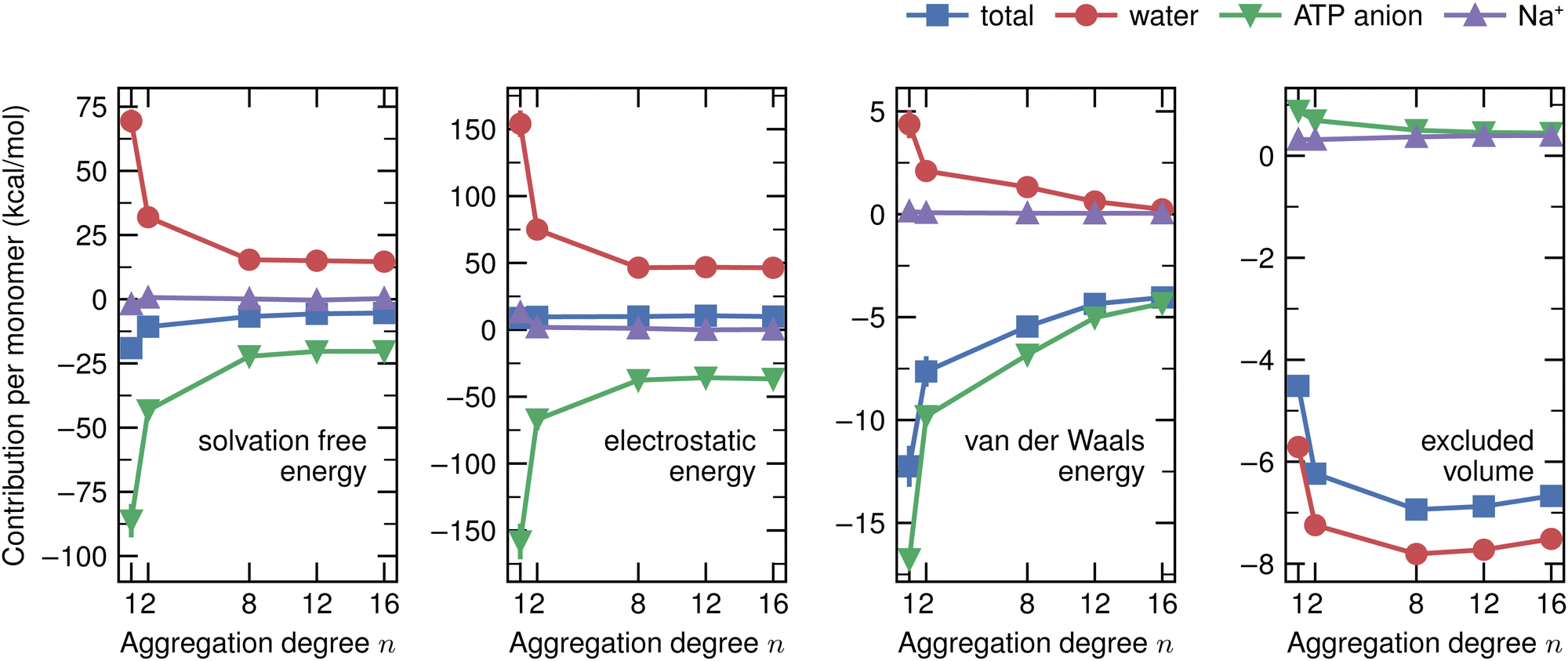
Fig. 3 shows the contributions of the electrostatic energy (blue lines, up-pointing triangles), van der Waals energy (green lines, down-pointing triangles), and excluded-volume effect (red lines, squares) with the (total) change of the solvation free energy (purple lines, circles). The magnitudes of the energy contributions in the water–ATP mixture are mostly larger compared to those in the water–urea system, although the concentration of ATP is 30 times lower. For example, the electrostatic contributions in the water–ATP mixture are more than twice the values in the water–urea mixture. The dependence of the electrostatic contribution on the degree of aggregation n is weak, though, with both ATP and urea. The electrostatic interaction is thus not decisive in determining the relative stabilities between the 1-mer and the aggregates. The excluded-volume effect favors the higher aggregation states with ATP while its n dependence is weak. The van der Waals interaction is the major contribution to the n dependence of the change of the solvation free energy with both cosolvents. In other words, while there are differences between the quantitative values of the energy components with ATP and urea as a cosolvent, the qualitative picture for the interaction governing the cosolvent effect is similar. This is an interesting result as the structures of those cosolvents are quite different in terms of size, charge, and flexibility. ATP may thus be viewed as a “big urea” in the sense that the van der Waals interaction leads to the peptide dissociation with minor roles played by the electrostatic components and that the aggregation is suppressed much more strongly with ATP. While it can be expected that the electrostatic contribution of urea is small compared to the van der Waals one,^{40,41,44–46} one might consider that the reverse is the case for ATP due to its high negative charge and because electrostatic interactions are stronger in general. In fact, several studies have pointed out that ATP adsorbs preferably onto the positively charged arginine and lysine residues of the peptides.^9,12–14,16 On the other hand, it has also been shown that triphosphate on its own cannot prevent the fibril formation of Aβ_1–42 while adenine and adenosine can, suggesting that the role of the phosphate group is to increase the solubility.¹¹ Our energy decomposition results are therefore in line with the experimental observations.

Fig. 3 Changes of the energy components per monomer upon ATP and urea addition. The electrostatic contribution is almost independent of n. The van der Waals interaction contributes the most to the stabilization of the 1-mer over the aggregates for both cosolvents. The changes of the solvation free energies are the same as in Fig. 2b. The error bar is expressed at 95% confidence interval (twice the standard error) and is not shown when the size of the data symbol is larger. Lines connecting the data points are drawn as guides for the eyes.

The energy components can be further decomposed into the contributions stemming from the cosolvent and water to gain deeper insights into the energetics:⁴⁰

The subscript i refers to the solvent species of our systems, i.e., water, ATP anion, Na⁺, or urea. Δu^elec_i and Δu^vdW_i are the electrostatic and van der Waals components with solvent species i, respectively. ε_i in the right-hand side of eqn (8) corresponds to the pair energy of the solute with solvent species i. By using eqn (6)–(8), we can define the solvation free energy contribution Δ〈ν^solv_i〉 of each solvent species i to the total change of the solvation free energy Δ〈ν^solv〉 asWith this definition, Δ〈ν^solv_i〉 is an additive quantity, i.e., it fulfills the following equation:

Hereafter, we use eqn (6)–(9) to obtain the contributions from each solvent species in the system with ATP as the cosolvent (Fig. 4): water (red lines, circles), ATP anion (green lines, down-pointing triangles), and Na⁺ (purple lines, up-pointing triangles). The contributions of Na⁺ to the dependencies of the changes of the solvation free energy and its components on the aggregation degree n are negligible and are therefore not discussed. The decomposition of the change of the solvation free energy reveals that the stabilization of the 1-mer over the aggregates after the introduction of ATP into the solvent environment stems almost solely from the ATP anion. Its contribution to Δ〈ν^solv〉 amounts to 65 kcal mol⁻¹ for the difference between the 1-mer and 16-mer, for example. This is partially compensated by water (−54 kcal mol⁻¹) and enhanced by Na⁺ (2 kcal mol⁻¹), resulting in the total Δ〈ν^solv〉 difference of 13 kcal mol⁻¹. The same trend can be observed for the decomposition of the van der Waals energy. The total van der Waals contribution amounts to 8 kcal mol⁻¹, which is due to the stabilizing effect of ATP (12 kcal mol⁻¹) with partial compensation by water (−4 kcal mol⁻¹). Regarding the electrostatic energy, there is a significant contribution stemming from the ATP anion which is an order-of-magnitude larger than the van der Waals one. This is in line with the expectation that the high charge of ATP should lead to strong electrostatic interactions. However, these are almost completely compensated by water, which explains our observation that the electrostatic interaction is almost independent of the aggregation degree n. The excluded-volume effect is almost solely due to water. Accordingly, water is in favor of the states with higher aggregation degrees for all of the electrostatic, van der Waals, and excluded-volume components while the ATP anion acts to suppress the aggregation.

Fig. 4 Decomposition of the changes of the energy components per monomer for each solvent species upon ATP addition. The largest contribution to the n dependence of the cosolvent-induced change of the total solvation free energy (blue lines, squares) stems from the ATP anion. ATP (green lines, down-pointing triangles) stabilizes the 1-mer whereas water (red lines, circles) favors higher aggregation degrees. The same trend is observed for the electrostatic and van der Waals energies. The n dependence of the excluded-volume effect stems almost solely from water. The contributions from Na⁺ can be neglected for all the cases. The total values are the same as in Fig. 3. The error bar is expressed at 95% confidence interval (twice the standard error) and is not shown when the size of the data symbol is larger. Lines connecting the data points are drawn as guides for the eyes.

We further decompose the electrostatic and van der Waals energies to analyze the contribution of each moiety within the ATP anion. The contributions of adenine (pink lines, circles), ribose (orange lines, down-pointing triangles), and phosphate (blue lines, up-pointing triangles) are shown in Fig. 5. Regarding the electrostatic energy, the contributions of adenine and ribose to the dependence on the aggregation degree n are small. The phosphate contribution almost matches the total ATP one. As for the van der Waals energy, all three moieties have a significant contribution. In particular for the difference between the 1-mer and the 16-mer, adenine has the largest contribution with ∼5.5 kcal mol⁻¹, followed by ribose and phosphate with ∼3.5 kcal mol⁻¹ each. It has been revealed by experiments¹¹ that adenine already can prevent the formation of amyloid fibrils. The fibrillation can be further suppressed when ribose is attached to adenine, and furthermore by phosphate. This series correlates with the finding in Fig. 5 that all three moieties contribute to the n dependence of the van der Waals component.

Fig. 5 Moiety contributions to the electrostatic and van der Waals energies between the ATP anion and the solutes. The electrostatic energy stems almost completely from phosphate. Adenine contributes the most to the van der Waals energy, followed by ribose and phosphate. The data for the total ATP anion is identical to the data in Fig. 4. The error bar is expressed at 95% confidence interval (twice the standard error) and is not shown when the size of the data symbol is larger. Lines connecting the data points are drawn as guides for the eyes.

Our last decomposition concerns the contributions of the sidechains and the backbones of the n-mers to the van der Waals energy. These are plotted in Fig. 6 for each moiety of ATP. The n dependence is larger for the sidechain with ∼7.5 kcal mol⁻¹ for the difference between the 1-mer and 16-mer. Within this difference, adenine has the largest contribution with ∼3.0 kcal mol⁻¹, while ribose and phosphate contribute with ∼2.0 kcal mol⁻¹ and ∼2.5 kcal mol⁻¹, respectively. The contribution of the backbone to the difference between the 1-mer and 16-mer amounts to roughly 5 kcal mol⁻¹, which is smaller than that of the sidechain but not negligible. It is composed of adenine with ∼2.5 kcal mol⁻¹, ribose with ∼1.5 kcal mol⁻¹, and phosphate with ∼1.0 kcal mol⁻¹.

Fig. 6 Contributions of the sidechain and backbone of the solute to the van der Waals energies with the ATP anion, as well as decompositions into the van der Waals energies with the moieties within ATP. The sidechain has a larger contribution compared to the backbone. More than half is from the adenine moiety. The ribose and phosphate moieties have similar contributions. The error bar is expressed at 95% confidence interval (twice the standard error) and is not shown when the size of the data symbol is larger. Lines connecting the data points are drawn as guides for the eyes.

We end our discussion by analyzing the structural features between ATP and the n-mers (Fig. 7) and connecting them with the energetic results. The spatial distribution function (SDF, Fig. 7a) reveals that ATP (gray) adsorbs onto the peptide surface. The SDF further shows that the ATP anion is accumulated primarily around the positively charged lysine residue and secondarily at hydrophobic sidechains like phenylalanine. While it can be observed that Na⁺ (purple) also adsorbs onto the peptide surface, especially around the oxygen atoms, Na⁺ is mostly gathered around the ATP anion. To quantify the adsorption, the number of contacts per solvent-accessible surface area (SASA) of the solute between each ATP moiety and the backbone and sidechain of the n-mers is plotted in Fig. 7b. The larger contribution stems from the sidechain (vibrant colors) while the backbone (faded colors) accounts for 10% to 30%. The total number of contacts per SASA is highest for the 1-mer and decreases with increasing aggregation degree. When the sidechain and backbone contributions are summed, adenine has the highest contribution, followed by ribose. The contribution of phosphate is smaller and corresponds to less than 50% of the one of adenine or ribose. We also determined the number of hydrogen bonds per SASA. Fig. 7b shows that the adenine and ribose moieties interact mainly with the backbone, contributing between 50% and 75%. The phosphate moiety, on the other hand, forms hydrogen bonds mainly with the sidechains while the backbone contributions are between 10% and 25%. The phosphate contributions are also larger than the ones of the adenine and ribose moieties combined. In accordance with the free-energy analysis, both plots in Fig. 7b reveal that the interaction with the 1-mer is the most favorable. It should be noted, though, that the relative importance of the interaction components can be addressed with the energetic analysis. While the adenine and ribose moieties make up for the most part of the number of contacts, the phosphate moiety forms most of the hydrogen bonds. It is therefore necessary to combine these results with the energetic analysis to get a picture of the mechanism behind the suppression of the fibrillation by ATP.

Fig. 7 Structural features between the solute and ATP. (a) Spatial distribution function (SDF) of the ATP anion (gray) and Na⁺ (purple) around a snapshot structure of the 1-mer. ATP (gray) adsorbs onto the peptide surface and is especially found around the positively charged lysine and the hydrophobic phenylalanine sidechains. Na⁺ (purple) is mainly gathered around ATP. The SDF of the ATP anion was determined by referring to all the atoms in ATP. The iso-density surfaces are drawn at the values equal to twice the bulk density. (b) Numbers of contacts and hydrogen bonds per SASA between the n-mers and ATP. The number of contacts (left) is dominated by the adenine and ribose moieties while the hydrogen bonds (right) are mainly formed by the phosphate moiety. Error bars equal twice the standard error (95% confidence interval).

A connection between the structural and energetic points of view can be made when the contributions of the ATP moieties in Fig. 7b are compared with the ones in Fig. 5. The electrostatic energy correlates with the number of hydrogen bonds as the phosphate moiety is dominant in both. Although the adenine and ribose moieties form hydrogen bonds with the solute, their contributions to the electrostatic energy are minor as the phosphate moiety involves high negative charges. Regarding the van der Waals energy, correlations with the number of contacts can be observed. For example, the phosphate moiety has the least and the adenine moiety the highest contribution. Although the ribose moiety has similar numbers of contacts as the adenine moiety, the latter exhibits stronger interactions like π-stacking with the sidechain of phenylalanine and has the more favorable (negative) van der Waals energy. With these connections, the suppression of the peptide fibrillation by ATP can be explained in the following way.

As discussed with Fig. 7, the ATP anion adsorbs onto the peptide surface through various types of non-covalent bonds. Fig. 7a shows that one major adsorption site is around the lysine residue. This is due to the hydrogen bonding between the negatively charged phosphate moiety and the positively charged lysine sidechain, which is the main contribution to the number of hydrogen bonds in Fig. 7b. From Fig. 7a, it is observed that ATP also adsorbs onto the aromatic sidechains of phenylalanine and the hydrophobic sidechains of valine and leucine. According to the number of contacts in Fig. 7b, this is mainly attributed to the adenine and ribose moieties. The underlying interactions can be the π-stacking between the adenine moiety and aromatic phenylalanine sidechains and the hydrophobic interactions of the adenine and ribose moieties with the hydrophobic sidechains. The comparison of Fig. 5 and 7b thus suggests that the hydrogen bonds correspond to electrostatic interactions, whereas the π-stacking and hydrophobic interactions are related to van der Waals interactions, in agreement with chemical intuition. As seen in Fig. 7b, the number of hydrogen bonds per SASA between ATP and the peptides is highest when the latter are not aggregated. This might lead to a view that the prevention of the fibrillation by ATP could be partially attributed to hydrogen bonds formed between ATP and the peptides. However, the resulting difference in the electrostatic energy between the aggregated and the monomeric state is small if the whole system is taken into account (Fig. 3). The energy decomposition in Fig. 4 reveals together with Fig. 5 that water cancels the electrostatic energy gain resulting from the higher number of hydrogen bonds per SASA formed by the phosphate moiety with the 1-mer. On the other hand, according to Fig. 4, the formation of π-stacking and hydrophobic interactions leads to the strongest gain of the van der Waals energy if the peptides are in the monomeric state. The van der Waals contribution dominates over the electrostatic one, which is in line with experimental observations that the amyloid fibrillation can be suppressed even when the phosphate moiety is removed from ATP.¹¹ Note that although the van der Waals interaction of the adenine moiety with the sidechains has the highest contribution (Fig. 6), it amounts only to 10% to 25% of the total van der Waals energy. Therefore, the suppression of the amyloid fibrillation by ATP cannot be attributed to a single type of interaction, but reflects the interactions of all three moieties of ATP with both the sidechain and backbone of the peptides.

Fig. 3 shows that the van der Waals component contributes the most to the solvation free energy change upon the introduction of ATP into the solution, leading to the free energy most favorable for the 1-mer. The equilibrium is then shifted from the fibril towards the 1-mer as illustrated in Fig. 2c and d. Note that for urea, the van der Waals interactions are also the main contribution to the stabilization of the 1-mer over the aggregate structures, whereas the electrostatic interactions have a minor effect.^{40,41,44–46} This shows that ATP and urea suppress the amyloid fibril formation through similar mechanisms from the viewpoint of energy decomposition.

4 Conclusions

The van der Waals interaction between ATP and the amyloid peptides was identified to be the driving force for the suppression of fibril formation upon the addition of ATP. It was also revealed that ATP is two orders of magnitude more effective than urea (when compared at the same molar concentrations) due to the ability of ATP to form stronger van der Waals interactions with peptides. This suggests that an effective way to destabilize amyloid fibrils is to strengthen the van der Waals interactions between the cosolvent and the solute. Note that our scheme is not limited to ATP and urea and can be used for any cosolvent, including those containing arginine and guanidium.^47–50 Accordingly, this work will help to design even more effective cosolvents to control the amyloid fibrillation and other aggregation processes.

Data availability

The molecular structure, topology, and parameter files required for the MD simulations and the free-energy analyses have been deposited at Zenodo (DOI: https://doi.org/10.5281/zenodo.8394729).

Author contributions

The study was conceived by T. M. D., D. H., and N. M. and supervised by D. H. and N. M. T. M. D. carried out the simulations and analysis. All authors discussed the results and contributed to the writing of the manuscript.

Conflicts of interest

The authors declare no competing interests.

Appendices

Appendix A: Detailed procedures of computation

The periodic boundary condition was employed with minimum image convention. The electrostatic interactions were computed using the smooth particle–mesh Ewald summation with a real-space cutoff of 1.4 nm, an interpolation order of 4, a relative tolerance of 10⁻⁵, and a Fourier spacing of 0.12 nm.⁵¹ The Lennard-Jones potential was truncated for distances greater than 1.4 nm and shifted such that it is zero at the cutoff. Long-range dispersion correction for energy and pressure as implemented in GROMACS was employed during the simulations for the Lennard-Jones potential. The Lennard-Jones parameters between unlike pairs of atoms were combined with the Lorentz–Berthelot combination rules. The LINear Constraint Solver (LINCS) algorithm was employed to fix the lengths of all bonds of Aβ_16–22, ATP, and urea.⁵² The water molecules were treated as rigid by using the SETTLE algorithm.⁵³ The leap-frog algorithm was adopted to integrate the equations of motion with a time step of 2 fs. The systems were coupled to a v-rescale thermostat with a coupling time of 0.1 ps to set the temperature to 300 K.⁵⁴

To prepare the initial configuration of the 2-mer, we placed two 1-mers laterally next to each other with a distance of 0.5 nm between their respective centers of geometry. The N-terminus of one peptide faced the C-terminus of the other with center-of-mass distances of roughly 0.7 nm between the α-carbons of the N- and C-termini, resulting in an antiparallel configuration. As for the 8-, 12-, and 16-mer aggregates, we started by first constructing the antiparallel β-sheets. For this, we placed six 1-mers side by side to form an antiparallel β-sheet with distances of 0.5 nm between the respective centers of geometry of the constituent monomers and of 0.7 nm between the N- and C-termini of the neighboring monomers as done for the 2-mer. The box dimension in the lateral direction was set to 2.88 nm so that the last monomer is placed next to the periodic image of the first one, which essentially results in an infinitely long β-sheet. An energy minimization with the steepest descent method with a maximum force threshold of 239 kcal mol⁻¹ nm⁻¹ (1000 kJ mol⁻¹ nm⁻¹) was carried out, followed by a simulation in vacuum for 250 ps. The four monomers in the middle were then extracted from the last configuration to form the antiparallel β-sheet of the aggregates. We stacked two, three, or four of these sheets on top of each other with a 1 nm spacing between the centers of geometry of the β-sheets. The sheets were stacked in parallel configuration, i.e., the C-termini of one sheet faced the C-termini of the other sheet with center-of-mass distances of roughly 1 nm between the α-carbons and likewise for the N-termini. The resulting structures were used as the starting configurations of the solutes.

The solute structure was sampled through the simulation in pure water with the solute left flexible, and when the energetics were analyzed, frozen structures of the solute were used. The simulations were carried out in the canonical (NVT) ensemble. For the pure-water solvent, the number of water molecules is 30 000. For the ATP–water mixture, 60 ATP anions and 240 Na⁺ counterions were used which corresponds to 100 mM of ATP. For the 3 M urea solution, we substituted 1770 water molecules with urea molecules as this number was also used in previous works.^40–42 The sum of all solvent molecules equals 30 000 for all studied systems. In order to determine the sizes of the simulation boxes, we additionally performed simulations without the solute in the isothermal–isobaric (NPT) ensemble for 1 ns. For these simulations, the pressure was set to 1 bar by coupling the system isotropically to the Parrinello–Rahman barostat at a coupling time of 1 ps and an isothermal compressibility of 4.5 × 10⁻⁵ bar⁻¹.⁵⁵ All other setup parameters were identical to those in NVT. The resulting box lengths in all three dimensions were 9.65 nm, 9.71 nm, and 9.93 nm for the pure-water system, ATP solution, and urea solution, respectively. For the NVT simulations of the system with solute, we used the same box size as the one without solute.

To sample the structure of the flexible solute, MD simulations were conducted in the pure-water solvent. First, the solute structure was energy-minimized in vacuum with the steepest descent method until the maximum force is smaller than 239 kcal mol⁻¹ nm⁻¹ (1000 kJ mol⁻¹ nm⁻¹). Then, 30 000 water molecules were inserted into the system. To equilibrate the water configuration, the solute was kept frozen and only the water molecules were energy-minimized, followed by a 1 ns simulation. After these equilibration steps, the flexible solute was simulated with water for 150 ns. To avoid possible loss of the β-sheet structure, we used flat-bottom potentials of the form

with a force constant k of 239 kcal mol⁻¹ nm⁻² (1000 kJ mol⁻¹ nm⁻²) and a threshold distance d of 0.7 nm. r is the distance between the α-carbon atoms and Θ refers to the Heaviside step function. This potential was employed only between the α-carbons of the terminal amino acid residues of adjacent peptides within the antiparallel β-sheets, i.e., between the lysine and the glutamate residues. No restraints were employed between the residues of parallel β-sheets.

The number of contacts was determined with the “gmx mindist” tool of GROMACS.³⁶ The solute was considered to be in contact with an ATP anion when the atom–atom distance for any pairs of atoms from the solute and ATP is less than 0.6 nm. The solvent-accessible surface areas (SASAs) were further obtained with the “gmx sasa” tool of GROMACS.^36,56 For each n-mer, we computed the SASAs of the backbone and the sidechain for each of the 50 fixed configurations and used their average values. The number of hydrogen bonds were calculated using the “gmx hbond” tool of GROMACS.³⁶ A hydrogen bond is present between a donor and an acceptor when the donor–acceptor distance is equal or smaller than 0.35 nm and the hydrogen-donor–acceptor angle is equal or smaller than 30°.

Fig. 8 shows the SASA per monomer of the flexible solute during the simulation in pure water with a sampling interval of 100 ps. It can be observed that the SASAs of the 1- and 2-mers vary significantly over time. This behaviour is expected as these two structures are relatively flexible, allowing several conformational changes during the simulation. In contrast, the SASAs of the 8-, 12-, and 16-mers fluctuate stably around an average value due to the (relative) rigidity of the aggregates. Further, the SASA per monomer decreases with increasing aggregation degree n, as additional monomers are burried inside the aggregate, making them less exposed to the solvent. This effect is stronger when transitioning from the 8- to the 12-mer compared to going from the 12- to the 16-mer, as the contribution of the constituents on the surface becomes less relevant.

Fig. 8 Solvent-accessible surface areas (SASAs) per monomer of the n-mers. The SASA per monomer of the 1-mer (monomer), 2-mer (dimer), 8-mer, 12-mer, and 16-mer are shown. The average value of the SASA per monomer is 13.28, 9.80, 5.87, 4.91, and 4.79 nm², respectively, with a standard deviation of 0.57, 0.61, 0.16, 0.15, and 0.11 nm².

We computed the solvation free energies for all the solute structures in the pure-water solvent, the ATP–water mixed solvent, and the urea–water mixed solvent using the method of energy representation.²⁷ In this method, an approximate functional is used to determine the free energy from a set of energy distribution functions which are obtained from a simulation of the solution system of interest and from a simulation of a reference system. In the solution system of interest, the position and orientation of the solute was kept fixed. The distribution function was computed for the pair-interaction energy between the solute and the solvent. The solute was the Aβ_16–22 peptide, its 2-mer, 8-mer, 12-mer, or 16-mer. For the reference system, a simulation was performed without the solute and a test-particle insertion of the solute into the solvent system was implemented. The density of states for the solute–solvent pair potential and the solvent–solvent pair correlation were calculated against the solute molecule which was virtually present in the system and did not influence the solvent configuration. The approximate functional used to obtain the solvation free energy is given in ref. 27. The self-energy term as given in ref. 27 was not incorporated into the value of the solvation free energy in this work as it is negligible (∼0.1 kcal mol⁻¹).

The procedures for simulating the solution systems of interest are as follows. In the case of the pure-water solvent, the solute–water configuration from the simulation with the flexible solute in water was used without modification as the starting configuration for the simulation of the solution system. For the ATP–water and urea–water mixtures as the (mixed) solvents, the solute structure extracted from the solute–water configuration was first solvated by the mixed solvent and was then energy-minimized only for the solvent molecules with the steepest descent method until the maximum force was smaller than 239 kcal mol⁻¹ nm⁻¹ (1000 kJ mol⁻¹ nm⁻¹). The run lengths of equilibration and production and the sampling intervals for the solution systems of interest are listed in Table 1. When the solvent was of water, ATP, and Na⁺, 5 simulations were performed with different solvent configurations per frozen solute structure. We therefore conducted a total of 250 simulations per solute in the ATP–water mixed solvent.

To carry out the simulations of the reference system for the pure-water solvent, an equilibration run of 1 ns and a production run of 5 ns were conducted with a sampling interval of 1 ps. To simulate the ATP–water mixture, the reference solvent was equilibrated for 50 ns and a production run was done for 50 ns with a sampling interval of 0.5 ps. For the urea–water mixture, the equilibration time was 5 ns, the production run time was 20 ns, and the sampling interval was 1 ps. The internal coordinates of the solute were identical between the solution system and the corresponding reference system where the solute was inserted as a test particle. The test-particle insertion of the solute was performed 200 times per reference-solvent configuration frame at random positions. The orientation of the solute at the insertion in the reference system was set identical to the one in the solution system to exclude possible variation of the self energy due to the orientation of the solute which would otherwise occur as a finite-size effect.

The errors for the energy values were estimated through the procedure in Appendix B of Masutani et al.⁴⁰ It should be noted that the 95% confidence interval is provided by multiplying a factor of 2 to eqn (B4) of Masutani et al.⁴⁰

Appendix B: Derivation of eqn (3)

The equilibrium between the monomeric and aggregate states will be shifted upon addition of a cosolvent due to the changes of the intermolecular interactions of the solutes and the corresponding changes of the excess chemical potentials. To examine how μ^ex_n of aggregation state n as given by eqn (2) varies when a cosolvent of concentration c is added at constant temperature, the following expression is useful:^40,41This is an exact expression, and for its derivation, we have supposed that for unpolarizable forcefields, the intra-solute energy E_S(ψ_n) for a fixed structure ψ_n is independent of the solvent environment. Eqn (A2) shows in particular that it is not necessary to compute the configurational entropy term. This is a useful result as the computation of the configurational entropy still poses a challenge and is under active development.^57–60 According to eqn (A2), it is sufficient to determine the change of the solvation free energy over a set of fixed structures of the solute and average them to obtain the change of the excess chemical potential due to the cosolvent addition.

When we expand the excess chemical potential μ^ex_n and the solvation free energy ν^solv(ψ_n) as Taylor series around c = 0 (pure-water solvent),

eqn (3) follows through eqn (A2)–(A4). This justifies our approach to use the set of solute structures obtained from the simulation in the pure-water solvent to determine the cosolvent-induced change of the excess chemical potential.

Appendix C: Dependence of the solvation free energy change on the cosolvent concentration

To investigate the dependence of Δ〈ν^solv〉/n on the cosolvent concentration, we carried out additional simulations for the 1-mer and 16-mer with 50 and 75 mM ATP, which correspond to 30 and 45 ATP anions in the MD unit cell, respectively. For urea, the concentrations of the additional simulations were 1 and 2 M, which contain 590 and 1180 urea molecules, respectively. The box dimensions were determined according to the procedure described in the third paragraph in Appendix A. For the systems with the 1-mer and ATP as the cosolvent, all of the 50 configurations used to compute Δ〈ν^solv〉/n at 100 mM were also employed at 50 and 75 mM, and the simulations of the solution systems of interest were performed 5 times per solute configuration as done at 100 mM. For the 16-mer with 50 and 75 mM ATP and the 1- and 16-mers with 1 and 2 M urea, 5 configurations were taken from the MD of the flexible solute in pure water at 60, 80, 100, 120, and 140 ns and the solvation free energies were computed by running the simulations of the solution systems once per solute configuration. The solvation free energies were computed according to the scheme noted in Appendix A. Fig. 9 displays the cosolvent-induced changes of the averaged solvation free energy per monomer Δ〈ν^solv〉/n upon addition of ATP (left) and urea (right). The lines are least-square fits with the intercept kept fixed at 0. For the ATP cosolvent, the values for the 16-mer lie on the fit, whereas deviations from the fit can be observed for the 1-mer. When the value at 50 mM is adopted, the suppression factor Sp increases by 40% to 50% from the one obtained with the 100 mM data and provided in Fig. 2d. Still, the discussion in the main text is valid and the conclusions are not altered. For the urea cosolvent, Δ〈ν^solv〉/n changes linearly with the cosolvent concentration.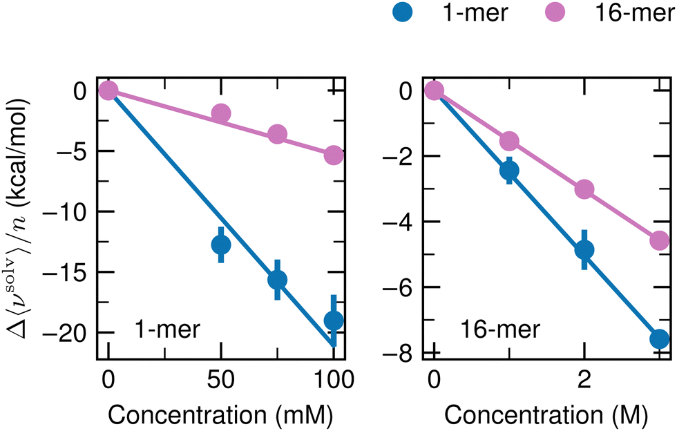

Fig. 9 Dependency of Δ〈ν^solv〉/n on the cosolvent concentration. Δ〈ν^solv〉/n was determined for the 1-mer (blue) and 16-mer (pink) at ATP concentrations of 50, 75, and 100 mM (left) and at 1, 2, and 3 M with urea (right). Δ〈ν^solv〉/n at 100 mM with ATP and at 3 M with urea are the same as in Fig. 2b. The error bar is expressed at 95% confidence interval (twice the standard error) and is not shown when the size of the data symbol is larger. The straight lines are the least-square fits with zero intercepts over the three concentrations of the cosolvents.

Acknowledgements

The authors thank Stefan Hervø-Hansen and Kento Kasahara of Osaka University for valuable discussion. This work is supported by the Grants-in-Aid for Scientific Research (No. JP22KF0240 and JP23H02622) from the Japan Society for the Promotion of Science, by the Fugaku Supercomputer Project (No. JPMXP1020230325 and JPMXP1020230327) and the Data-Driven Material Research Project (No. JPMXP1122714694) from the Ministry of Education, Culture, Sports, Science, and Technology, and by Maruho Collaborative Project for Theoretical Pharmaceutics. The simulations were conducted partly using Cygnus at Tsukuba University, Flow at Nagoya University, Ito at Kyushu University, and Fugaku at RIKEN Advanced Institute for Computational Science through the HPCI System Research Project (Project IDs: hp230101, hp230205, and hp230212). T. M. D. is grateful to the Postdoctoral Fellowship for Research in Japan (No. PE21718) from the Japan Society for the Promotion of Science.

Notes and references

1. A. Patel, L. Malinovska, S. Saha, J. Wang, S. Alberti, Y. Krishnan and A. A. Hyman, Science, 2017, 356, 753–756.
2. F. Chiti and C. M. Dobson, Annu. Rev. Biochem., 2006, 75, 333–366.
3. S. Jarvis and A. Mostaert, The Functional Fold: Amyloid Structures in Nature, CRC Press, 2012.
4. D. E. Otzen, Amyloid Fibrils and Prefibrillar Aggregates: Molecular and Biological Properties, John Wiley & Sons, 2013.
5. Y. E. Kim, M. S. Hipp, A. Bracher, M. Hayer-Hartl and F. Ulrich Hartl, Annu. Rev. Biochem., 2013, 82, 323–355.
6. J. Labbadia and R. I. Morimoto, Annu. Rev. Biochem., 2015, 84, 435–464.
7. J. Kang, L. Lim, Y. Lu and J. Song, PLoS Biol., 2019, 17, e3000327.
8. J. Kang, L. Lim and J. Song, Commun. Biol., 2019, 2, 1–10.
9. S. Pal and S. Paul, J. Phys. Chem. B, 2020, 124, 210–223.
10. R. Roy and S. Paul, J. Phys. Chem. B, 2021, 125, 3510–3526.
11. J. Mehringer, T.-M. Do, D. Touraud, M. Hohenschutz, A. Khoshsima, D. Horinek and W. Kunz, Cell Rep. Phys. Sci., 2021, 2, 100343.
12. M. Nishizawa, E. Walinda, D. Morimoto, B. Kohn, U. Scheler, M. Shirakawa and K. Sugase, J. Am. Chem. Soc., 2021, 143, 11982–11993.
13. J. Song, Protein Sci., 2021, 30, 1277–1293.
14. G. Hu, X. Ou and J. Li, J. Phys. Chem. B, 2022, 126, 4647–4658.
15. H. Aida, Y. Shigeta and R. Harada, Proteins: Struct., Funct., Bioinf., 2022, 90, 1606–1612.
16. M. Zalar, J. Bye and R. Curtis, J. Am. Chem. Soc., 2023, 145, 929–943.
17. T. Mori and N. Yoshida, J. Chem. Phys., 2023, 159, 035102.
18. S. Lenton, S. Hervø-Hansen, A. M. Popov, M. D. Tully, M. Lund and M. Skepö, Biomacromolecules, 2021, 22, 1532–1544.
19. J. Bye, K. Murray and R. Curtis, Biomedicines, 2021, 9, 1646.
20. M. Calamai, J. R. Kumita, J. Mifsud, C. Parrini, M. Ramazzotti, G. Ramponi, N. Taddei, F. Chiti and C. M. Dobson, Biochemistry, 2006, 45, 12806–12815.
21. K. Yamaguchi, M. So, C. Aguirre, K. Ikenaka, H. Mochizuki, Y. Kawata and Y. Goto, J. Biol. Chem., 2021, 296, 100510.
22. A. Hautke and S. Ebbinghaus, Biol. Chem., 2023, 404, 897–908.
23. N. Matubayasi and M. Nakahara, J. Chem. Phys., 2000, 113, 6070–6081.
24. N. Matubayasi and M. Nakahara, J. Chem. Phys., 2002, 117, 3605–3616.
25. N. Matubayasi and M. Nakahara, J. Chem. Phys., 2003, 118, 2446.
26. N. Matubayasi and M. Nakahara, J. Chem. Phys., 2003, 119, 9686–9702.
27. S. Sakuraba and N. Matubayasi, J. Comput. Chem., 2014, 35, 1592–1608.
28. F. Timur Senguen, N. R. Lee, X. Gu, D. M. Ryan, T. M. Doran, E. A. Anderson and B. L. Nilsson, Mol. BioSyst., 2011, 7, 486–496.
29. S. A. Petty and S. M. Decatur, J. Am. Chem. Soc., 2005, 127, 13488–13489.
30. J. J. Balbach, Y. Ishii, O. N. Antzutkin, R. D. Leapman, N. W. Rizzo, F. Dyda, J. Reed and R. Tycko, Biochemistry, 2000, 39, 13748–13759.
31. Y. Wang, S. J. Bunce, S. E. Radford, A. J. Wilson, S. Auer and C. K. Hall, Proc. Natl. Acad. Sci. U. S. A., 2019, 116, 2091–2096.
32. S. T. Ngo, X.-C. Luu, N. T. Nguyen, V. V. Vu and H. T. T. Phung, PLoS One, 2018, 13, e0204026.
33. S. Gnanakaran, R. Nussinov and A. E. García, J. Am. Chem. Soc., 2006, 128, 2158–2159.
34. S. G. Itoh and H. Okumura, Int. J. Mol. Sci., 2021, 22, 1859.
35. D. A. Case, I. Y. Ben-Shalom, S. R. Brozell, D. S. Cerutti, T. E. Cheatham, III, V. W. D. Cruzeiro, T. A. Darden, R. E. Duke, D. Ghoreishi, M. K. Gilson, H. Gohlke, A. W. Goetz, D. Greene, R. Harris, N. Homeyer, Y. Huang, S. Izadi, A. Kovalenko, T. Kurtzman, T. S. Lee, S. LeGrand, P. Li, C. Lin, J. Liu, T. Luchko, R. Luo, D. J. Mermelstein, K. M. Merz, Y. Miao, G. Monard, C. Nguyen, H. Nguyen, I. Omelyan, A. Onufriev, F. Pan, R. Qi, D. R. Roe, A. Roitberg, C. Sagui, S. Schott-Verdugo, J. Shen, C. L. Simmerling, J. Smith, R. Salomon-Ferrer, J. Swails, R. C. Walker, J. Wang, H. Wei, R. M. Wolf, X. Wu, L. Xiao, D. M. York and P. A. Kollman, AMBER 2018, 2018.
36. M. J. Abraham, T. Murtola, R. Schulz, S. Páll, J. C. Smith, B. Hess and E. Lindahl, SoftwareX, 2015, 1–2, 19–25.
37. J. L. F. Abascal and C. Vega, J. Chem. Phys., 2005, 123, 234505.
38. R. B. Best and J. Mittal, J. Phys. Chem. B, 2010, 114, 8790–8798.
39. C. Hölzl, P. Kibies, S. Imoto, J. Noetzel, M. Knierbein, P. Salmen, M. Paulus, J. Nase, C. Held, G. Sadowski, D. Marx, S. M. Kast and D. Horinek, Biophys. Chem., 2019, 254, 106260.
40. K. Masutani, Y. Yamamori, K. Kim and N. Matubayasi, J. Chem. Phys., 2019, 150, 145101.
41. N. Matubayasi and K. Masutani, Biophys. Physicobiol., 2019, 16, 185–195.
42. N. Matubayasi, Chem. Commun., 2021, 57, 9968–9978.
43. J. R. Kim, A. Muresan, K. Y. C. Lee and R. M. Murphy, Protein Sci., 2004, 13, 2888–2898.
44. M. Lindgren and P.-O. Westlund, Phys. Chem. Chem. Phys., 2010, 12, 9358–9366.
45. C. Y. Hu, H. Kokubo, G. C. Lynch, D. W. Bolen and B. M. Pettitt, Protein Sci., 2010, 19, 1011–1022.
46. Y. Yamamori, R. Ishizuka, Y. Karino, S. Sakuraba and N. Matubayasi, J. Chem. Phys., 2016, 144, 085102.
47. D. Shukla and B. L. Trout, J. Phys. Chem. B, 2010, 114, 13426–13438.
48. T. Kawasaki and S. Kamijo, Biosci., Biotechnol., Biochem., 2012, 76, 762–766.
49. F. Saczewski and Ł. Balewski, Expert Opin. Ther. Pat., 2009, 19, 1417–1448.
50. P. Gehlot, S. Kumar, V. Kumar Vyas, B. Singh Choudhary, M. Sharma and R. Malik, Bioorg. Med. Chem., 2022, 74, 117047.
51. U. Essmann, L. Perera, M. L. Berkowitz, T. Darden, H. Lee and L. G. Pedersen, J. Chem. Phys., 1995, 103, 8577–8593.
52. B. Hess, H. Bekker, H. J. C. Berendsen and J. G. E. M. Fraaije, J. Comput. Chem., 1997, 18, 1463–1472.
53. S. Miyamoto and P. A. Kollman, J. Comput. Chem., 1992, 13, 952–962.
54. G. Bussi, D. Donadio and M. Parrinello, J. Chem. Phys., 2007, 126, 014101.
55. M. Parrinello and A. Rahman, J. Appl. Phys., 1981, 52, 7182–7190.
56. F. Eisenhaber, P. Lijnzaad, P. Argos, C. Sander and M. Scharf, J. Comput. Chem., 1995, 16, 273–284.
57. M. Karplus and J. N. Kushick, Macromolecules, 1981, 14, 325–332.
58. U. Hensen, O. F. Lange and H. Grubmüller, PLoS One, 2010, 5, e9179.
59. K. W. Harpole and K. A. Sharp, J. Phys. Chem. B, 2011, 115, 9461–9472.
60. S. Hikiri, T. Yoshidome and M. Ikeguchi, J. Chem. Theory Comput., 2016, 12, 5990–6000.

---