What governs magnetic exchange couplings in radical-bridged dinuclear complexes?†
Received
22nd December 2023
, Accepted 1st February 2024
First published on 7th February 2024
Abstract
Coupling transition metal or lanthanide ions through a radical bridging ligand is a promising route to increase performances in the area of single molecular magnets. A better understanding of the underlying physical mechanisms governing the magnetic exchange couplings is thus of valuable importance to design future compounds. Here, couplings in three series of metal–radical–metal compounds based on transition metal ions are investigated by means of the decomposition/recomposition methods. This work presents the generalisation and first application of the method to systems with an arbitrary number of magnetic centres featuring several unpaired electrons. Thanks to the decomposition into the three main contributions (direct exchange, kinetic exchange, and spin polarisation) as well as a description in terms of electron–electron interactions, we study the influence of the nature of the metal centre and the radical ligand on the couplings. We combine the energetic contributions extracted with orbital and charge population analysis to rationalise the results.
Single-molecule magnets (SMM) are molecules capable of retaining magnetisation under a certain temperature, so-called blocking temperature. In the search for compounds with high blocking temperatures, complexes with radical bridging transition metal- or lanthanide-based paramagnetic centres have emerged as one of the most promising families of molecules.1–7 Indeed, the couplings occurring between each ion centre and the radical yield a strong indirect ferromagnetic coupling which may increase this property.8,9 Understanding the physical mechanisms governing these couplings is thus of great interest in guiding the design of future compounds.
Theoretical and computational chemistry, where the magnetic exchange coupling J is computed as the energy difference between the spin states, has played a critical role in providing molecular magnetism with both conceptual tools and numerical analysis.10 Wave-function-based methods have been specially well suited for this dual purpose where the dynamic correlation is usually accounted on top of a CASSCF wave-function,11 through mostly CI12 or PT2 treatment.13–18 This strategy provides highly accurate results where the proper physical description of the multiconfigurational character of the spin states is essential. In addition, the resulting wave-functions are dense objects from which much information may be extracted with the combination of model Hamiltonians and the effective Hamiltonian theory, providing a deep rationalisation of the physical mechanisms of magnetic phenomena.10,19–23 However, this sophistication results in a computational cost which is most of the time prohibitive for real-life applications.
To overcome this limitation, density functional theory (DFT) in its Kohn–Sham formulation24,25 has been the most used alternative with the first calculations of magnetic exchange couplings in the early 80's.26,27 However, this strategy is not exempt from its own drawbacks since (i) KS-DFT is intrinsically a monodeterminantal theory and the computation of J resorts to the use of Broken–Symmetry (BS) configurations,26–35 (ii) there is a strong dependence on the exchange–correlation functional which has been widely studied over the last two decades22,36–42 and (iii) the fact that this approach provides an energy difference only but no information about the underlying physical mechanisms.
Ferré et al. have provided a solution to this last limitation with the decomposition method, which allows decomposing the magnetic exchange coupling computed in DFT in its 3 main physical contributions: the ferromagnetic direct exchange J0 between the magnetic centres, the antiferromagnetic kinetic exchange ΔJKE resulting from the relaxation of the magnetic orbitals and the spin polarisation ΔJSP due to the different field felt by the non-magnetic electrons in the different states. This decomposition based on the Heinsenberg–Dirac–van Vleck (HDvV) Hamiltonian has been successfully applied in various situations with two unpaired electrons such as dinuclear complexes,43 quantum spin liquids44 or radical systems.45 Recently, the present authors have shown the relevance of the method in dinuclear complexes with more than one unpaired electron per magnetic centre.46 In addition, this method has been generalised to systems with an arbitrary number of one-unpaired-electron-based magnetic sites by employing the more general Hubbard Hamiltonian.47–49 This strategy provides a solution to the long-standing question of the spin contamination of J couplings in multicentre systems by summing up these three properly spin-decontaminated contributions.49
This work presents the complete generalisation of this newly developed decomposition/recomposition method to polynuclear magnetic systems featuring several unpaired electrons per magnetic centre. This method is applied to metal–radical–metal complexes to investigate both the influence of the metal centre and the role of the bridging ligand on the magnetic exchange couplings. This paper is organised as follows. Section 1 presents the computation of the different contributions to the magnetic exchange couplings in multicentre systems with a special focus on the t and U Hubbard Hamiltonian parameters in the context of several unpaired electrons. In Section 2, we present the three series of compounds studied in this work, i.e. the M–tetraazalene–M (with M = Cr, Mn, Fe and Co) series,50 the M–semiquinone–M (with M = Fe, Co and Ni) series51 and a series based on bis(bidentate) benzosemiquinoid-based radical bridging two Cr ions.52 Details of calculations are provided in Section 3. Section 4 discusses the decomposition in the three series, corroborated with orbital and charge population analysis. Finally, an open-source input files generator code that we have developed to ease the use of the method is shortly introduced in Section S1 of the ESI.†
1 Methodology
Magnetic exchange couplings are mostly described through the HDvV Hamiltonian,| |  | (1) |
where JIJ expresses the strength of the coupling between two local high-spin sites I and J and  and
and  their local spin operators, respectively. Based on the pioneering work of De Loth et al.53 and later Calzado et al.19–21 in wave-function theory, Ferré et al.54,55 and recently in a more general form David et al.47–49 decomposed in KS-DFT the magnetic exchange coupling as,
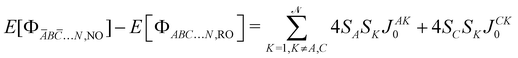
| | | JIJ = JIJ0 + ΔJIJKE + ΔJIJSP | (2) |
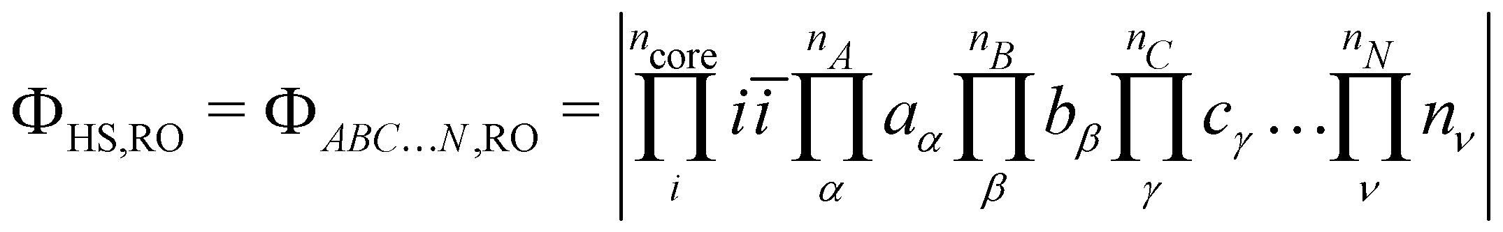
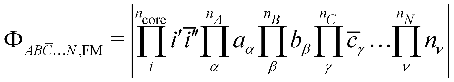
The following discussion presents the extraction of these three contributions and uses the notation introduced in ref. 49, of which the reader may refer to for further details. Let us consider a system with  magnetically coupled local high-spin sites labelled A, B, C, …, N, bearing nA, nB, nC, …, nN unpaired electrons, respectively, resulting in a maximum of
  couplings. To each magnetic centre is associated magnetic orbitals labelled with their lowercase letter aα, bβ, … and whose Greek letters are used for the summation over the number of unpaired electrons. Finally, i and j correspond to core orbitals, i.e. non-magnetic occupied ones, and r and s to virtual orbitals.
1.1 Direct exchange
The starting point of the method is the computation of the high-spin (HS) state in the restricted open-shell (RO) or in the quasi-restricted open-shell (QRO) formalism.56 This determinant of a (nA + nB + nC + … + nN + 1) spin multiplicity defines a set of ncore doubly occupied core orbitals i and a set of nA + nB + nC + … + nN singly occupied molecular orbitals (SOMOs), of which their localisation yields,| | 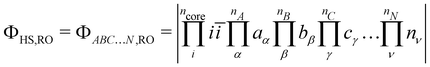 | (3) |
To determine the  direct exchange contributions,
  energy differences between the HS and some BS determinants must be defined. One may start by considering the
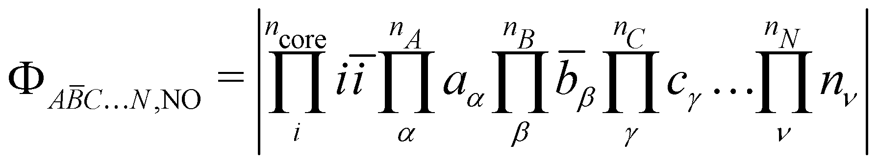
  configurations whose all spins of a magnetic site are flipped from the HS,RO determinant without optimising any orbital such as,
| | 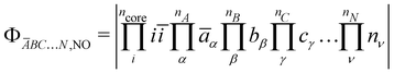 | (4) |
| |  | (5) |
| |  | (6) |
where NO stands for non-optimised. This leads to the following energy differences,| |  | (7) |
| |  | (8) |
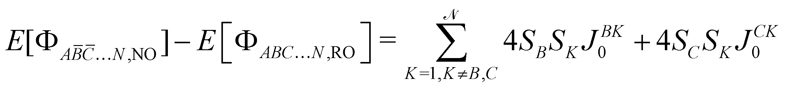
| |  | (9) |
with SA, SB,… the spin of the magnetic site A, B, …, respectively. The left  energy differences may be defined through the BS determinants with two magnetic sites flipped as,
| |  | (10) |
| |  | (11) |
| |  | (12) |
yielding,| | 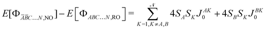 | (13) |
| |  | (14) |
| |  | (15) |
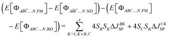
The  direct exchange contributions may be extracted from these two sets of energy differences by solving the set of linear equations.
1.2 Spin polarisation contribution
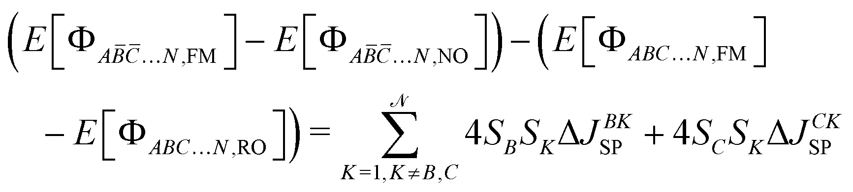
The spin polarisation contribution corresponds to the different responses felt by the core orbitals due to the different fields created by the magnetic electrons in the high and low spin states. Its extraction proceeds through the relaxation of the core orbitals in the previously generated HS,(Q)RO and BS,NO determinants and results in a substantially similar set of equations to solve as for the direct exchange. For the sake of conciseness, only the main working equations are presented and the reader should refer to ref. 49 for further discussions. Starting from the HS,RO determinant, the relaxation of the core orbitals is allowed while the magnetic orbitals are kept frozen,| |  | (16) |
where FM stands for frozen magnetic orbitals and the prime for the relaxed orbitals. Relaxing the core orbitals of the BS determinants with one magnetic centre flipped,| |  | (17) |
| |  | (18) |
| |  | (19) |
and of those with the spin of two magnetic centres flipped,| |  | (20) |
| |  | (21) |
| |  | (22) |
result in a set of  energy differences from which the direct exchange is retrieved,
| |  | (23) |
| |  | (24) |
| |  | (25) |
| |  | (26) |
| |  | (27) |
| |  | (28) |
1.3 Kinetic exchange
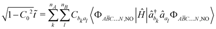
The kinetic exchange contribution is the main contribution to spin-decontaminate and this aspect is particularly challenging in systems involving several couplings since the Yamaguchi formula is no longer valid, whilst Shoji et al. provided an extension to multicentre systems based on spin correlation functions.49,57 To overcome the use of a spin-decontamination formula, some of the present authors proposed to proceed through the extraction of the t and U Hubbard parameters associated with one pair of magnetic centres.49 Considering a pair of magnetic centres A and B, this is done by relaxing A to B, and independently B to A. It results in two sets of t and U, which are equal in highly symmetric situations.
Let us consider the extraction of the Hubbard Hamiltonian parameters to determine the kinetic exchange contribution to the JAB coupling. Four relaxations may be considered (i) the occupied magnetic orbitals of A to the virtual magnetic orbitals B in the A![[B with combining macron]](https://www.rsc.org/images/entities/i_char_0042_0304.gif) …N situation, (ii) the same relaxation in the ĀB…N situation, (iii) the occupied magnetic orbitals of B to the virtual magnetic orbitals of A in the A…N situation and (iv) the same relaxation in the ĀB…N situation. As discussed in ref. 49, (i) and (ii) provide similar t and U parameters while the same is true for (iii) and (iv).
…N situation, (ii) the same relaxation in the ĀB…N situation, (iii) the occupied magnetic orbitals of B to the virtual magnetic orbitals of A in the A…N situation and (iv) the same relaxation in the ĀB…N situation. As discussed in ref. 49, (i) and (ii) provide similar t and U parameters while the same is true for (iii) and (iv).
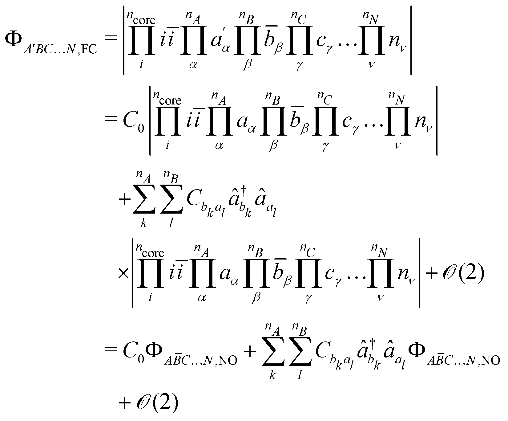
Let us now focus only on one of these extractions with the first relaxation to present the procedure in the context of several unpaired electrons per magnetic centre. This relaxation results in a reorganisation of the electronic distribution which may be thought of as slightly emptying the orbitals of A to fill the virtual orbitals of B,
| |  | (29) |
where
C0 and
Cbkal correspond to the normalized coefficients with

and

to some higher-order expansion determinants. The entry of these ionic-like forms in the wavefunction results in two sets of energetic contributions,
| |  | (30) |
The second term of the right-hand equation is homogeneous with the
U on-site repulsion energy Hubbard parameter while the last is homogeneous with the hopping integral
t. These terms correspond to some individual contributions from all
A orbital–
B orbital pairs. To avoid a laborious extraction of all these terms, let us define some overall effective
![[t with combining tilde]](https://www.rsc.org/images/entities/i_char_0074_0303.gif)
and
Ũ parameters capturing the relevant physics of the relaxation mechanism of the effective spin centre
A over
B as,
| |  | (31) |
with,
| |  | (32) |
| |  | (33) |
Hence, it results in a similar set of equations as for the one electron per centre case where both terms may be extracted by,
| |  | (34) |
| |  | (35) |
where,
| |  | (36) |
Pointing out that

,
α may be written in a simpler form as,
| |  | (37) |
Finally, the kinetic exchange contribution can be obtained by summing the Hubbard parameters resulting from both relaxations as,
| |  | (38) |
2 Molecular systems
To investigate both roles of the bridging ligand and of the metal centre in M–radical–M complexes, three series of compounds have been studied. The first series consists of 4 complexes presented in Fig. 1(a), [(TPyA)2CrIII2(NMePhL3−˙)]3+ and [(TPyA)2MII2(NMePhL3−˙)]+ (with M = MnII, FeII and CoII), where NMePhLH2 = N,N,N,N-tetra(2-methylphenyl)-2,5-diamino-1,4-diiminobenzoquinone; TPyA = tris(2-pyridyl-methyl)amine, labelled 1a, 2a, 3a and 4a, respectively.50 The couplings between the radical moiety and the metal centres have been experimentally determined by fitting the χT versus T magnetic susceptibility curve using the following HDvV model Hamiltonian,| | 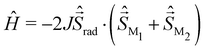 | (39) |
These complexes present large antiferromagnetic couplings ranging from −157 cm−1 for 2a to −626 cm−1 for 1a and are detailed in Table 1. This series of tetraazalene radical-based compounds has been previously studied by Singh using DFT calculations.58
 |
| | Fig. 1 Schematic representations of (a) the tetraazulene-based series M = CrIII, MnII, FeII and CoII, (b) the semiquinone-based series with M = FeII, CoII and NiII, (c) the benzosemiquinoid-based series with M = CrIII, and (d) atom numbering of the benzosemiquinoid-based series of Table 8. | |
Table 1 Formula, electronic configuration of the M centre and experimental magnetic exchange coupling in cm−1 of the M–radical–M complexes
|
|
Complex |
M |
Configuration |
J
M–Radexp
|
|
1a
|
[(TPyA)2CrIII2(NMePhL3−˙)]3+ |
CrIII |
d3 |
−626 |
|
2a
|
[(TPyA)2MnII(NMePhL3−˙)]+ |
MnII |
d5 |
−157 |
|
3a
|
[(TPyA)2FeII(NMePhL3−˙)]+ |
FeII |
d6 |
−307 |
|
4a
|
[(TPyA)2CoII(NMePhL3−˙)]+ |
CoII |
d7 |
−396 |
|
3b
|
[(Me6tren)2FeII2(C6H4O22−˙)]3+ |
FeII |
d6 |
−144 |
|
4b
|
[(Me6tren)2CoII2(C6H4O22−˙)] |
CoII |
d7 |
−252 |
|
5b
|
[(Me6tren)2NiII2(C6H4O22−˙)]3+ |
NiII |
d8 |
<−600 |
|
1cO
|
[(TPyA)2CrIII2(OL3−˙)]3+ |
CrIII |
d3 |
−352 |
|
1cOS
|
[(TPyA)2CrIII2(OSL3−˙)]3+ |
CrIII |
d3 |
−401 |
|
1cS
|
[(TPyA)2CrIII2(SL3−˙]3+ |
CrIII |
d3 |
−487 |
The second series (Fig. 1(b)) is based on semiquinone radical with a [(Me6tren)2MII2(C6H4O22−˙)]3+ architecture with Me6tren = tris(2-dimethylaminoethyl)amine and M = Fe, Co, Ni, labelled 3b, 4b and 5b, respectively.51 Here again, radical–metal couplings have been determined by fitting the same model Hamiltonian over χT versus T curve, resulting in strong antiferromagnetic couplings presented in Table 1.
Finally, a third series of three complexes consisting in CrIII ions linked through a bis(bidentate) benzosemiquinoid-based radical, [(TPyA)2Cr2(RL3−˙)]3+, is presented in Fig. 1(c).52 It results in two symmetrical 1,2,4,5-tetrahydroxybenzene 1cO and 1,2,4,5-tetrathiobenzene 1cS radicals and an asymmetrical intermediate 1,2-dithio-4,5-dihydroxybenzene 1cOS. Variable-temperature dc magnetic susceptibility data reveal the presence of relatively strong antiferromagnetic couplings between metal ions and the radical moieties at −352, −401 and −487 cm−1 for 1cO, 1cOS and 1cS, respectively.
3 Computational details
For the first series (1a–4a), molecular structures from ref. 58 have been used and correspond to the optimised geometries at the B3LYP59–62/TZV63,64 level of theory. The molecular structures of the second (3b–5b) and third (1cO,OS,S) series have been obtained from the Cambridge Structural Database (CSD),65 of which the position of hydrogen atoms have been optimised at the B3LYP/def2-SVP level of theory with ORCA 4.2.0.66 All decompositions of magnetic exchange couplings have been performed using the B3LYP functional with the def2-TZVP basis set for all atoms except the metal centres where the def2-QZVPP basis sets have been used.67 Due to the use of the RIJCOSX approximation, quasi-restricted open-shell formalism has been used to compute HS states.56 The selective relaxation of the orbitals is permitted by the LSCF method,68 implemented in the ORCA package since the version 4.2. All figures of orbitals have been done using Jmol.69
4 Results and discussion
Table 2 presents the decomposition into the three contributions (J0, ΔJKE and ΔJSP) as well as their sum (JΣ) for the couplings of all complexes. Considering first the total magnetic exchange couplings between the metal centre and the radical bridge, JΣ properly reproduces the antiferromagnetic nature and the order of magnitude of the experimental determination for the first series of compounds, with JΣ at −665, −132, −176 and −257 cm−1 for 1a, 2a, 3a and 4a, respectively, compared to the experimental values at −626, −157, −307 and −396 cm−1. For the second series, the same situation is observed with theoretical evaluations at −47, −278 and ∼−445 cm−1 for 3b, 4b and 5b, respectively. For the third series, the sign and the magnitude of couplings in 1cO and 1cS are correctly reproduced with −280 and −370 cm−1 instead of −401 and −487 experimentally, respectively. As mentioned in Section 2, 1cOS presents an asymmetric radical ligand and it then should result in two different couplings, considering the coupling between the radical moiety and the Cr ion closer to the oxygen atoms (labelled M1(O)) or closer to the sulfur atoms (M2(S)). Experimentally, the model Hamiltonian used considered the same coupling for both interactions (eqn (39)) and results in J at −401 cm−1. DFT calculations depict a completely different story and both couplings turn out to be very different at −29 and −629 cm−1 for the JM1(O)–Rad and JM2(S)–Rad, respectively. It may be worth noting that averaging both theoretical evaluations result in a value of −329 cm−1 which is between both JΣ of 1cO and 1cS, as the experimental determination. Finally, these calculations confirm the expected negligible coupling between both metal ions for the three series of compounds.
Table 2 Decomposition (J0, ΔJKE and ΔJSP), recomposition (JΣ) and experimental value (Jexp) for all compounds in cm−1
|
|
|
J
0
|
ΔJKE |
ΔJSP |
J
Σ
|
J
exp
|
|
1a
|
J
M1–Rad
|
144 |
−786 |
−24 |
−665 |
−626 |
|
J
M2–Rad
|
144 |
−786 |
−24 |
−665 |
|
|
J
M1–M2
|
6 |
−15 |
0 |
−9 |
— |
|
|
|
2a
|
J
M1–Rad
|
67 |
−202 |
3 |
−132 |
−157 |
|
J
M2–Rad
|
67 |
−202 |
3 |
−132 |
|
|
J
M1–M2
|
1 |
−1 |
0 |
−1 |
— |
|
|
|
3a
|
J
M1–Rad
|
119 |
−312 |
17 |
−176 |
−307 |
|
J
M2–Rad
|
119 |
−313 |
17 |
−176 |
|
|
J
M1–M2
|
2 |
−3 |
1 |
0 |
— |
|
|
|
4a
|
J
M1–Rad
|
140 |
−411 |
14 |
−257 |
−396 |
|
J
M2–Rad
|
140 |
−411 |
14 |
−257 |
|
|
J
M1–M2
|
3 |
−1 |
1 |
3 |
— |
|
|
|
3b
|
J
M1–Rad
|
298 |
−366 |
21 |
−47 |
−144 |
|
J
M2–Rad
|
298 |
−366 |
21 |
−46 |
|
|
J
M1–M2
|
2 |
0 |
0 |
2 |
— |
|
|
|
4b
|
J
M1–Rad
|
109 |
−391 |
3 |
−278 |
−252 |
|
J
M2–Rad
|
109 |
−391 |
3 |
−278 |
|
|
J
M1–M2
|
0 |
0 |
0 |
0 |
— |
|
|
|
5b
|
J
M1–Rad
|
111 |
−559 |
1 |
−447 |
<−600 |
|
J
M2–Rad
|
111 |
−554 |
1 |
−442 |
|
|
J
M1–M2
|
1 |
−1 |
0 |
0 |
— |
|
|
|
1cO
|
J
M1–Rad
|
132 |
−420 |
8 |
−280 |
−352 |
|
J
M2–Rad
|
132 |
−420 |
8 |
−280 |
|
|
J
M1–M2
|
2 |
−6 |
0 |
−4 |
— |
|
|
|
1cS
|
J
M1–Rad
|
107 |
−461 |
−16 |
−370 |
−487 |
|
J
M2–Rad
|
107 |
−461 |
−16 |
−370 |
|
|
J
M1–M2
|
3 |
−8 |
−1 |
−6 |
— |
|
|
|
1cOS
|
J
M1(O)–Rad
|
71 |
−101 |
1 |
−29 |
−401 |
|
J
M2(S)–Rad
|
135 |
−741 |
−23 |
−629 |
|
|
J
M1–M2
|
2 |
−4 |
0 |
−2 |
— |
Focusing now on the decomposition, in all series, the spin polarisation is negligible regarding the magnitude of both J0 and ΔJKE contributions and the overall coupling and, for instance, the largest value of ΔJSP is obtained for 1a with −24 cm−1 for a total coupling of −665 cm−1. Whilst the spin polarisation contribution may be essential in the energy splitting of polyradicals, it is negligible in transition metal-based compounds because of the very local nature of magnetic orbitals. Hence, it is worth noting that in the present type of coupling between both a radical centre and a metal ion, the spin polarisation is negligible, regardless of the radical ligand or the metal considered.
Hence, the nature of the metal–radical couplings results from the competition between the ferromagnetic direct exchange and the antiferromagnetic kinetic exchange. The latter is always larger and yields antiferromagnetic couplings for all complexes. First, let us now focus on a detailed discussion of both contributions and the physics governing them in the context of varying the metal centres with the series 1–4a and 3–5b. We will follow the discussion by investigating the change in the bridging radical ligands in the third series.
4.1 Impact of the metal centre
4.1.1 Direct exchange contribution.
The first series of compounds presents three similar direct exchange contributions with 119 cm−1 for 3a and the two very close 144 and 140 cm−1 for 1a and 4a, respectively, as well as a lower contribution at 67 cm−1 for 2a. To rationalise these values, the usual orbital analysis may be corroborated with a decomposition of the direct exchange into its electron–electron interaction, presented in Table 3 and whose methodology has been introduced in ref. 46. This method is based on treating a coupling between two centres A and B with nA and nB unpaired electrons, respectively, as a system of nA + nB centres with one unpaired electron to determine all electron–electron contributions. It is worth noting that in Table 3, all sums of the Jd–rad0 are equal to 4SMSradJ0 and then both extractions are consistent.
Table 3 Individual radical-d orbital contributions (Jd–rad0), the sum of the individual contributions (4SMSradJ0) and the total direct exchange (J0) for the first and second series of compounds (1–4a and 3–5b) in cm−1
|
|
|
J
d–rad0
|
4SMSradJ0 |
J
0
|
|
1a
|
dxy |
18 |
432 |
144 |
| dxz |
201 |
| dyz |
213 |
|
|
|
2a
|
dxy |
12 |
337 |
67 |
| dz2 |
36 |
| dx2−y2 |
67 |
| dyz |
111 |
| dxz |
111 |
|
|
|
3a
|
dz2 |
72 |
476 |
119 |
| dx2−y2 |
82 |
| dyz |
157 |
| dxz |
165 |
|
|
|
4a
|
dz2 |
73 |
419 |
140 |
| dx2−y2 |
128 |
| dyz |
219 |
|
|
|
3b
|
dyz |
249 |
1186 |
296 |
| dz2 |
274 |
| dx2−y2 |
324 |
| dxy |
339 |
|
|
|
4b
|
dyz |
69 |
324 |
109 |
| dz2 |
108 |
| dx2−y2 |
146 |
|
|
|
5b
|
dz2 |
64 |
222 |
111 |
| dx2−y2 |
158 |
Starting with 1a, CrIII ion features three unpaired electrons occupying t2g orbitals due to a near octahedral arrangement. These orbitals as well as the π* orbital of the radical moiety are presented in Fig. 2. Both dxz and dyz orbitals have the lobes pointing towards the ligands and would have a strong interaction with the radical centre due to its π arrangement. It results in two similar direct exchange contributions at 201 and 213 cm−1. As the opposite, the dxy orbital is in the plane of the radical ligand and its lobes do not point towards the ligand, yielding a much smaller contribution at 18 cm−1. It may be worth noting that some authors arrived at a slightly different interpretation based on the computation of the overlap between the metal orbitals and the radical moiety from BS unrestricted calculations.58 However, the physical content of the magnetic orbitals may differ between these two works, resulting in different conclusions. The second compound 2a presents an interesting example for the orbital analysis since all the d orbitals are occupied in the MnII ion, presented in Fig. 3. Like 1a, the strongest exchange interactions are provided with the dxz and dyz, both at 111 cm−1, while the weakest results from the interaction with the radical centre and the dxy orbital at 12 cm−1. The two eg orbitals provide intermediate contributions. The dx2−y2–rad interaction provides a slightly smaller contribution than the dxz and dyz at 67 cm−1 since, while the lobes also point towards the ligands, they are in a σ arrangement. Finally, the dz2 interaction is relatively small and is between dx2−y2 and dxy ones at 36 cm−1.
 |
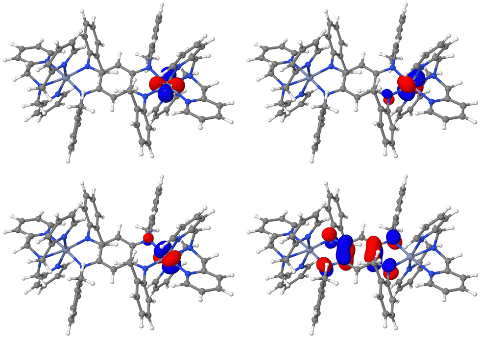
| | Fig. 2 Isosurface of the dxy (top left), dyz (top right), dyz (bottom left) and π* radical (bottom right) magnetic orbitals of 1a. Blue grey = chromium, blue = nitrogen, grey = carbon, white = hydrogen. Isovalue = 0.5 a.u. | |
 |
| | Fig. 3 Isosurface of the dxy (top left), dz2 (top right), dx2−y2 (middle left), dyz (middle right), dxz (bottom left) and π* radical (bottom right) magnetic orbitals of 2a. Purple = manganese, blue = nitrogen, grey = carbon, white = hydrogen. Isovalue = 0.5 a.u. | |
Since the orbital analysis of compounds 3a and 4a are similar, they would not be detailed in the discussion but the orbitals of both complexes may be found in Fig. S2 and S3 (ESI†).
Let us turn now to the second series of compounds featuring a semiquinone radical ligand. In this series, 3b presents a much stronger direct exchange interaction at 296 cm−1 than 4b and 5b at 109 and 111 cm−1, respectively. To explain this situation, a first observation may be done by comparing the orbital of the radical centre of the three compounds presented Fig. 4. Hence, the 3b radical orbital shows a significantly greater delocalisation tail over both magnetic centres, from which may result a stronger interaction between the radical centre and metal electrons.
 |
| | Fig. 4 Isosurface of the radical π* orbitals of 3b (top left), 4b (top right) and 5b (bottom). Orange = iron, pink = cobalt, green = nickel, blue = nitrogen, red = oxygen, grey = carbon, white = hydrogen. Isovalue = 0.5 a.u. | |
For these three compounds, a similar orbital analysis may be realised whilst the numerical contributions of every electron–electron interaction is presented in Table 3. For the sake of conciseness, let us focus on 3b since the conclusions are similar for 4b and 5b. In 3b, two t2g and two eg orbitals are singly populated due to the trigonal bipyramidal arrangement of the FeII ions. The two stronger exchange contributions are provided with the dxy and dx2−y2 orbitals due to the orientation of their lobes towards the ligand and a delocalisation tail over the oxygen atom of the bridging ligand (Fig. 5), resulting in contributions of 339 and 324 cm−1, respectively. Hence, with their orientation perpendicular to the metal–oxygen bond, the dz2 and dyz lead to two weaker contributions at 274 and 249 cm−1, respectively.
 |
| | Fig. 5 Isosurface of the dyz (top left), dz2 (top right), dx2−y2 (bottom left) and dxy (bottom right) magnetic orbitals of 3b. Orange = iron, blue = nitrogen, red = oxygen, grey = carbon, white = hydrogen. Isovalue = 0.5 a.u. | |
4.1.2 Kinetic exchange.
The kinetic exchange is the dominant contribution in both series of compounds, resulting in the antiferromagnetic nature of the metal–radical coupling. This coupling takes place between two magnetic centres of a very different nature: a radical centre bearing one unpaired electron in a rather delocalised π* orbital, and a metal ion with several unpaired electrons occupying d orbitals with a very local character. The kinetic exchange of a coupling is computed by considering two relaxations, the metal-to-radical and radical-to-metal, which thus correspond to two very different situations. Table 4 presents for both series the effective and Ũ parameters and the associated energetic contribution related to both metal-to-radical and radical-to-metal relaxations.
Table 4 Hubbard Hamiltonian and Ũ parameters and their energetic contribution (−(8SASB)−12/Ũ) for both metal → rad and metal ← rad relaxations and the resulting total kinetic exchange (ΔJKE) for all compounds in cm−1
|
|
Metal → rad |
Metal ← rad |
ΔJKE |
|
× 10−3 |
Ũ × 10−3 |
−(8SASB)−12/Ũ |
× 10−3 |
Ũ × 10−3 |
−(8SASB)−12/Ũ |
|
1a
|
−4.7 |
40.5 |
−179 |
−6.3 |
21.9 |
−606 |
−786 |
|
2a
|
−3.3 |
42.2 |
−51 |
−5.2 |
34.3 |
−152 |
−202 |
|
3a
|
−3.2 |
48.4 |
−53 |
−4.7 |
21.6 |
−259 |
−312 |
|
4a
|
−2.6 |
53.6 |
−40 |
−4.1 |
15.0 |
−371 |
−411 |
|
3b
|
−4.7 |
23.5 |
−220 |
−5.0 |
42.4 |
−146 |
−366 |
|
4b
|
−4.1 |
27.6 |
−197 |
−4.7 |
38.5 |
−194 |
−391 |
|
5b
|
−3.7 |
28.8 |
−241 |
−4.4 |
30.7 |
−318 |
−559 |
Starting with the first series, the radical-to-metal relaxation provides the strongest contribution to the total kinetic exchange with, for instance, −606 cm−1 for metal ← rad and −179 cm−1 for metal → rad in the case of 1a. For the four complexes, this difference is explained by both, a change in the t and U values. For the former, the metal ← rad t value is always stronger and this reflects the fact that it is easier for the electron to jump from the radical moiety to the metal ion than the opposite. For the U value, this parameter is for all compounds of the series smaller for metal ← rad relaxation, and the on-site repulsion energy is then smaller on the metal ion. Hence, both parameters favour the metal ← rad relaxation and explain the large discrepancy between both situations.
Regarding the energetic contribution, the second series shows different trends. Qualitatively, whilst 5b follows the trend of the first series with a larger metal ← rad relaxation, it is the opposite for 3b and both contributions are equal in 4b. Quantitatively, the metal ← rad and metal → rad relaxations provide contributions of the same order of magnitude, around a few hundred of cm−1. Going further in the Hubbard parameters, for 3b the t values from both relaxations are similar whilst both U are very different, explaining the difference between the contribution from metal → rad (−220 cm−1) and metal ← rad (−146 cm−1). For 5b the situation is the opposite since both U are similar and the different t values (−3.5 × 10⁻³ and −4.4 × 10⁻³ cm−1) explain the discrepancy between the contribution from both relaxations. It is interesting to point out that both 4b and 5bU values of the metal → rad relaxation are very similar whilst the 3b one is slightly smaller. This may be readily related to the shape of the SOMO localised on the radical ligand in Fig. 4. Indeed, as mentioned, the π* orbital of 3b is more diffused than for the other compounds and would result in weaker on-site repulsion energy.
To end this discussion, the electron–electron decomposition may be used in the context of the kinetic exchange contribution to extract the individual t and U parameters, of which the results are presented for the second series of compounds in Table 5. Let us focus on 3b since it represents a good example among all studied compounds. Unlike the direct exchange, the strongest contribution to ΔJKE is provided by the interaction between the radical centre and the dx2−y2 at −968 cm−1, followed by the interaction with the dz2 orbital at −471 cm−1. The interaction with the dxy orbital, which is the strongest for the direct exchange, is eventually the third interaction with an order of magnitude lower at −31 cm−1. This may readily be explained with the plot of the orbital in Fig. 4 and 5 for the radical ligand and the metal orbitals, respectively. Here, the lobes of the dxy orbital are in a perpendicular π arrangement to the π* of the radical centre. This situation results in an unfavourable pathway for the electron to jump from one site to the other, and this is numerically confirmed with some negligible t values below −10−3 cm−1. Finally, it may be worth noting that summing all electron–electron contributions provides an evaluation of ΔJKE in very good agreement with those from the effective and Ũ and confirms the relevance of the presented analysis.
Table 5 Hubbard Hamiltonian t and U parameters resulting from the radical–d orbital interaction, their energetic contribution (t2/U), the sum of both d → rad and d ← rad  and the total energetic contribution to the coupling
  for the second series of compounds (3–5b) in cm−1
|
|
|
t × 10−3 |
U × 10−3 |
t
2/U |

|

|
|
3b
|
dyz → rad |
— |
— |
— |
−1 |
−367 |
| dyz ← rad |
−0.2 |
37.8 |
−1 |
| dxy → rad |
−0.7 |
40.0 |
−12 |
−31 |
| dxy ← rad |
−0.8 |
31.9 |
−19 |
| dz2 → rad |
−2.5 |
28.5 |
−214 |
−471 |
| dz2 ← rad |
−3.0 |
34.5 |
−257 |
| dx2−y2 → rad |
−4.2 |
29.7 |
−582 |
−968 |
| dx2−y2 ← rad |
−3.9 |
39.5 |
−386 |
|
|
|
4a
|
dyz → rad |
— |
— |
— |
— |
−396 |
| dyz ← rad |
— |
— |
— |
| dz2 → rad |
−2.2 |
43.5 |
−111 |
−284 |
| dz2 ← rad |
−2.4 |
33.4 |
−173 |
| dx2−y2 ← rad |
−3.6 |
25.8 |
−495 |
−903 |
| dx2−y2 → rad |
−4.4 |
48.0 |
−408 |
|
|
|
5b
|
dz2 → rad |
−1.6 |
46.6 |
−52 |
−171 |
−558 |
| dz2 ← rad |
−2.0 |
33.1 |
−119 |
| dx2−y2 → rad |
−3.5 |
27.7 |
−452 |
−946 |
| dx2−y2 ← rad |
−4.5 |
40.4 |
−493 |
4.2 Modification of the radical-bridging ligands in the 1cR series
The third series of compounds with 1cO,S,OS corresponds to an interesting situation with small variations of the benzosemiquinoid-based radical ligand bridging both CrIII ions.
Let us start with the main decomposition presented in Table 2 and a comparison between the computed JΣ couplings of 1cO at −280 cm−1 and 1cS at −370 cm−1. The coupling in both compounds result from a strong direct exchange and an even larger kinetic exchange, yielding the antiferromagnetic character. However, the larger antiferromagnetic coupling in 1cS results at the same time from a weaker ferromagnetic direct exchange (107 instead of 132 cm−1 in 1cO), and a stronger antiferromagnetic kinetic exchange contribution (−461 instead of −420 cm−1). As already mentioned, whilst an averaging coupling has experimentally been determined for 1cOS, theoretically two very distinct couplings are found at −29 cm−1 for the coupling on the side of the oxygen atoms and −629 cm−1 on the side of the sulfur ones, labelled Cr(O)Rad and Cr(S)Rad hereafter, respectively. This corresponds to a strong quenching of the coupling compared to 1cO and conversely, a strong enhancement regarding 1cS. Despite this very large discrepancy, the direct exchange contributions show more moderate variations with values at 71 and 135 cm−1 for Cr(O)Rad and Cr(S)Rad, respectively. The kinetic exchange is then mainly responsible of this strong variation in JΣ with values at −101 and −741 cm−1 for Cr(O)Rad and Cr(S)Rad, respectively.
4.2.1 Direct exchange contribution.
As for 1a, the octahedral coordination in these series of CrIII-based compounds results in occupying the t2g orbitals, presented in Fig. 6, 7 and 8 for 1cO, 1cS and 1cOS, respectively. Table 6 presents the decomposition of the direct exchange into electron–electron interactions, from which the orbital analysis may be done. Regarding the similitude with 1a, only relevant aspects are detailed here. For all couplings, the interactions between the radical centre and the dxz and dyz largely dominate the overall J0 for the same reasons as for 1a. Looking at these orbitals in Fig. 6 and 7, in 1cO they show more pronounced delocalisation tails over the oxygen atoms, explaining their larger interactions at about 180 cm−1 than in 1cS at 137 and 155 cm−1. For 1cOS, the decomposition of J0 confirms a quenching of Cr(O)Rad compared to the 1cO coupling (72 instead of 132 cm−1) and an enhancement of Cr(S)Rad compared to the 1cS coupling (135 instead of 108 cm−1).
 |
| | Fig. 6 Isosurface of the dxy (top left), dxz (top right), dyz (bottom left) and radical (bottom right) magnetic orbitals of 1cO. Blue grey = chromium, blue = nitrogen, red = oxygen, grey = carbon, white = hydrogen. Isovalue = 0.5 a.u. | |
 |
| | Fig. 7 Isosurface of the dxy (top left), dyz (top right), dxz (bottom left) and radical (bottom right) magnetic orbitals of 1cS. Blue grey = chromium, blue = nitrogen, yellow = sulfur, grey = carbon, white = hydrogen. Isovalue = 0.5 a.u. | |
 |
| | Fig. 8 Isosurface of the dxy (top left), dxz (top right) and dyz (middle left) magnetic orbitals of M1(O), the dxy (middle right), dxz (bottom left) and dyz (bottom right) magnetic orbitals of M1(S), and radical orbital (bottom) in 1cOS. Blue grey = chromium, blue = nitrogen, red = oxygen, yellow = sulfur, grey = carbon, white = hydrogen. Isovalue = 0.5 a.u. | |
Table 6 Individual radical-d orbital contributions (Jd–rad0), the sum of the individual contributions (4SMSradJ0) and the total direct exchange (J0) for the third series of compounds (1cR) in cm−1
|
|
|
J
d–rad0
|
4SMSradJ0 |
J
0
|
|
1cO
|
dxy |
33 |
396 |
132 |
| dxz |
178 |
| dyz |
185 |
|
|
|
1cS
|
dxy |
31 |
323 |
108 |
| dyz |
137 |
| dxz |
155 |
|
|
|
1cOS
|
dxy(O) |
13 |
215 |
72 |
| dxz(O) |
92 |
| dyz(O) |
110 |
| dxy(S) |
51 |
405 |
135 |
| dxz(S) |
175 |
| dyz(S) |
179 |
4.2.2 Kinetic exchange contribution.
Let us turn now to the dominant kinetic exchange contribution, of which the detail of the metal-to-radical and radical-to-metal contributions and the associated and Ũ are presented in Table 7 for the three compounds. For the four involved couplings, the radical-to-metal contribution dominates the overall kinetic exchange and is approximately twice the radical-to-metal one.
Table 7 Hubbard Hamiltonian and Ũ parameters and their energetic contribution (−(8SASB)−12/Ũ) for both metal → rad and metal ← rad relaxations and the resulting total kinetic exchange (ΔJKE) for all compounds in cm−1
|
|
Metal → rad |
Metal ← rad |
ΔJKE |
|
× 10−3 |
Ũ × 10−3 |
−(8SASB)−12/Ũ |
× 10−3 |
Ũ × 10−3 |
−(8SASB)−12/Ũ |
|
1cO
|
−3.9 |
29.0 |
−174 |
−4.8 |
30.8 |
−246 |
−420 |
|
1cS
|
−3.9 |
27.8 |
−178 |
−5.4 |
34.9 |
−283 |
−461 |
|
1cOS(O) |
−1.8 |
39.2 |
−29 |
−2.4 |
26.5 |
−73 |
−101 |
|
1cOS(S) |
−4.8 |
31.5 |
−246 |
−6.4 |
27.3 |
−495 |
−741 |
Let us consider first the two symmetrical compounds 1cO and 1cS. The metal-to-radical relaxations provide similar energetic contributions at −174 and −178 cm−1, resulting from similar and Ũ parameters. Whilst the cannot be rationalised from the shape of the orbitals only, both radical orbitals seem relatively similar between 1cO and 1cS, which could result in similar Ũ. The radical-to-metal relaxation is slightly different between 1cO and 1cS and comes from different and Ũ values. Here, the t2g orbitals of 1cO show more pronounced delocalisation tails over the chalcogen atoms than in 1cS, resulting in a lower Ũ at 30.8 × 10⁻³.
Let us now focus this discussion by considering the impressive discrepancy with the kinetic exchange of both Cr(O)Rad and Cr(S)Rad couplings in 1cOS, at −101 and −741 cm−1. The small value of the Cr(O)Rad coupling results from a quenching of both metal-to-radical and radical-to-metal relaxations and oppositely, an enhancement of both makes the strong value of Cr(S)Rad. This quenching and this enhancement may be attributed to the values, driving these changes. For the metal-to-radical mechanism, whilst both Ũ regard with the radical orbital, they have different value and reflect the asymmetry of the bridging ligand.
4.2.3 Charge population analysis.
Since the differences among compounds of the third series are much smaller than the two formers, they give the opportunity to carry out a thinner investigation of the guilty for the different behaviour of the couplings in these complexes. A more quantitative analysis may be carried out using the Löwdin charge population analysis for the main atoms obtained at the HS RO stage, since it is the basis of the decomposition by defining both magnetic and core orbitals. The values are presented in Table 8 for all compounds. This analysis may be corroborated with the Ũ which is the easiest parameter to discuss since it depends almost only on the shape of the orbitals/centres themselves. In 1cS, they are two relatively localised transition metal-based magnetic centres as depicted by the large Ũ = 34.9 × 10⁻³ cm−1 and the strong charge population on the Cr ions (−2.72) and weak one on the sulfur atoms (∼0.63). Conversely, the radical centre appears rather delocalised with a small Ũ = 27.8 × 10⁻³ and the negative charge population on carbon atoms 4, 5, 6, 7, 8 and 9. In 1cO, the transition metal-based magnetic centres are more delocalised (small Ũ = 30.8 × 10⁻³ cm−1) due to the electronegativity of the oxygen atoms as shown with the smaller charge population on the Cr ions (−2.27) and larger on the oxygen ones (0.13). For this compound, the radical centre is slightly more local and presents a larger Ũ = 29.0 × 10⁻³ and positive charge population on atoms 4, 5, 8 and 9. Finally, in 1cOS, the transition metal-based magnetic centre on the oxygen atoms side (atoms 1, 2 and 3) is delocalised as shown with the small Ũ = 26.5 × 10⁻³ cm−1, small charge population on the Cr ion (−1.89) and large on the oxygen atoms (−0.11 and −0.16). The transition metal-based magnetic centre (atom 12, 11 and 10) is more localised with a slightly larger Ũ (−2.78 × 10⁻³ cm−1), more charge population on the Cr ion (−2.78) and less on the sulfur atoms (0.71 and 0.80). As a consequence, the radical centre seems to be shifted towards the sulfur atoms, with more charge population on carbon atoms 8 and 9 (−0.14).
Table 8 Atomic Löwdin charge population of the Cr ion and the main atoms of the third series computed at the high spin RO stage in atomic units
| Atoms |
1cO
|
1cS
|
1cOS
|
| 1 |
Cr |
−2.27 |
Cr |
−2.72 |
Cr |
−1.89 |
| 2 |
O |
0.13 |
S |
0.62 |
O |
−0.11 |
| 3 |
O |
0.13 |
S |
0.64 |
O |
−0.16 |
| 4 |
C |
0.15 |
C |
−0.09 |
C |
0.17 |
| 5 |
C |
0.16 |
C |
−0.07 |
C |
0.14 |
| 6 |
C |
−0.05 |
C |
−0.04 |
C |
−0.04 |
| 7 |
C |
−0.05 |
C |
−0.04 |
C |
−0.03 |
| 8 |
C |
0.16 |
C |
−0.07 |
C |
−0.14 |
| 9 |
C |
0.15 |
C |
−0.09 |
C |
−0.14 |
| 10 |
O |
0.13 |
S |
0.64 |
S |
0.71 |
| 11 |
O |
0.13 |
S |
0.62 |
S |
0.80 |
| 12 |
Cr |
−2.27 |
Cr |
−2.72 |
Cr |
−2.78 |
This analysis provides clues to rationalise the values in 1cOS. Indeed, considering the radical magnetic centre spatially closer to the sulfur atoms side of the complex, the hopping should be eased while the hopping between the radical centre and the other Cr-based centre should be more difficult. This is numerically confirmed with, for instance values at −2.4 × 10⁻³ cm−1 for Cr(S)Rad instead of −6.4 × 10⁻³ cm−1 for Cr(O)Rad in the context of radical-to-metal mechanism. Finally, this final discussion is also in line with the value of direct exchange contributions of 1cOS since the Cr(O)Rad J0 at 72 cm−1 reflects the interaction between two more distant centres than Cr(S)Rad at 135 cm−1.
5 Conclusion
In this article, we have presented the complete generalisation and first application of the decomposition/recomposition method to polynuclear systems featuring several unpaired electrons per magnetic centre. This is based on our previous work on polynuclear systems and on the newly defined effective and Ũ Hubbard Hamiltonian parameters to account for the relaxation of magnetic centres when several unpaired electrons are involved. To ease its use, we have also presented an open-source/open-access Python program to generate all determinants required to use the decomposition/recomposition method, regardless of the number of magnetic sites and unpaired electrons. Thanks to a simple input file and the previously computed and localised high spin state, the program creates a folder tree in which is generated all Orca input files. This program has been used throughout this work, allowing us to study this large number of complexes, and is available through GitLab at https://gitlab.com/gdavid123/input-files-generator.
Firstly, we applied this method to study the couplings in two series of radical-bridged dinuclear compounds, based on tetraazalene and semiquinone radical ligands, and we have shown the predominance of the direct and kinetic exchange contributions. We get insights into both contributions by decomposing them into their electron–electron interactions between the radical centre and the different d orbitals of the metal ions. This has allowed us to provide orbital analysis with numerical evaluations and we have shown the different roles of the d magnetic orbitals due to the different geometrical arrangements of both series. In addition, we have shown that in the tetraazalene-based compounds, the radical-to-metal is a much more favourable relaxation for kinetic exchange, whilst the situation is very nuanced for the semiquinone-based series.
Secondly, we used the method to investigate the influence of chemical substitution in a bis(bidentate) benzosemiquinoid radical bridging ligand in a series of chromium-based complexes. In addition to the orbital analysis, we have corroborated this study using charge population. Considering first the two symmetrical complexes, we have shown the impact of the nature of the chalcogen atoms on the definition of the magnetic centres and on the resulting coupling between them. Then, we highlighted a large discrepancy between the experimental determination and the theoretical evaluation of the asymmetrical compound. We explained the impact of the asymmetry of radical bridging ligand on the definition of the magnetic centres and the couplings between them.
Author contributions
Grégoire David carried out the conceptualisation, the implementation, performed simulations, produced the data, the formal analysis, the methodology, the supervision and all the writing process. Gwenhaël Duplaix-Rata carried out the implementation, performed simulations, produced the data and carried out the investigation. Boris Le Guennic carried out the supervision, and the validation and reviewed the paper.
Conflicts of interest
There are no conflicts to declare.
Acknowledgements
G. D. is grateful to Dr Mukesh Kumar Singh for having provided the optimised structures of the first series of compounds. The authors thank the French GENCI/IDRIS-CINES centres for high-performance computing resources. G. D. received research funding from the European Unions 843 Horizon 2020 Research and Program under Marie Skłodowska-Curie Grant Agreement No. 899546.
Notes and references
- S. Demir, I.-R. Jeon, J. R. Long and T. D. Harris, Coord. Chem. Rev., 2015, 289–290, 149–176 CrossRef CAS.
- L. Yang, J. J. Oppenheim and M. Dinca, Dalton Trans., 2022, 51, 8583–8587 RSC.
- N. Mavragani, A. A. Kitos, J. L. Brusso and M. Murugesu, Chem. – Eur. J., 2021, 27, 5091–5106 CrossRef CAS PubMed.
- S. Demir, M. I. Gonzalez, L. E. Darago, W. J. Evans and J. R. Long, Nat. Commun., 2017, 8, 2144 CrossRef.
- C. A. Gould, E. Mu, V. Vieru, L. E. Darago, K. Chakarawet, M. I. Gonzalez, S. Demir and J. R. Long, J. Am. Chem. Soc., 2020, 142, 21197–21209 CrossRef CAS PubMed.
- F. Benner, L. La Droitte, O. Cador, B. Le Guennic and S. Demir, Chem. Sci., 2023, 14, 5577–5592 RSC.
- N. Mavragani, A. A. Kitos, A. Mansikkamäki and M. Murugesu, Inorg. Chem. Front., 2023, 10, 259–266 RSC.
- S. Demir, J. M. Zadrozny, M. Nippe and J. R. Long, J. Am. Chem. Soc., 2012, 134, 18546–18549 CrossRef CAS.
- G. T. Nguyen and L. Ungur, Chem. – Eur. J., 2022, 28, e202200227 CrossRef CAS.
- J. P. Malrieu, R. Caballol, C. J. Calzado, C. de Graaf and N. Guihéry, Chem. Rev., 2013, 114, 429–492 CrossRef.
- B. O. Roos, P. R. Taylor and P. E. Siegbahn, Chem. Phys., 1980, 48, 157–173 CrossRef CAS.
- J. Miralles, O. Castell, R. Caballol and J.-P. Malrieu, Chem. Phys., 1993, 172, 33–43 CrossRef CAS.
- K. Andersson, P. A. Malmqvist, B. O. Roos, A. J. Sadlej and K. Wolinski, J. Phys. Chem., 1990, 94, 5483–5488 CrossRef CAS.
- K. Andersson, P.-Å. Malmqvist and B. O. Roos, J. Chem. Phys., 1992, 96, 1218–1226 CrossRef CAS.
- K. Andersson and B. O. Roos, Int. J. Quantum Chem., 1993, 45, 591–607 CrossRef CAS.
- C. Angeli, R. Cimiraglia, S. Evangelisti, T. Leininger and J.-P. Malrieu, J. Chem. Phys., 2001, 114, 10252–10264 CrossRef CAS.
- C. Angeli, R. Cimiraglia and J.-P. Malrieu, Chem. Phys. Lett., 2001, 350, 297–305 CrossRef CAS.
- C. Angeli, R. Cimiraglia and J.-P. Malrieu, J. Chem. Phys., 2002, 117, 9138–9153 CrossRef CAS.
- C. J. Calzado, J. Cabrero, J. P. Malrieu and R. Caballol, J. Chem. Phys., 2002, 116, 2728–2747 CrossRef CAS.
- C. J. Calzado, J. Cabrero, J. P. Malrieu and R. Caballol, J. Chem. Phys., 2002, 116, 3985–4000 CrossRef CAS.
- C. J. Calzado, C. Angeli, D. Taratiel, R. Caballol and J.-P. Malrieu, J. Chem. Phys., 2009, 131, 044327 CrossRef.
- I. de, P. R. Moreira, N. Suaud, N. Guihéry, J. P. Malrieu, R. Caballol, J. M. Bofill and F. Illas, Phys. Rev. B: Condens. Matter Mater. Phys., 2002, 66, 134430 CrossRef.
-
C. de Graaf and R. Broer, Magnetic Interactions in Molecules and Solids, Springer International Publishing, 2015 Search PubMed.
- P. Hohenberg and W. Kohn, Phys. Rev., 1964, 136, B864–B871 CrossRef.
- W. Kohn and L. J. Sham, Phys. Rev., 1965, 140, A1133–A1138 CrossRef.
- L. Noodleman, J. Chem. Phys., 1981, 74, 5737–5743 CrossRef CAS.
- A. P. Ginsberg, J. Am. Chem. Soc., 1980, 102, 111–117 CrossRef CAS.
- L. Noodleman and E. R. Davidson, Chem. Phys., 1986, 109, 131–143 CrossRef.
- L. Noodleman, C. Peng, D. Case and J.-M. Mouesca, Coord. Chem. Rev., 1995, 144, 199–244 CrossRef CAS.
- A. Bencini, F. Totti, C. A. Daul, K. Doclo, P. Fantucci and V. Barone, Inorg. Chem., 1997, 36, 5022–5030 CrossRef CAS.
- E. Ruiz, J. Cano, S. Alvarez and P. Alemany, J. Comput. Chem., 1999, 20, 1391–1400 CrossRef CAS.
- K. Yamaguchi, F. Jensen, A. Dorigo and K. Houk, Chem. Phys. Lett., 1988, 149, 537–542 CrossRef CAS.
- S. Yamanaka, M. Okumura, M. Nakano and K. Yamaguchi, J. Mol. Struct., 1994, 310, 205–218 Search PubMed.
- K. Yamaguchi, Y. Takahara, T. Fueno and K. N. Houk, Theor. Chim. Acta, 1988, 73, 337–364 CrossRef CAS.
- K. Yamaguchi, H. Fukui and T. Fueno, Chem. Lett., 1986, 625–628 CrossRef CAS.
- J. E. Peralta and J. I. Melo, J. Chem. Theory Comput., 2010, 6, 1894–1899 CrossRef CAS.
- J. J. Phillips and J. E. Peralta, J. Chem. Theory Comput., 2012, 8, 3147–3158 CrossRef CAS.
- T. Soda, Y. Kitagawa, T. Onishi, Y. Takano, Y. Shigeta, H. Nagao, Y. Yoshioka and K. Yamaguchi, Chem. Phys. Lett., 2000, 319, 223–230 CrossRef CAS.
- X. Feng and N. M. Harrison, Phys. Rev. B: Condens. Matter Mater. Phys., 2004, 70, 092402 CrossRef.
- J. J. Phillips and J. E. Peralta, J. Chem. Phys., 2011, 134, 034108 CrossRef.
- N. A. G. Bandeira and B. Le Guennic, J. Phys. Chem. A, 2012, 116, 3465–3473 CrossRef CAS.
- R. Costa, D. Reta, I. de, P. R. Moreira and F. Illas, J. Phys. Chem. A, 2018, 122, 3423–3432 CrossRef CAS.
- G. David, F. Wennmohs, F. Neese and N. Ferré, Inorg. Chem., 2018, 57, 12769–12776 CrossRef CAS.
- E. P. Kenny, G. David, N. Ferré, A. C. Jacko and B. J. Powell, Phys. Rev. Mater., 2020, 4, 044403 CrossRef CAS.
- G. Trinquier, G. David and J.-P. Malrieu, J. Phys. Chem. A, 2018, 122, 6926–6933 CrossRef CAS.
- G. Duplaix-Rata, B. Le Guennic and G. David, Phys. Chem. Chem. Phys., 2023, 25, 14170–14178 RSC.
- G. David, N. Ferré, G. Trinquier and J.-P. Malrieu, J. Chem. Phys., 2020, 153, 054120 CrossRef CAS.
- G. David, G. Trinquier and J.-P. Malrieu, J. Chem. Phys., 2020, 153, 194107 CrossRef CAS.
- G. David, N. Ferré and B. Le Guennic, J. Chem. Theory Comput., 2022, 19, 157–173 CrossRef.
- J. A. DeGayner, I.-R. Jeon and T. D. Harris, Chem. Sci., 2015, 6, 6639–6648 RSC.
- K. Chakarawet, T. D. Harris and J. R. Long, Chem. Sci., 2020, 11, 8196–8203 RSC.
- C. Hua, J. A. DeGayner and T. D. Harris, Inorg. Chem., 2019, 58, 7044–7053 CrossRef CAS.
- P. D. Loth, P. Cassoux, J. P. Daudey and J. P. Malrieu, J. Am. Chem. Soc., 1981, 103, 4007–4016 CrossRef.
- E. Coulaud, N. Guihéry, J.-P. Malrieu, D. Hagebaum-Reignier, D. Siri and N. Ferré, J. Chem. Phys., 2012, 137, 114106 CrossRef.
- E. Coulaud, J.-P. Malrieu, N. Guihéry and N. Ferré, J. Chem. Theory Comput., 2013, 9, 3429–3436 CrossRef CAS.
- F. Neese, J. Am. Chem. Soc., 2006, 128, 10213–10222 CrossRef CAS PubMed.
- M. Shoji, K. Koizumi, Y. Kitagawa, T. Kawakami, S. Yamanaka, M. Okumura and K. Yamaguchi, Chem. Phys. Lett., 2006, 432, 343–347 CrossRef CAS.
- M. K. Singh, Dalton Trans., 2020, 49, 4539–4548 RSC.
- A. D. Becke, J. Chem. Phys., 1993, 98, 5648–5652 CrossRef CAS.
- C. Lee, W. Yang and R. G. Parr, Phys. Rev. B: Condens. Matter Mater. Phys., 1988, 37, 785–789 CrossRef CAS.
- S. H. Vosko, L. Wilk and M. Nusair, Can. J. Phys., 1980, 58, 1200–1211 CrossRef CAS.
- P. J. Stephens, F. J. Devlin, C. F. Chabalowski and M. J. Frisch, J. Phys. Chem., 1994, 98, 11623–11627 CrossRef CAS.
- A. Schäfer, H. Horn and R. Ahlrichs, J. Chem. Phys., 1992, 97, 2571–2577 CrossRef.
- A. Schäfer, C. Huber and R. Ahlrichs, J. Chem. Phys., 1994, 100, 5829–5835 CrossRef.
- C. R. Groom, I. J. Bruno, M. P. Lightfoot and S. C. Ward, Acta Crystallogr., Sect. B: Struct. Sci., Cryst. Eng. Mater., 2016, 72, 171–179 CrossRef CAS.
- F. Neese, Wiley Interdiscip. Rev.: Comput. Mol. Sci., 2011, 2, 73–78 Search PubMed.
- F. Weigend and R. Ahlrichs, Phys. Chem. Chem. Phys., 2005, 7, 3297 RSC.
- X. Assfeld and J.-L. Rivail, Chem. Phys. Lett., 1996, 263, 100–106 CrossRef CAS.
-
https://www.jmol.org
.
Footnote |
| † Electronic supplementary information (ESI) available: Structures, additional orbital plots and details of calculations. See DOI: https://doi.org/10.1039/d3cp06243k |
|
| This journal is © the Owner Societies 2024 |
Click here to see how this site uses Cookies. View our privacy policy here. 
 Open Access Article
 This Open Access Article is licensed under a Creative Commons Attribution-Non Commercial 3.0 Unported Licence
 *,
Gwenhaël
Duplaix-Rata
and
Boris
Le Guennic
*,
Gwenhaël
Duplaix-Rata
and
Boris
Le Guennic

 and
and  their local spin operators, respectively. Based on the pioneering work of De Loth et al.53 and later Calzado et al.19–21 in wave-function theory, Ferré et al.54,55 and recently in a more general form David et al.47–49 decomposed in KS-DFT the magnetic exchange coupling as,
 magnetically coupled local high-spin sites labelled A, B, C, …, N, bearing nA, nB, nC, …, nN unpaired electrons, respectively, resulting in a maximum of
  couplings. To each magnetic centre is associated magnetic orbitals labelled with their lowercase letter aα, bβ, … and whose Greek letters are used for the summation over the number of unpaired electrons. Finally, i and j correspond to core orbitals, i.e. non-magnetic occupied ones, and r and s to virtual orbitals.
 direct exchange contributions,
  energy differences between the HS and some BS determinants must be defined. One may start by considering the
  configurations whose all spins of a magnetic site are flipped from the HS,RO determinant without optimising any orbital such as,


 energy differences may be defined through the BS determinants with two magnetic sites flipped as,


 direct exchange contributions may be extracted from these two sets of energy differences by solving the set of linear equations.


 energy differences from which the direct exchange is retrieved,


 and
and  to some higher-order expansion determinants. The entry of these ionic-like forms in the wavefunction results in two sets of energetic contributions,


 , α may be written in a simpler form as,


 and the total energetic contribution to the coupling
  for the second series of compounds (3–5b) in cm−1


