
 Open Access Article
 This Open Access Article is licensed under a
 Creative Commons Attribution 3.0 Unported Licence
Theory of Rayleigh–Brillouin optical activity light scattering applicable to chiral liquids
Robert P.
Cameron
 *,
Emmanouil I.
Alexakis
,
Aidan S.
Arnold
and
Duncan
McArthur
*,
Emmanouil I.
Alexakis
,
Aidan S.
Arnold
and
Duncan
McArthur
SUPA and Department of Physics, University of Strathclyde, Glasgow, G4 0NG, UK. E-mail: robert.p.cameron@strath.ac.uk
First published on 28th March 2024
Abstract
It has long been understood that dilute samples of chiral molecules such as rarefied gases should exhibit Rayleigh optical activity. We extend the existing theory by accounting for molecular dynamics and correlations, thus obtaining a more general theory of Rayleigh–Brillouin optical activity applicable to dense samples such as neat liquids.
1 Introduction
It was predicted a little over fifty years ago by Barron and collaborators that chiral molecules should exhibit Rayleigh optical activity (RayOA): differential Rayleigh scattering with respect to left- and right-handed circular polarisations of light.1–3 In the theoretical descriptions of RayOA published to date, each molecule is effectively held static in position and orientation and scattered intensities due to different molecules are added incoherently.1–11 These descriptions provide expressions for the total intensity of the analysed signal and are best suited to dilute samples such as rarefied gases in which correlations between molecules are unimportant.3,12–15In this paper, we extend the existing theory of RayOA by accounting for the translational and rotational dynamics of the molecules and adding scattered fields due to different molecules coherently, thus obtaining a more general theory that describes Rayleigh–Brillouin optical activity (RayBOA). Our theory provides expressions for not only the total intensity of the analysed signal but also the underlying frequency spectrum. It is applicable to dilute samples such as rarefied gases as well as dense samples such as neat liquids in which correlations between molecules are important.
Raman optical activity (ROA)1–3,16–18 is the inelastic sister of RayOA. The theory of ROA does not need to be extended like the theory of RayOA, however, as one can add Raman scattered intensities due to different molecules incoherently at essentially all sample densities.3,19
(Linear) RayOA is not to be confused with hyper Rayleigh optical activity (HRS OA)20–24 and its extensions,25,26 which are distinct, nonlinear optical phenomena.
For large biological scatterers, the terminology “circular intensity differential scattering” (CIDS) is often used27–31 for what is essentially RayOA.
2 Theory of RayBOA
Let us consider weak, monochromatic, off-resonant, planar light incident upon a non-conducting fluid of small, diamagnetic, chiral molecules, as illustrated in Fig. 1. Fluctuations of the optical properties within the scattering volume give rise to Rayleigh–Brillouin scattering away from the forward direction,32–54 a fraction of which is analysed at a detector in the far field. In what follows, we derive expressions for dimensionless circular spectral differentials and dimensionless circular intensity differentials which serve as convenient measures of the Rayleigh–Brillouin optical activity exhibited by the sample.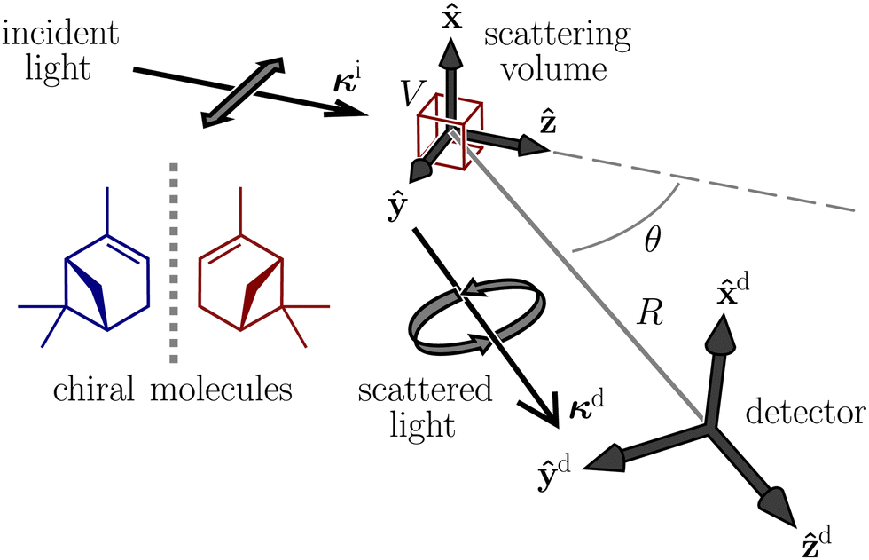 | ||
| Fig. 1 Our scattering geometry, illustrated for neat (1R,5R)-α-pinene and an SCP configuration. | ||
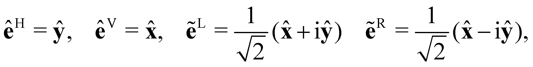
Our derivation borrows heavily from theoretical descriptions of Rayleigh–Brillouin scattering by Landau and Lifshitz12 and Berne and Pecora13 and is essentially an amalgamation of these with Barron's mechanism of Rayleigh optical activity.1–3 See also ref. 55–58. We work in an inertial frame of reference with time t and position vector r = x![[x with combining circumflex]](https://www.rsc.org/images/entities/b_char_0078_0302.gif) + yŷ + zẑ, where x, y and z are right-handed Cartesian coordinates and , ŷ and ẑ are the associated unit vectors. The Einstein summation convention is to be understood with respect to unprimed Greek indices α, β, … ∈ {x,y,z} and primed Greek indices α′,β′, … ∈ {X(n),Y(n),Z(n)}, where X(n), Y(n) and Z(n) are molecule-fixed Cartesian coordinates for the nth molecule. Complex quantities are decorated with tildes and unit vectors are decorated with carets. We use SI units throughout.
+ yŷ + zẑ, where x, y and z are right-handed Cartesian coordinates and , ŷ and ẑ are the associated unit vectors. The Einstein summation convention is to be understood with respect to unprimed Greek indices α, β, … ∈ {x,y,z} and primed Greek indices α′,β′, … ∈ {X(n),Y(n),Z(n)}, where X(n), Y(n) and Z(n) are molecule-fixed Cartesian coordinates for the nth molecule. Complex quantities are decorated with tildes and unit vectors are decorated with carets. We use SI units throughout.
2.1 The sample
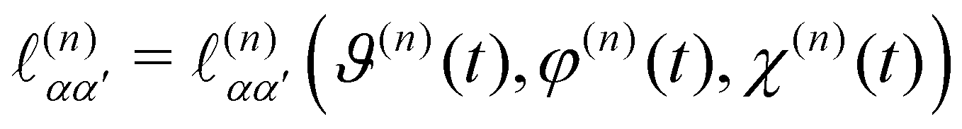
Within the scattering volume V, we model the sample as a collection of vibronically polarisable molecules that can translate with position vectors R(n) = R(n)(t) and rotate with Euler angles ϑ(n) = ϑ(n)(t), φ(n) = φ(n)(t) and χ(n) = χ(n)(t) (n ∈ {1, …}).59 In the interests of generality, we say nothing about the explicit forms of the positions and orientations of the molecules, except that they are such that the sample is optically homogeneous and isotropic on average.We take the light to satisfy Maxwell's equations in the form
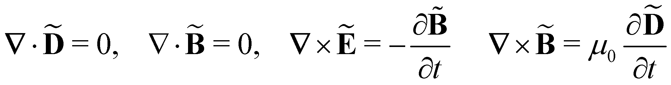 | (1) |
where
![[D with combining tilde]](https://www.rsc.org/images/entities/b_char_0044_0303.gif) = (r,t), Ẽ = Ẽ(r,t),
= (r,t), Ẽ = Ẽ(r,t), ![[B with combining tilde]](https://www.rsc.org/images/entities/b_char_0042_0303.gif) = (r,t),
= (r,t), ![[P with combining tilde]](https://www.rsc.org/images/entities/b_char_0050_0303.gif) = (r,t) and
= (r,t) and ![[M with combining tilde]](https://www.rsc.org/images/entities/b_char_004d_0303.gif) = (r,t) are the complex displacement, electric, magnetic, polarisation and magnetisation fields and ω is the angular frequency of the incident light.3,6,60
= (r,t) are the complex displacement, electric, magnetic, polarisation and magnetisation fields and ω is the angular frequency of the incident light.3,6,60
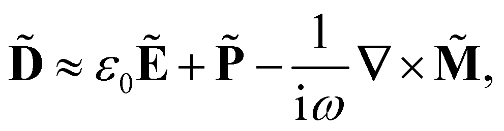
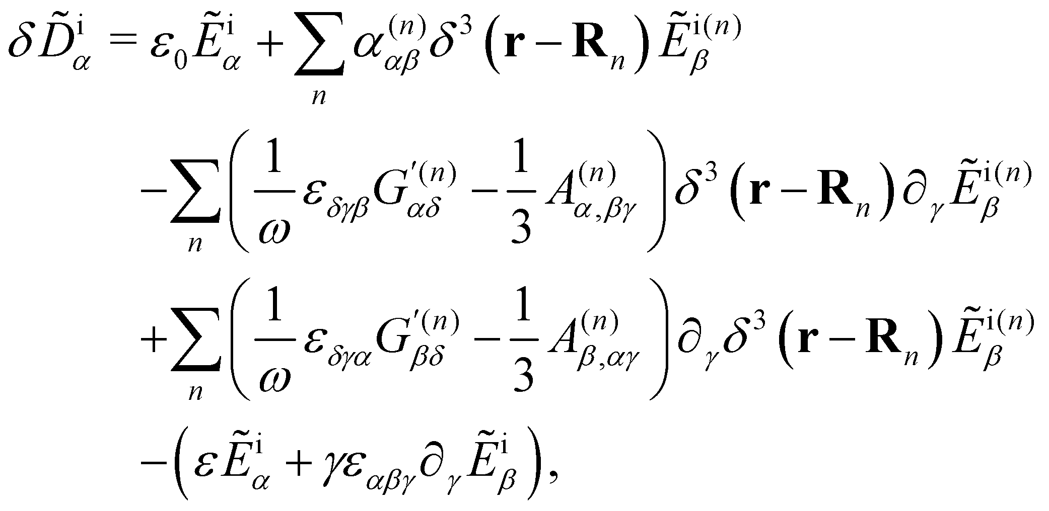
Working in the domain of linear optics to first order in multipolar expansions whilst neglecting local field corrections, we take
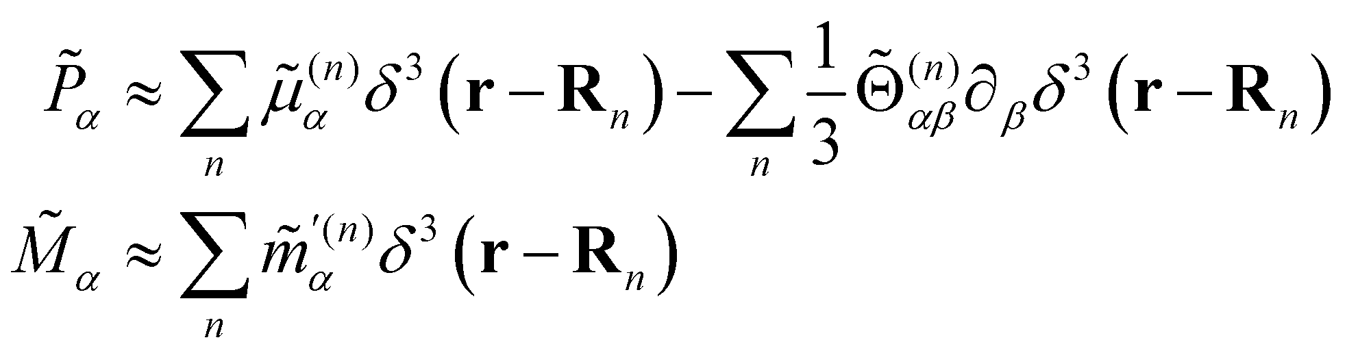
where
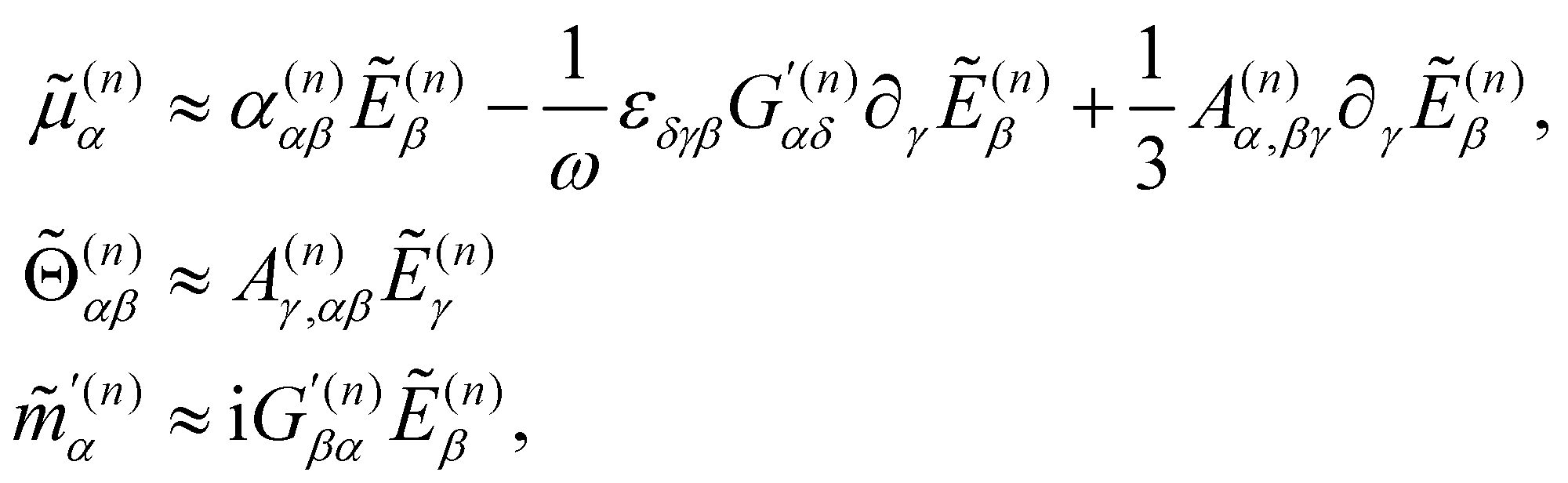
![[small mu, Greek, tilde]](https://www.rsc.org/images/entities/i_char_e0e0.gif) (n)α = (n)α(t),
(n)α = (n)α(t), ![[capital Theta, Greek, tilde]](https://www.rsc.org/images/entities/i_char_e134.gif) (n)αβ = (n)αβ(t) and
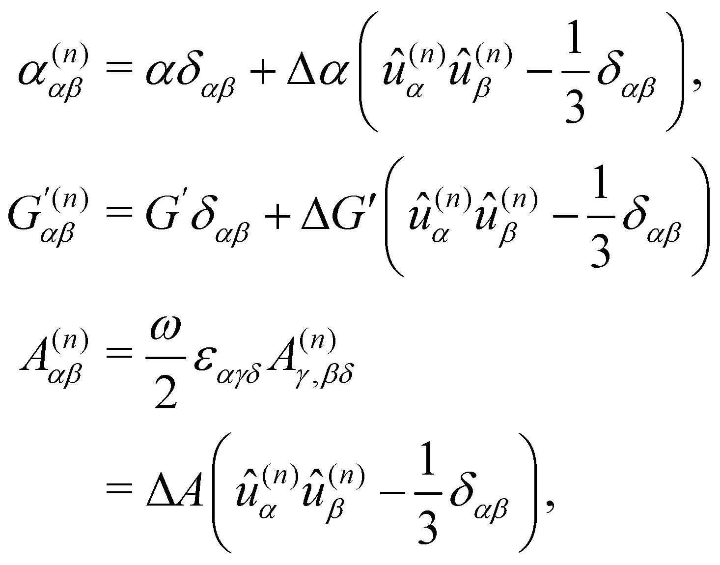
(n)αβ = (n)αβ(t) and 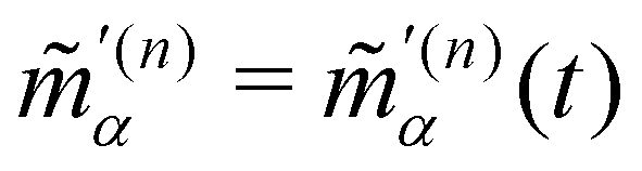 are the complex electric dipole, electric quadrupole and magnetic dipole moments of the nth molecule and α(n)αβ = α(n)βα = α(n)αβ(t),
 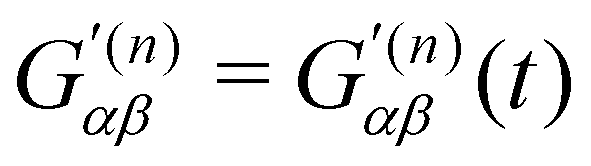 and A(n)α,βγ = A(n)α,γβ = A(n)α,βγ(t) are the vibronic† electric dipole–electric dipole, electric dipole–magnetic dipole and electric dipole–electric quadrupole polarisability tensors of the nth molecule.3,6 The laboratory-fixed components of the polarisability tensors are related to the molecule-fixed components via relations like
for example, where
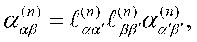
 is the direction cosine tensor for the nth molecule.3,59
2.2 Incident light
We take the incident light (superscript i) to satisfy Maxwell′s equations in the form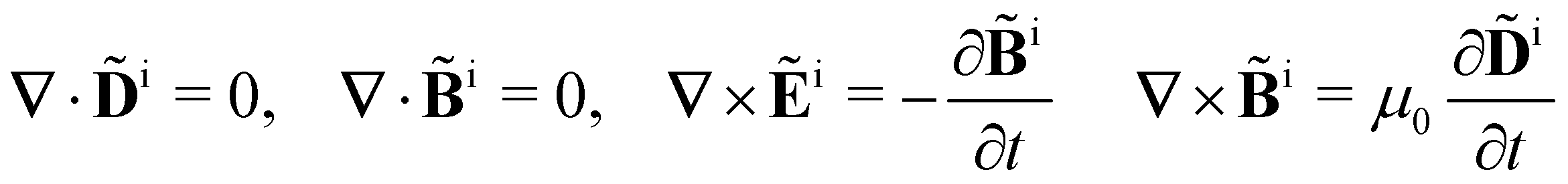 | (2) |
 | (3) |
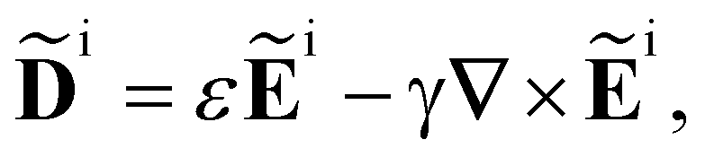
i = i(r,t), Ẽi = Ẽi(r,t), i = i(r,t) are the complex displacement, electric and magnetic fields of the incident light, ε is the average permittivity of the sample and γ is the average optical activity parameter of the sample.3,6,60 The solutions of (2) and (3) are circularly polarised plane electromagnetic waves and superpositions thereof.3
Let us assume that the incident light propagates only a short distance through the sample, as will typically be the case in an experiment using a small cuvette, for example. Accordingly, we neglect the optical rotation of the incident light (γ → 0) and take
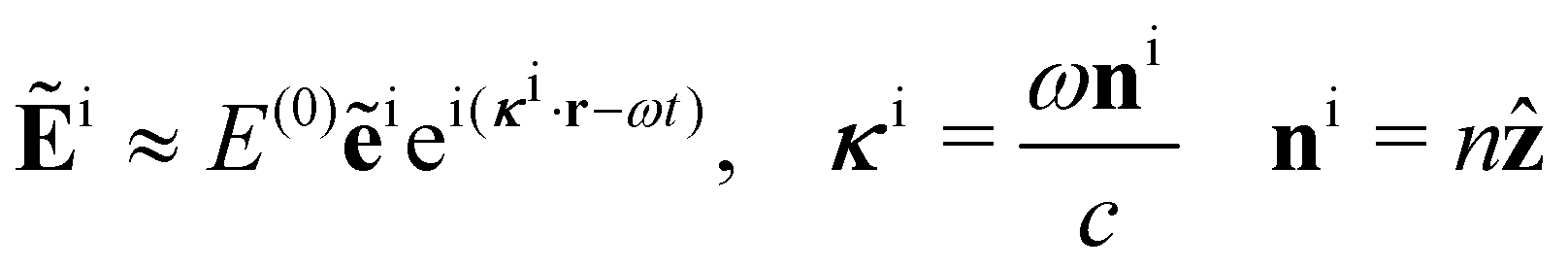
where E(0), ẽi, κi and ni are the electric-field amplitude, complex polarisation vector, wavevector and propagation vector of the incident light and
 is the average refractive index of the sample with γ = 0.
2.3 Scattered light
We take the scattered light (superscript s) to be the difference between the light and the incident light defined above, as| s = − i, Ẽs = Ẽ − Ẽi s = − i, | (4) |
s = s(r,t), Ẽs = Ẽs(r,t), s = s(r,t) are the complex displacement, electric and magnetic fields of the scattered light.12,13
Using (3) and (4), we obtain
| s ≈ εẼs − γ∇ × Ẽs + δ | (5) |
| δ ≈ − (εẼ − γ∇ × Ẽ), |
= δ(r,t) embodies fluctuations with respect to the average optical properties of the sample, being the difference between the displacement field and the form it would have if the sample had homogeneous and isotropic constitutive relations (εẼ − γ∇ × Ẽ).
Using (1), (2), (4) and (5) as well as the vector identity
| ∇ × (∇ × s) = −∇2s + ∇(∇·s), |
s must satisfy the wave equation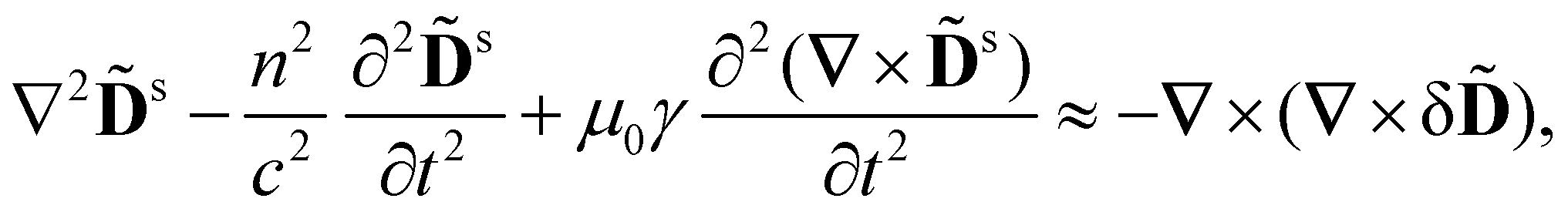 | (6) |
drive waves in the displacement s of the scattered light.
Neglecting multiple scattering,‡ we take
| δ ≈ δi | (7) |
 | (8) |
i = δi(r,t) embodies fluctuations coupled directly to the incident light.
Let us assume that the scattered light (like the incident light) propagates only a short distance through the sample. Accordingly, we neglect the optical rotation of the scattered light (γ = 0) and take the solution of (6) with (7) to be
 | (9) |
 | (10) |
i by writing δi(r′,t′) = [δi(r′,t′)exp(iωt′)]exp(−iωt′) → [δi(r′,t)exp(iωt)]exp(−iωt′), thus retaining delay for the fast dependencies only.12,13
2.4 Analysed signal at the detector
Let us focus now on the form of the scattered light at the detector (superscript d). We take the y–z plane to be the scattering plane, without loss of generality. It is convenient to introduce unit vectorsd = , ŷd = cos![[thin space (1/6-em)]](https://www.rsc.org/images/entities/char_2009.gif) θŷ − sinθẑ and ẑd = sinθŷ + cosθẑ aligned with the detector, where θ is the scattering angle.
θŷ − sinθẑ and ẑd = sinθŷ + cosθẑ aligned with the detector, where θ is the scattering angle.
As the detector lies in the far field, we take
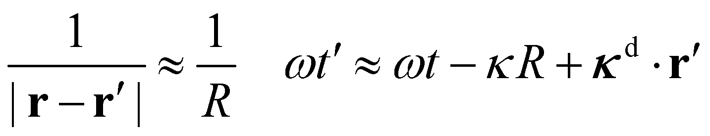 | (11) |
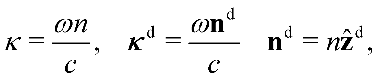 | (12) |
| −κd × (κd × V) = (κd·κd)V − κd(κd·V) |
 | (13) |
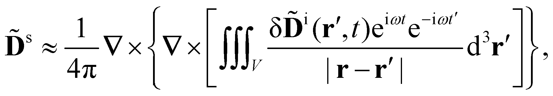
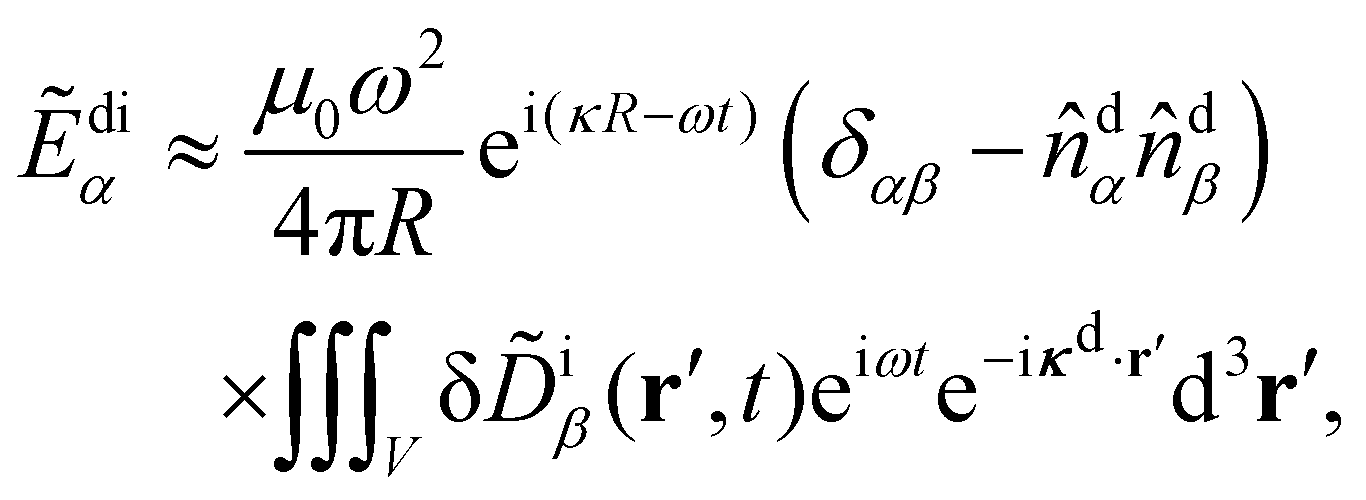
di/ε, di = di(t) being the complex displacement field of the scattered light at the detector. Substituting (8) explicitly into (13) then integrating by parts and neglecting boundary terms as well as forward-scattering contributions, we obtain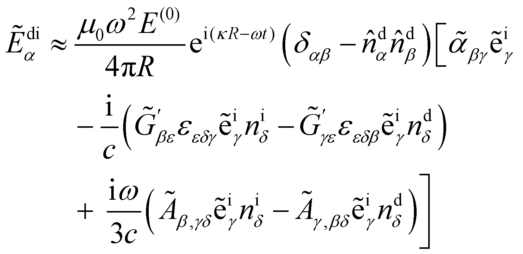 | (14) |
where
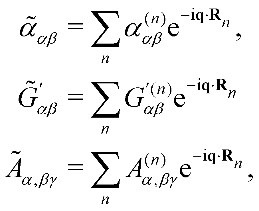
![[small alpha, Greek, tilde]](https://www.rsc.org/images/entities/i_char_e0dc.gif) αβ = αβ(t),
αβ = αβ(t), 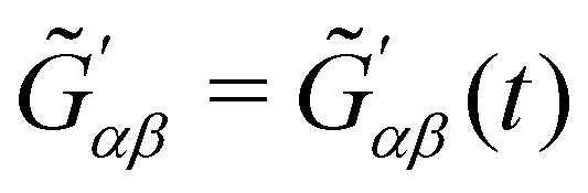 and Ãα,βγ = Ãα,βγ(t) are spatial Fourier transforms of polarisability densities, evaluated at the wavevector difference q = κd − κi ≠ 0.12,13 Note that q = |q| = 2ωnsin(θ/2)/c.
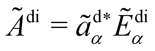
We take the analysed signal Ãdi = Ãdi(t) at the detector to be
 | (15) |
where ãd is an analysation vector that picks off the desired polarisation component of the electric field Ẽdi.
2.5 Frequency spectrum and total intensity
The frequency spectrum of the analysed signal Ãdi can be calculated as the temporal Fourier transform of the autocorrelation of Ãdi, as
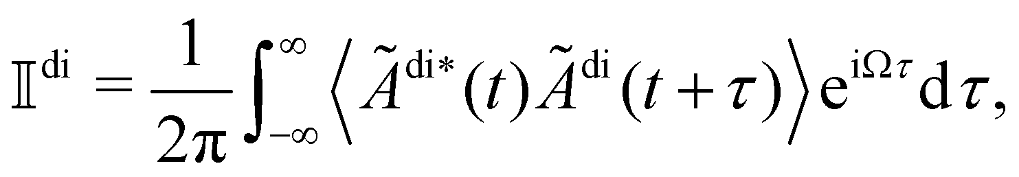 | (16) |
 , as
, asNote that
 for Ω < 0, assuming that Ãdi = 0 for Ω < 0.
Substituting (14) and (15) into (16) whilst working to first order in multipolar expansions, we obtain
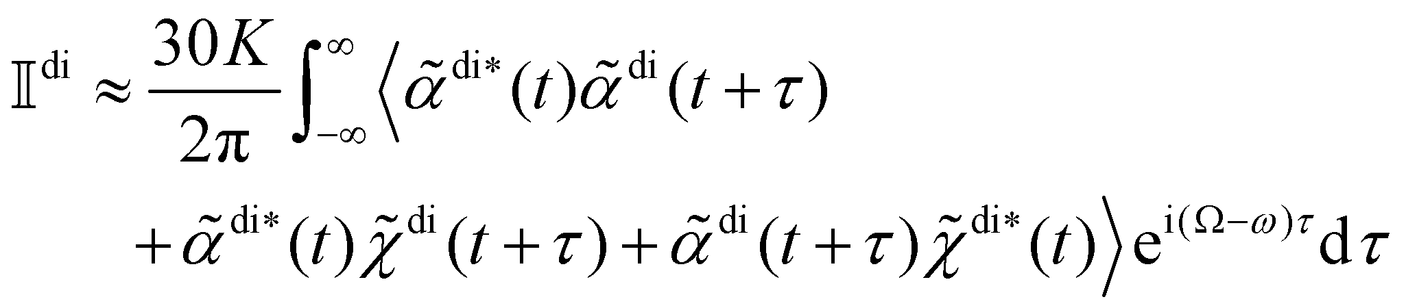 | (17) |
where K is a prefactor that contains the usual ω4, E(0)2 and 1/R2 scalings characteristic of Rayleigh scattering in the far field and
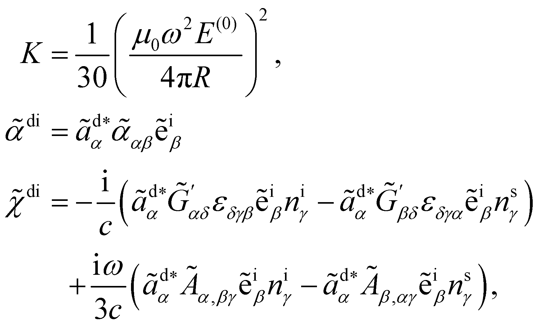 di = di(t) and
 ![[small chi, Greek, tilde]](https://www.rsc.org/images/entities/i_char_e11b.gif) di = di(t) are convenient shorthands.
di = di(t) are convenient shorthands.
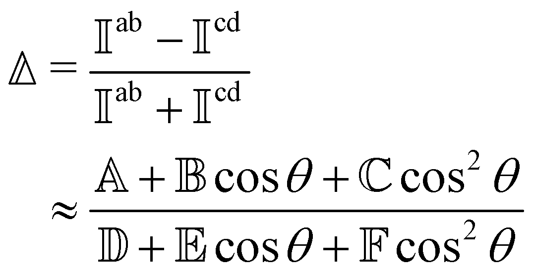
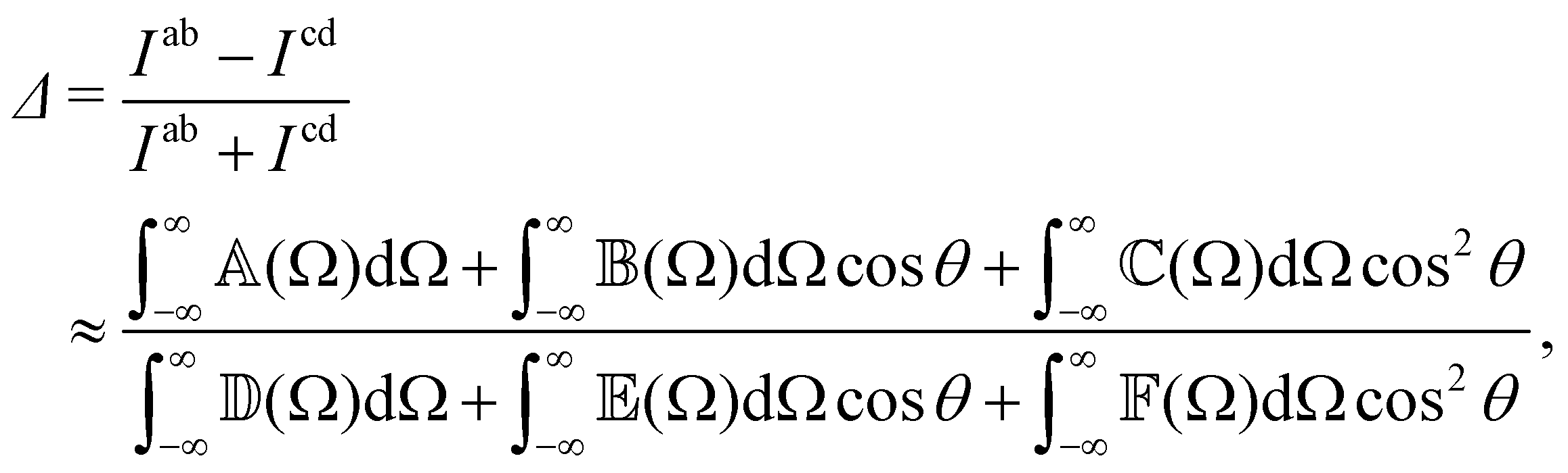
2.6 Dimensionless circular spectral and intensity differentials
RayOA (and by extension RayBOA) can manifest as an intensity difference with respect to left- and right-handed circular polarisation states in the scattered light (scattered circular polarisation or SCP),1 the incident light (incident circular polarisation or ICP)2 or both simultaneously (dual circular polarisation or DCPI).64As convenient measures of RayBOA, we identify dimensionless circular spectral differentials  of the form
 | (18) |
 | (19) |
 ,
,  ,
,  ,
,  ,
,  and
and  are coefficients that depend on the specific configuration being considered. Substituting (17) into (18) and (19) and making use of basic symmetry arguments, we obtain the results listed in Table 1 with
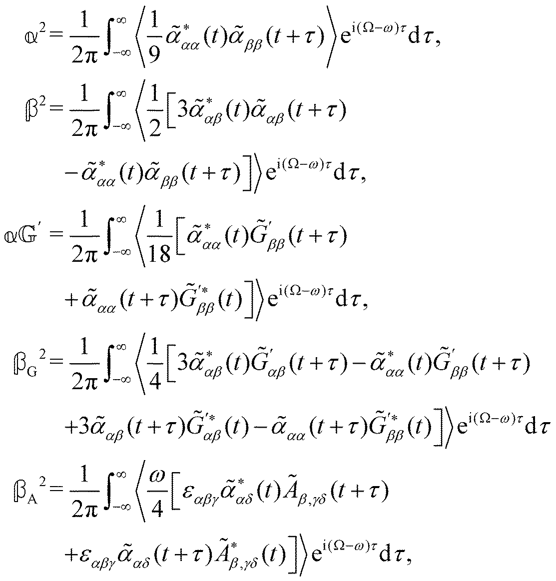 | (20) |
 accounts for isotropic electric dipole-electric dipole scattering,
 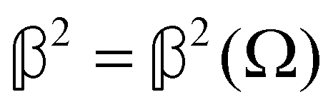 accounts for anisotropic electric dipole-electric dipole scattering,
 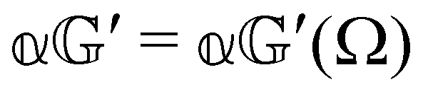 accounts for isotropic electric dipole–magnetic dipole scattering,
  accounts for anisotropic electric dipole–magnetic dipole scattering and
 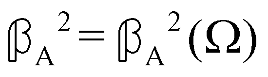 accounts for anisotropic electric dipole-electric quadrupole scattering. Note that
  and
and  are chirally insensitive whereas
  ,
,  and
and  have equal magnitudes but opposite signs for enantiomorphic samples. It follows that both
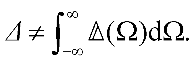
  and Δ have equal magnitudes but opposite signs for enantiomorphous samples, thus serving as signatures of chirality.
| a | b | c | d |
|
|
|
|
|
|
|---|---|---|---|---|---|---|---|---|---|
| R | H | L | H |

|

|
|
|
0 |
|
| R | V | L | V |
|

|
0 |
|
0 | 0 |
| R | N | L | N |

|

|
|

|
0 |
|
| H | R | H | L |
|

|

|

|
0 |

|
| V | R | V | L |
|
|
0 |

|
0 | 0 |
| N | R | N | R |
|

|

|

|
0 |
|
| R | R | L | L |
|
|
|
|
|

|
Let us emphasise here that the circular differentials  and Δ are not simply related to each other, in particular that
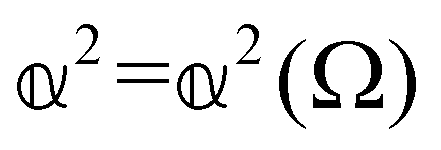
As a quick check on the validity of our results, we note that for the special case of a single molecule held fixed at the origin, we have 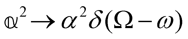 ,
, 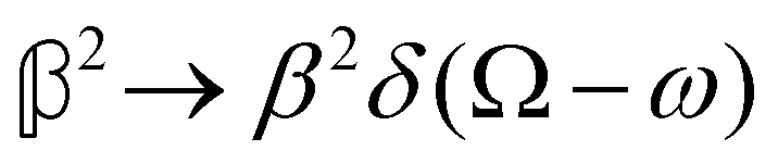 ,
, 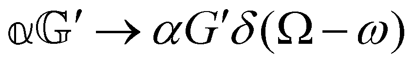 ,
,  and
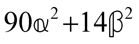
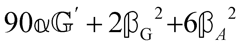
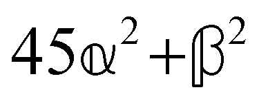
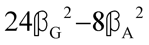
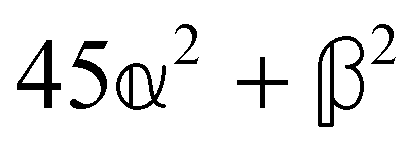
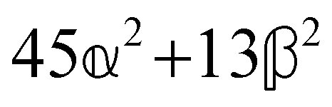
and  , where α2, β2, αG′, βG2 and βA2 are the usual single-molecule invariants.3,7 This sees our results for the circular intensity differentials Δ reduce immediately to the (rotationally averaged) results reported previously elsewhere,2–4,7 as they should.
3 Toy model
For the sake of illustration, let us now evaluate the circular differentials and Δ for a toy model of an enantiopure neat liquid. This model is not meant to provide accurate predictions for real liquids. Rather, we include it to demonstrate the mathematical extraction of spectra, the explicit application of our theory to real liquids being a challenging task that we will return to in future publications.
Considering molecules with quasi-cylindrical symmetry for the sake of simplicity, we take
 | (21) |
with

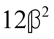
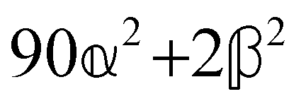
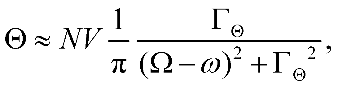
where α2, β2, αG′, β2 = Δα2, βG2 = ΔαΔG′ and βA2= 2ΔαΔA/3 are the usual single-molecule invariants3,7 and S = S(Ω) and Θ = Θ(Ω) are dynamic structure factors.13,65
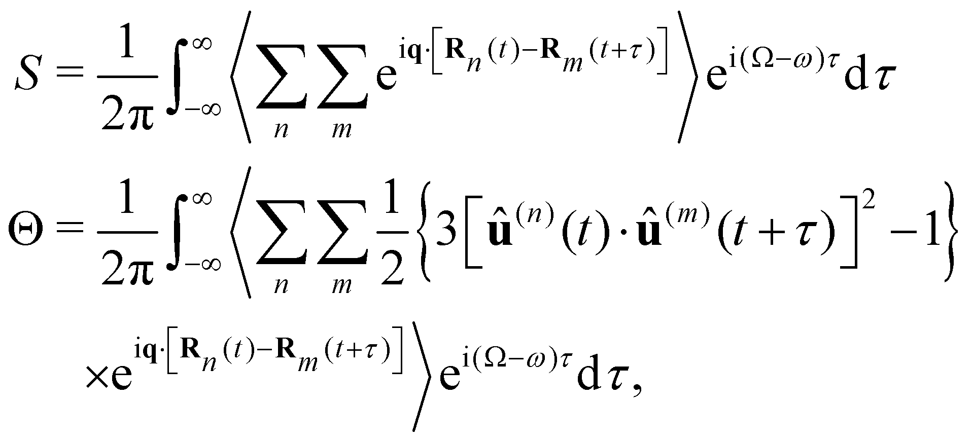
A simple hydrodynamic model (neglecting intramolecular relaxation) gives
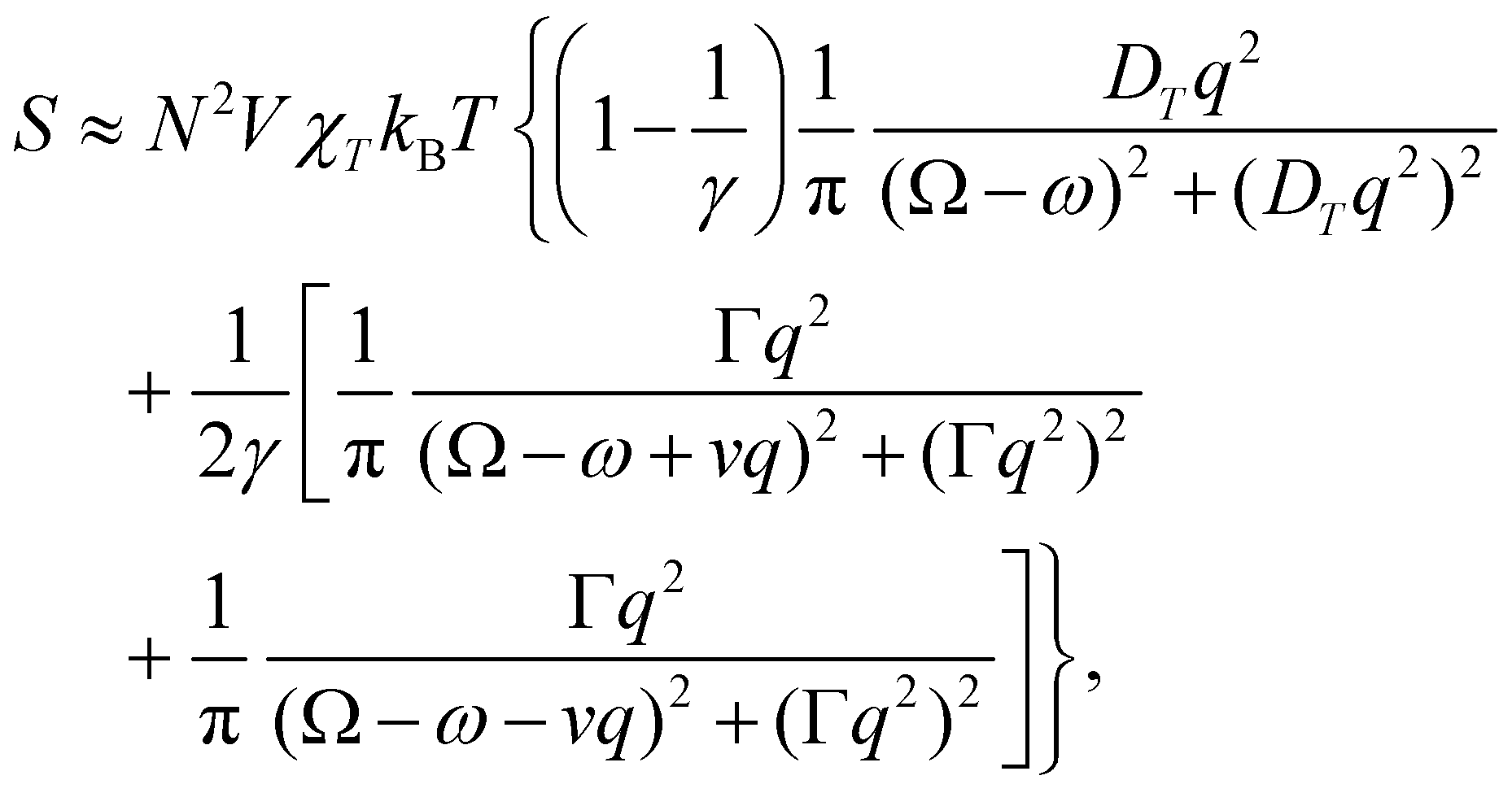
where ΓΘ is a tumbling rate.13,66 The time-domain molecular dynamics that underpin these forms for S and Θ are described explicitly in ref. 12, 13, 15, 54 and 66.
Focussing on a right-angled SCP configuration with vertically polarised incident light for the sake of concreteness, we have
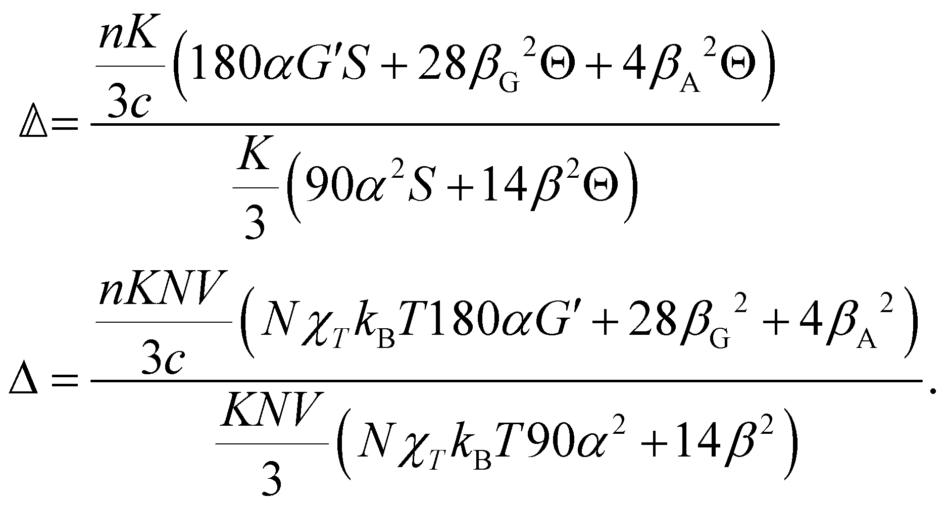
 offers more information than Δ in that the isotropic and anisotropic contributions can be distinguished as a function of the angular frequency Ω. In the limiting case where ΓΘ ≫ vq ≫ Γq2 > DTq2, we find in particular that
Using typical values,7 this leads us to predict that

although considerable variation is possible, of course.

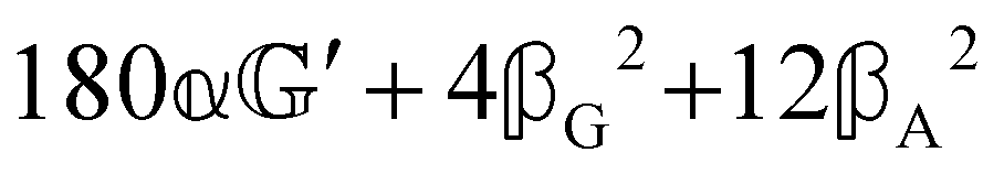
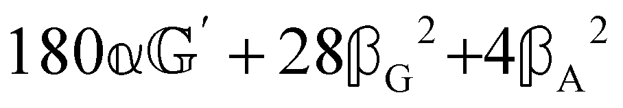
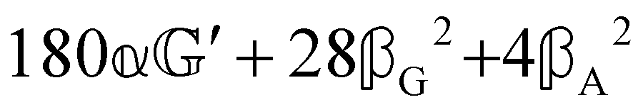
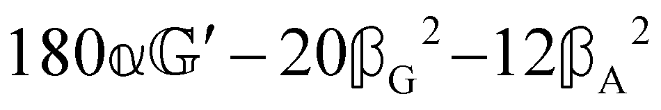
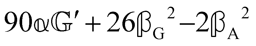
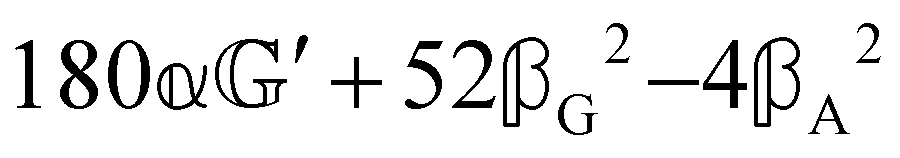
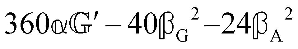
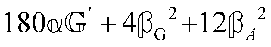
These features are illustrated in Fig. 2 for ω = 3.54 Prad s−1, n = 1.40, γ = 1.33, NχTkBT = 0.100, DTq2/2π = 80.0 MHz, vq/2π = 3.00 GHz, Γq2/2π = 160 MHz, ΓΘ/2π = 10.0 GHz, β2 = 0.100α2, αG′/c = ±1.00 × 10⁻⁵α2 and βG2/c = βA2/c = ±1.00 × 10⁻⁴α2, where the upper and lower signs correspond to opposite enantiomers. The circular spectral sum  (i.e. the spectrum of the S0 Stokes parameter of the scattered light3) is positive and consists of a narrow Gross (centre) line53,54 and narrow Brillouin lines40,45,46,53 superposed with a broad Rayleigh wing.47–52 The circular spectral difference
  (i.e. the spectrum of the S3 Stokes parameter of the scattered light3) has opposite signs for opposite enantiomers, appearing inverted at the Gross and Brillouin lines as we have taken 180αG′ and 28βG2 + 4βA2 to have opposite relative signs. The resulting circular spectral differential also has opposite signs for opposite enantiomers and appears inverted at the Gross and Brillouin lines, where it is suppressed in magnitude in accord with our prediction above.
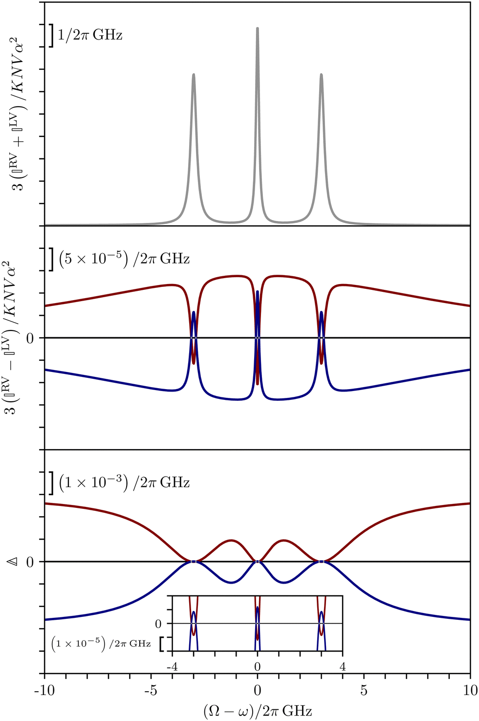 | ||
| Fig. 2 Circular spectra predicted for a toy model of an enantiopure neat liquid. The red and blue curves correspond to opposite enantiomers. | ||
4 Conclusions
We have presented a theory of RayBOA applicable to dense samples such as neat liquids. There are many possible avenues for future research.We have evaluated the circular differentials for a toy model of an enantiopure neat liquid. It remains for us to consider more realistic models for a variety of different samples. Molecular dynamics simulations have recently been applied with success to ROA19,67,68 and might be developed for RayBOA as well.
We have adopted a microscopic approach, facilitating comparison with the existing theory of RayOA.1–11 A macroscopic approach is also possible12,13,15,37,39 and might yield new insights. Care will need to be taken with the choice of macroscopic constitutive relations,69,70 which must include electric dipole–electric quadrupole contributions to describe RayBOA correctly even for isotropic samples.
We have focussed on SCP, ICP and DCPI RayBOA for off-resonant illumination of a fluid by planar light. Interesting new features should emerge for illumination near resonance,5,64,71,72 anisotropic samples5 and illumination by structured light.8,10,11,73 It should also prove fruitful to consider the influence of static magnetic fields,74 static electric fields31,75 and higher-order multipolar contributions.9,28
A particularly interesting question is whether Rayleigh–Brillouin optical activity can be used to detect chiral (acoustic) phonons in appropriate samples.19,76–78
Although our focus in this paper has been on small molecules, similar ideas can be developed for larger scatterers, including large biomolecules.27–31
We will return to these and related tasks elsewhere.
Conflicts of interest
There are no conflicts to declare.Acknowledgements
The authors gratefully acknowledge support from the Royal Society (URF\R1\191243) and EPSRC (EP/R513349/1). We thank Laurence Barron for useful discussions. RPC is a Royal Society University Research Fellow. For the purpose of open access, the authors have applied a Creative Commons Attribution (CC BY) licence to any Author Accepted Manuscript (AAM) version arising from this submission.References
- P. W. Atkins and L. D. Barron, Mol. Phys., 1969, 16, 453–466 CrossRef CAS.
- L. D. Barron and A. D. Buckingham, Mol. Phys., 1971, 20, 1111–1119 CrossRef CAS.
- L. D. Barron, Molecular Light Scattering and Optical Activity, Cambridge University Press, 2004 Search PubMed.
- D. L. Andrews, J. Chem. Phys., 1980, 72, 4141–4144 CrossRef CAS.
- L. Hecht and L. D. Barron, Chem. Phys. Lett., 1994, 225, 525–530 CrossRef CAS.
- D. P. Craig and T. Thirunamachandran, Molecular Quantum Electrodynamics: An Introduction to Radiation Molecule Interactions, Dover Publications, 1998 Search PubMed.
- G. Zuber, P. Wipf and D. N. Beratan, ChemPhysChem, 2008, 9, 265–271 CrossRef CAS PubMed.
- R. P. Cameron and S. M. Barnett, Phys. Chem. Chem. Phys., 2014, 16, 25819–25829 RSC.
- R. P. Cameron and N. Mackinnon, Phys. Rev. A, 2018, 98, 013814 CrossRef CAS.
- K. A. Forbes, Phys. Rev. Lett., 2019, 122, 103201 CrossRef CAS PubMed.
- K. A. Forbes and D. L. Andrews, Phys. Rev. Res., 2019, 1, 033080 CrossRef CAS.
- L. D. Landau, E. M. Lifshitz and L. P. Pitaevskii, Electrodynamics of Continuous Media, Pergamon Press, 1984 Search PubMed.
- B. J. Berne and R. Pecora, Dynamic Light Scattering with Applications to Chemistry, Biology, and Physics, Dover Publications, 2000 Search PubMed.
- I. I. Sobel'man, Phys.-Uspekhi, 2002, 45, 75–80 CrossRef.
- R. W. Boyd, Nonlinear Optics, Academic Press, 2003 Search PubMed.
- L. D. Barron and M. P. Bogaard, J. Am. Chem. Soc., 1973, 95, 603–605 CrossRef CAS.
- W. Hug, S. Kint, G. F. Bailey and J. R. Scherer, J. Am. Chem. Soc., 1975, 97, 5589–5590 CrossRef CAS.
- S. O. Pour, L. D. Barron, S. T. Mutter and E. W. Blanch, Chiral Analysis: Advances in Spectroscopy, Chromatography and Emerging Methods, Elsevier, 2nd edn, 2018, ch. 6, pp. 249–291 Search PubMed.
- P. Michal, J. Kapitán, J. Kessler and P. Bour, Phys. Chem. Chem. Phys., 2022, 24, 19722–19733 RSC.
- D. L. Andrews and T. Thirunamachandran, J. Chem. Phys., 1979, 70, 1027–1030 CrossRef CAS.
- J. T. Collins, K. R. Rusimova, D. C. Hooper, H.-H. Jeong, L. Ohnoutek, F. Pradaux-Caggiano, T. Verbiest, D. R. Carbery, P. Fischer and V. K. Valev, Phys. Rev. X, 2019, 9, 011024 CAS.
- D. Verreault, K. Moreno, E. Merlet, F. Adamietz, B. Kauffmann, Y. Ferrand, C. Olivier and V. Rodriguez, J. Am. Chem. Soc., 2020, 142, 257–263 CrossRef CAS PubMed.
- L. Ohnoutek, N. H. Cho, A. W. A. Murphy, H. Kim, D. M. Rasadean, G. D. Pantos, K. T. Nam and V. K. Valev, Nano Lett., 2020, 20, 5792–5798 CrossRef CAS PubMed.
- L. Ohnoutek, B. J. Olohan, R. R. Jones, X. Zheng, H.-H. Jeong and V. K. Valev, Nanoscale, 2022, 14, 3888–3898 RSC.
- L. Ohnoutek, H.-H. Jeong, R. R. Jones, J. Sachs, B. J. Olohan, D.-M. Rasadean, G. D. Pantos, D. L. Andrews, P. Fischer and V. K. Valev, Laser Photonics Rev., 2021, 15, 2100235 CrossRef CAS.
- L. Ohnoutek, J.-Y. Kim, J. Lu, B. J. Olohan, D. M. Rasadean, G. D. Pantos, N. A. Kotov and V. K. Valev, Nat. Photonics, 2022, 16, 126–133 CrossRef CAS.
- M. F. Maestre, C. Bustamante, T. L. Hayes, J. A. Subirana and I. Tinoco Jr., Nature, 1982, 298, 773–774 CrossRef CAS PubMed.
- I. Tinoco Jr. and A. L. Williams Jr., Ann. Rev. Phys. Chem., 1984, 35, 329–355 CrossRef.
- A. L. Gratiet, R. Marongiu and A. Diaspro, Polymers, 2020, 12, 2428 CrossRef PubMed.
- Y.-L. Pan, A. Kalume, J. Arnold, L. Beresnev, C. Wang, D. N. Rivera, K. K. Crown and J. Santarpia, Opt. Express, 2022, 30, 1442–1451 CrossRef CAS PubMed.
- S. Gassó and K. D. Knobelspiesse, Atmos. Chem. Phys., 2022, 22, 13581–13605 CrossRef.
- J. W. Strutt, Philos. Mag., 1871, 41, 107–120 Search PubMed.
- J. W. Strutt, Philos. Mag., 1871, 41, 274–279 Search PubMed.
- J. W. Strutt, Philos. Mag., 1871, 41, 447–454 Search PubMed.
- L. Rayleigh, Philos. Mag., 1881, 12, 81–101 Search PubMed.
- L. Rayleigh, Philos. Mag., 1899, 47, 375–384 Search PubMed.
- M. Smoluchowski, Ann. Physik., 1908, 25, 205–226 CrossRef.
- L. Rayleigh, Nature, 1910, 83, 48–50 CrossRef.
- A. Einstein, Ann. Physik., 1910, 338, 1275–1298 CrossRef.
- L. Brillouin, C. R. Acad. Sci., 1914, 158, 1331–1334 Search PubMed.
- J. Cabannes, C. R. Acad. Sci., 1915, 160, 62–63 CAS.
- R. J. Strutt, Proc. Roy. Soc., 1918, A95, 155–176 Search PubMed.
- L. Rayleigh, Philos. Mag., 1918, 35, 373–381 Search PubMed.
- J. Cabannes, Ann. Phys., 1921, 15, 5–150 Search PubMed.
- L. Brillouin, Ann. Phys., 1922, 9, 88–122 Search PubMed.
- L. Mandelstam, Zh. Russ. Fiz-Khim. Ova, 1926, 58, 381–391 Search PubMed.
- J. Cabannes, C. R. Acad. Sci., 1928, 186, 1201–1202 CAS.
- J. Cabannes and P. Daure, C. R. Acad. Sci., 1928, 186, 1533–1534 CAS.
- C. V. Raman and K. S. Krishnan, Nature, 1928, 122, 278 CrossRef CAS.
- J. Cabannes and Y. Rocard, J. Phys. Radium, 1929, 10, 52–71 CrossRef CAS.
- C. Manneback, Z. Physik, 1930, 62, 224–252 CrossRef CAS.
- C. Manneback, Z. Physik, 1930, 65, 574 CrossRef.
- E. Gross, Nature, 1930, 126, 201–202 CrossRef.
- L. Landau and G. Placzek, Phys. Z. Sowjet, 1934, 5, 172–173 CAS.
- I. I. Komarov and I. Z. Fisher, Sov. Phys. JETP, 1963, 16, 1358–1361 Search PubMed.
- A. T. Young, Appl. Opt., 1981, 20, 533–535 CrossRef CAS PubMed.
- A. T. Young, Phys. Today, 1982, 35, 42–48 CrossRef CAS.
- I. L. Fabelinskii, Phys.-Usp., 1994, 37, 821–859 CrossRef.
- P. R. Bunker and P. Jensen, Fundamentals of Molecular Symmetry, IOP Publishing, 2005 Search PubMed.
- J. D. Jackson, Classical Electrodynamics, Wiley, 1998 Search PubMed.
- L. Rayleigh, Philos. Mag., 1900, 49, 324–325 Search PubMed.
- R. S. Krishnan, Proc. Indian Acad. Sci., 1938, 7, 21–34 CrossRef.
- F. Perrin, J. Chem. Phys., 1942, 10, 415–427 CrossRef CAS.
- L. A. Nafie and T. B. Freedman, Chem. Phys. Lett., 1989, 154, 260–266 CrossRef CAS.
- L. van Hove, Phys. Rev., 1954, 95, 249–262 CrossRef CAS.
- P. Debye, Polar Molecules, Dover, 1929 Search PubMed.
- M. Brehm and M. Thomas, J. Phys. Chem. Lett., 2017, 8, 3409–3414 CrossRef CAS PubMed.
- Y. Yang, J. Cheramy, M. Brehm and Y. Xu, ChemPhysChem, 2022, 23, e202200161 CrossRef CAS PubMed.
- S. M. Barnett and R. P. Cameron, J. Opt., 2016, 18, 015404 CrossRef.
- R. Ossikovski, O. Arteaga and C. Sturm, Adv. Photonics Res., 2021, 2, 2100160 CrossRef.
- L. D. Barron and J. R. Escribano, Chem. Phys., 1985, 98, 437–446 CrossRef CAS.
- L. Hecht and L. A. Nafie, Chem. Phys. Lett., 1990, 174, 575–582 CrossRef CAS.
- D. McArthur, A. M. Yao and F. Papoff, Phys. Rev. Res., 2020, 2, 013100 CrossRef CAS.
- L. D. Barron and A. D. Buckingham, Mol. Phys., 1972, 23, 145–150 CrossRef CAS.
- A. D. Buckingham and R. E. Raab, Proc. R. Soc. Lond. A, 1975, 345, 365–377 Search PubMed.
- H. Zhu, J. Yi, M.-Y. Li, J. Xiao, L. Zhang, C.-W. Yang, R. A. Kaindl, L.-J. Li, Y. Wang and X. Zhang, Science, 2018, 359, 579–582 CrossRef CAS PubMed.
- W. J. Choi, K. Yano, M. Cha, F. M. Colombari, J.-Y. Kim, Y. Wang, S. H. Lee, K. Sun, J. M. Kruger, A. F. de Moura and N. A. Kotov, Nat. Photonics, 2022, 16, 366–373 CrossRef CAS.
- H. Ueda, M. Garcia-Fernández, S. Agrestini, C. P. Romao, J. van den Brink, N. A. Spaldin, K.-J. Zhou and U. Staub, Nature, 2023, 618, 946–950 CrossRef CAS PubMed.
Footnotes |
| † By “vibronic”, we mean simply that the polarisabilities account for electromagnetic perturbation of the vibrational and electronic degrees of freedom of the molecules. The initial and final states in the polarisabilities are taken to be the same; the molecules do not undergo real vibronic transitions. |
| ‡ The condition 4πμ02ω4α2NV1/3 ≪ 1 should be well satisfied in the visible domain by typical small-molecule liquids for a cuvette of volume V = 1 cm3, say. |
| This journal is © the Owner Societies 2024 |