
 Open Access Article
 This Open Access Article is licensed under a
 Creative Commons Attribution 3.0 Unported Licence
Benchmarking non-adiabatic quantum dynamics using the molecular Tully models†
Sandra
Gómez
 a,
Eryn
Spinlove
bc and
Graham
Worth
*c
a,
Eryn
Spinlove
bc and
Graham
Worth
*c
aDepartamento de Química Física, Universidad de Salamanca, 37008, Spain Web: https://ror.org/02f40zc51
bFaculty of Science and Engineering, Theoretical Chemistry – Zernike Institute for Advanced Materials, Nijenborgh 4, 9747 AG, Groningen, The Netherlands
cDepartment of Chemistry, University College London, 20 Gordon St, London WC1H 0AJ, UK. E-mail: g.a.worth@ucl.ac.uk
First published on 8th December 2023
Abstract
On-the-fly non-adiabatic dynamics methods are becoming more important as tools to characterise the time evolution of a system after absorbing light. These methods, which calculate quantities such as state energies, gradients and interstate couplings at every time step, circumvent the requirement for pre-computed potential energy surfaces. There are a number of different algorithms used, the most common being Tully Surface Hopping (TSH), but all are approximate solutions to the time-dependent Schrödinger equation and benchmarking is required to understand their accuracy and performance. For this, a common set of systems and observables are required to compare them. In this work, we validate the on-the-fly direct dynamics variational multi-configuration Gaussian (DD-vMCG) method using three molecular systems recently suggested by Ibele and Curchod as molecular versions of the Tully model systems used to test one-dimensional non-adiabatic behaviour [Ibele et al., Phys. Chem. Chem. Phys. 2020, 22, 15183–15196]. Parametrised linear vibronic potential energy surfaces for each of the systems were also tested and compared to on-the-fly results. The molecules, which we term the Ibele–Curchod models, are ethene, DMABN and fulvene and the authors used them to test and compare several versions of the Ab Initio Multiple Spawning (AIMS) method alongside TSH. The three systems present different deactivation pathways after excitation to their ππ* bright states. When comparing DD-vMCG to AIMS and TSH, we obtain crucial differences in some cases, for which an explanation is provided by the classical nature and the chosen initial conditions of the TSH simulations.
1 Introduction
It is a known problem in research that a set of accepted standard test systems are required to validate and assess new methods. Methods to describe non-adiabaticity, or processes happening in the vicinity of conical intersections, were derived first in the late 1980s for pre-computed potential energy surfaces (PES).1–3 In 1990 Tully proposed three 1-dimensional, 2-state model potentials for testing non-adiabatic dynamics methods.1 The single avoided crossing, dual avoided crossing and extended coupling with reflection surfaces exhibit three challenging features to dynamics methods. While these test systems continue to be used for initial testing of dynamics methods, whether surface hopping or full quantum dynamics, this is dependant upon simulations being performed upon pre-calculated potential energy surfaces. Comprehensive insights into methods using pre-computed PES, both based on trajectories and grids, can be found in ref. 4–6.The requirement of pre-computed PES is a significant bottleneck for dynamics calculations. In 1973, I. S. Y. Wang and M. Karplus published a communication describing a study of the approach of H2 towards CH2.7 Their simulations showed that rotation of the H2 was involved and hence structures away from the minimum energy path towards the formation of CH4 are required. In this method, the CNDO model8,9 was employed for calculating required structures as needed along the trajectory thus bypassing the requirement for pre-computed potentials. It is hence the first example of an on-the-fly, or direct, dynamics method. Leforestier, in 1978,10 calculated the on-the-fly reaction dynamics of the nucleophilic substitution H− + CH4 → CH4 + H−. Using GTOs, provided by Gaussian 70,11 for the electronic structure and gradient calculations, he showed that the reaction occurs via a non-adiabatic path involving the vibration of methane. Helgaker et al. improved on this idea in a study of CH2+ + H2.12 It was, however, not until 1994 that the modern formalism of on-the-fly, non-adiabatic dynamics was developed for dynamics in a manifold of electronic states. A collaborative effort between the groups of Robb, Olivucci and Schlegel made it possible to use classical trajectories hopping within electronic states and computing electronic structure quantities along the dynamics.13
An important consideration in the development of direct dynamics-based methods is the capabilities of the computational resources at hand when conducting simulations. Since Wang and Karplus's work in 1973, there has been substantial progress in computational power encompassing both processing speed and memory capacity. The direct comparison of the speed of computer systems across decades is challenging due to changes in computational architecture. However, as an illustration, Leforestier reported that a gradient calculation using a 4-31G basis set took 30.85 minutes,10 while the same calculation on the computer system used in this work took 1.5 seconds. The computer used by Leforestier had an advertised maximum storage capacity of 8 MB,14 while the databases alone generated by the dynamics calculations in this work are 85.8 GB. It is readily evident, from a practical perspective, that modern HPC facilities are required for performing direct dynamics simulations.
The recent advancements in constructing experimentally viable on-the-fly methodologies for non-adiabatic dynamics therefore aligns with the field's emerging status. Several methods are currently under development, and among them, the following are of particular significance: ab initio multiple spawning (AIMS),15 direct dynamics variational multi-configuration Gaussian (DD-vMCG),16 Multi Configurational Ehrenfest (MCE),17 as well as ab initio surface hopping implementations in the Newton X18 and SHARC19 software packages. Descriptions of the methods presently under development are available in ref. 20–22.
As a consequence of the diverse approaches to direct dynamics, complications arise from both the attainable results as well as the way in which these results can be illustrated. These differences can, broadly, be placed into three categories. The first is that the surface hopping and multiple spawning approaches are carried out in the adiabatic picture while vMCG is in the diabatic picture, leading to non-comparable state populations. The second issue arising relates to the structures, in terms of properties and timescales, along the trajectories of the dynamics. In the spawning and surface hopping methods, properties are averaged over the trajectories while in the DD-vMCG and MCE methods, there is a weighted average. The third issue arising pertains to the representation of the potential energies experienced by the evolving system. In AIMS/TSH, the potential surfaces are only known along each trajectory as a set of time-ordered values. In contrast, the database obtained in DD-vMCG provides global potential energy surfaces that can be analysed and post-processed. These issues pose a significant challenge in the comparison of the results obtained from the different methods. Within the direct non-adiabatic dynamics community there is a consensus that not only is a common set of test systems required, but also a mutually accepted approach to the representation of the dynamical results.
In 2020, Ibele and Curchod23 published a novel set of candidates for testing on-the-fly non-adiabatic dynamic methods. In the present work, we follow their suggestions and test our direct dynamics method, DD-vMCG, on the three molecular systems proposed. In their classification, ethene resembled the Tully model I, since it seemed to present one simple non-adiabatic event. 4-N,N-Dimethylaminobenzonitrile (DMABN) was proposed as molecular Tully model II, since its dynamics showed multiple passages through the intersection seam due to the near-degeneracy of the two electronic states involved. Furthermore, in the dynamics of the DMABN molecule, the ground electronic state remains inactive, as the molecule exhibits fluorescence, and non-radiative processes are confined to the upper (excited) electronic surfaces, making this system easier to treat with TD-DFT. A reflection back towards the same region from which it initially relaxed was found in fulvene, therefore it was assigned to Tully model III. To take the focus away from a comparison to the Tully models, we shall name them the Ibele–Curchod (IC) models and refer to the ethene system as IC1, DMABN as IC2 and fulvene as IC3. The potential surfaces and short-time dynamics of ethene,24–28 fulvene29–31 and DMABN32,33 have all been studied at various levels of theory. The IC models thus need to be defined by a particular level of electronic structure theory and initial starting geometry, which will be detailed below. The models are thus not chosen to be the best possible representation of the actual molecules, but are chosen for efficiency and non-adiabatic behaviour.
Another interesting matter arising from the IC models is the characterisation of the types of conical intersection. The topography of intersections are usually classified as either peaked or sloped.34 The former results in a fast motion away from the intersection, while the latter leads to re-crossing. It was concluded by Ibele and Curchod that the topography of the identified conical intersection of DMABN was peaked, whereas the population in fulvene passed through a sloped conical intersection.
As will be shown in this paper, the passage through a conical intersection is dominated not only by its topography but also how it is accessed. We introduce the following terms to describe how the intersections are accessed. “Direct” is when the intersection can be reached directly from the Franck–Condon point along the vibrational modes initially excited by the photo-excitation. “Indirect” is when the energy has to flow from the initially excited modes to other modes in order for the intersection to be accessed. The descriptor “Immediate” will also be used in place of direct for when the intersection is so close to the Franck–Condon point that it lies under the initially excited wavepacket. In the following we will see that the three models cover these three categories (indirect, immediate, direct), with distinctive population dynamics.
In the following, the three test systems will be studied using DD-vMCG as well as the DD-TSH implementation in the Quantics software package. Comparisons will also be made with full quantum dynamics on the related linear vibronic coupling (LVC) model Hamiltonians, providing a solid benchmark. As well as demonstrating the utility of the benchmark systems, this study is a snapshot of the present capabilities of the DD-vMCG method. A key feature of the work is that the same potentials are used for all nuclear dynamics methods to allow a rigorous comparison. Differences seen in the results from the TSH and vMCG simulations, however, highlight the problem of comparing calculations made in different representations (diabatic for vMCG and adiabatic for TSH), as well as the need for complete quantum dynamics benchmarks.
2 The Ibele–Curchod models
The main aim of this paper is to set up the three models introduced by Ibele and Curchod23 as standard tests for non-adiabatic direct dynamics simulations. A key part of models used for benchmarking is a clear definition of the parameters needed for calculations. The level of quantum chemistry and the states included in the models are given below.IC1: ethene. SA(3)-CASSCF(2/2)/6-31G* with the π and π* orbitals in the active space. Three states are included in the dynamics (N, V and Z in Mulliken notation35). Ibele and Curchod included only two states. However, there are three states in the state averaged CAS, and all three states are found to be active in the dynamics so they must be included.
IC2: DMABN. TDA-ωB97X-D3/cc-pVDZ within the TD-DFT framework. The three lowest states are included in the dynamics (S0, Lb, La).
IC3: fulvene. SA(3)-CASSCF(6/6)/6-31G* including three pairs of π and π* orbitals in the active space. The lowest two states are included in the dynamics (S0 and S1 (ππ*)).
The propagation for all models starts with a vertical excitation at the Franck–Condon point to the brightest excited state (S1 in IC1 and IC3, S2 for IC2). The initial wavepacket is constructed as the ground state vibrational wavefunction in the harmonic approximation of the ground state potential surface placed on the chosen electronic state. Data from the quantum chemistry calculations (optimised geometry, ground state frequencies and state energies at the Franck–Condon point) for all three models are given in the ESI,† for reference.
It should be noted that the electronic structure chosen for IC1 and IC3 is the same as in ref. 23, while for IC2 we have chosen to use the functional benchmarked in a recent study on DMABN33 in place of the LC-PBE functional used in the original work. The IC2 calculation used the electronic structure code Q-Chem36 which allows computing analytic non-adiabatic couplings with TD-DFT, and Molpro37–39 was used for IC1 and IC3.
3 Methodology
In this work, three methods were used for the propagation of the nuclei: multi-configuration time-dependent Hartree (MCTDH), variational multi-configuration Gaussian (vMCG) and Tully surface hopping (TSH). All are well described in the literature and only brief overviews will be given here. All dynamics calculations were made using the Quantics Package.40,41The Quantics code is able to generate a range of initial wavefunctions and links to a number of potential routines that can be input as text files for analytical functions, such as the vibronic coupling Hamiltonian used here. It also has interfaces to a number of quantum chemistry codes for direct dynamics, including Molpro and Q-Chem used here. The direct dynamics interface works via a “quantum chemistry database”, referred to in this work as “the QC database”, or merely “the database”. As a propagation proceeds, the energies, gradients and non-adiabatic couplings are calculated and stored as a set of points. Hessians are calculated only at the first point and provided at all other points in the database by a Hessian updating scheme. A new point is added to the database whenever the configuration on a trajectory is a pre-defined distance away from any point in the database. In these calculations the measure of difference was that any atom was displaced by more than 0.2 Bohr from any point in the database. For the DD-vMCG simulations, the data was transformed to the diabatic picture using the propagation diabatisation scheme, which ensures that the model diabatic potentials reproduce the adiabatic potentials from the quantum chemistry.42 Global surfaces are then provided by Shepard interpolation between the points in the smoother diabatic picture. Adiabatic surfaces are provided by diagonalising the interpolated diabatic potentials rather than interpolating the quantum chemistry data. Details of the DD-vMCG scheme are given in ref. 43.
Both MCTDH and vMCG are parts of the core implementation of the Quantics code. The surface hopping calculations utilise an interface between Quantics and a general surface hopping code written by Sapunar and Došlić,44 referred to here as Zagreb SH. This interface has been introduced in a previous study on the non-adiabatic dynamics of the butatriene cation and cyclohexadiene.45
3.1 Multi-configuration time-dependent Hartree (MCTDH)
MCTDH is a complete, grid-based solution of the nuclear time-dependent Schrödinger equation. The wavefunction ansatz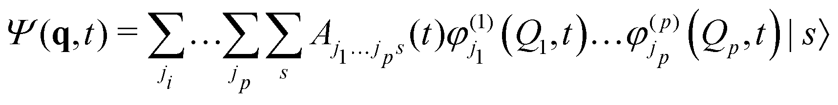 | (1) |
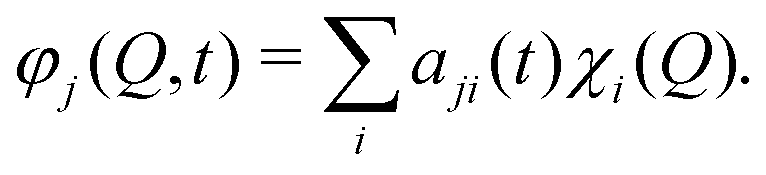 | (2) |
Equations of motion for the expansion coefficients and SPFs are obtained from a variational principle to ensure that the basis set remains optimally small. For details see ref. 3 and 47. MCTDH is a convergent method that provides the numerically exact solution to the TDSE for the given Hamiltonian. It does, however, require the potential functions to be known globally before the calculations are made, i.e., pre-computed. For efficiency, the potential also has to be in a “sum-of-products” form
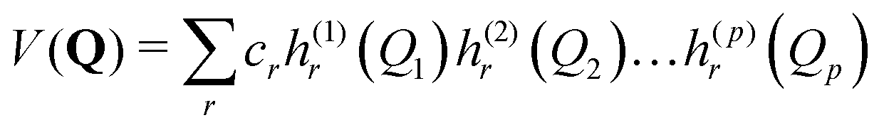 | (3) |
For large systems, typically more than 12 degrees of freedom, it is necessary to use the multi-layer formalism in which the SPFs of eqn (1) are recursively expanded in functions of MCTDH form to reduce the dimensionality before expanding in the DVR.48–50 ML-MCTDH has enabled calculations with many hundreds of degrees of freedom, still ensuring convergence to the numerically exact solution for the given Hamiltonian.
3.2 Variational multi-configuration Gaussian (vMCG)
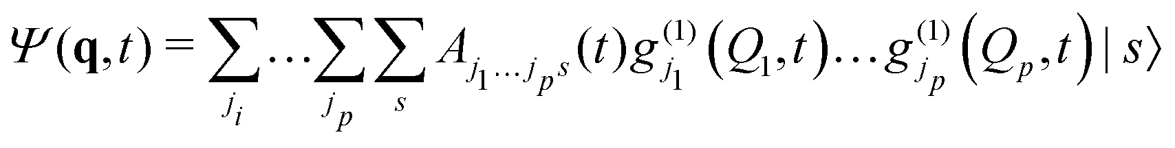
The vMCG method writes the wavefunction as a superposition of Gaussian basis functions (GBFs)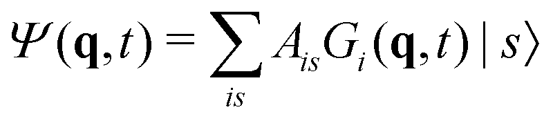 | (4) |
gi(qα,t) = exp(σi,αqα2 + ξqi![[thin space (1/6-em)]](https://www.rsc.org/images/entities/char_2009.gif) α + ζi). α + ζi). | (5) |
| gi(qα) = exp(−Ai(qα − qiα,0)2 + ipiα,0(qα − qiα,0) + iγi) | (6) |
![[thin space (1/6-em)]](https://www.rsc.org/images/entities/i_char_2009.gif) α,0 and piα,0 correspond to the width, centre coordinate of the Gaussian function and momentum of that centre, respectively.
α,0 and piα,0 correspond to the width, centre coordinate of the Gaussian function and momentum of that centre, respectively.
Solving the TDSE using the vMCG ansatz, eqn (4), and the Dirac-Frenkel variational principle, leads to equations of motion for the expansion coefficients and GBF parameters. These equations provide trajectories followed by the GBFs. However, these are not classical, as in the Heller formalism, since the GBFs are variationally coupled, leading to faster convergence with basis set size. Integrals of the Hamiltonian in the GBF basis sets 〈gi|H|gj〉 are required, and if these are evaluated exactly, the method converges to a numerically exact solution of the TDSE, just like MCTDH. However, while MCTDH breaks the problem down to low-dimensional integrals that can be solved using quadrature, here we have highly multi-dimensional integrals. To solve these, we use a local harmonic approximation (LHA) to the potential surfaces and the integrals over the potentials 〈gi|V|gj〉 use the potential expanded around the centre of the GBF on the right hand side of the integral to second order:
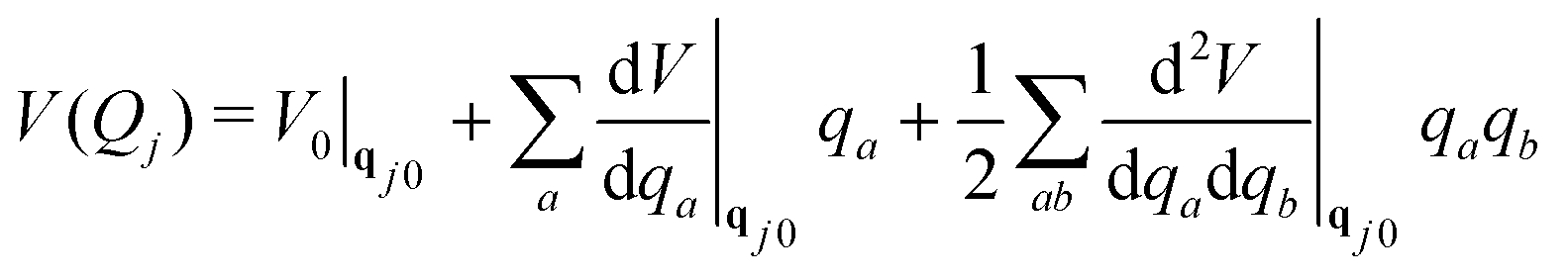 | (7) |
Unfortunately, the coupling between GBFs leads to equations of motion that require the inversion of a matrix at every step in a propagation that is (n × N)2, where n is the number of degrees of freedom and N the number of Gaussian functions. This becomes expensive for large systems but the effort can be alleviated by partitioning the system and using a product basis
 | (8) |
 | (9) |
 | (10) |
The equations of motion for the expansion coefficients and GWP parameters are propagated using a variable time-step Runge–Kutta integration scheme. The inversion of the overlap and C-matrix also lead to numerical noise in the propagation and the wavefunction is renormalised every 1 fs to enhance stability.
3.3 Trajectory surface hopping (TSH)
The TSH calculations used the classic “fewest switches” algorithm1 and the trajectories were propagated with a time-step of 0.1 fs. Hopping probabilities were computed from analytically obtained non-adiabatic couplings and isotropic velocity scaling was used to conserve energy. A known problem of TSH is its overcoherence: since trajectories follow the gradient of the active state, population transfer may occur as if parts of the wavepacket were moving in the same direction with the same velocity in an unphysical manner. To overcome this, a simple and commonly used methodology exists, whereby exponential damping of the amplitude of the other states (which are following the active state gradient) is performed, depending on the kinetic energy and the energy gap. This is the energy-based decoherence (EDC) scheme of Grannucci et al.,54 which is also the standard in the Zagreb SH code.Using the Quantics–Zagreb SH interface ensures that the TSH calculations run on the same potentials as the vMCG and MCTDH calculations.45 The initial conditions can also be chosen to be as similar as possible. In these calculations, the swarm of trajectories are initialised by sampling from a Wigner distribution of the ground state vibrational eigenstate used in the vMCG and MCTDH simulations using the same normal mode coordinates to define the harmonic approximation. The trajectories are then propagated in mass-weighted normal mode coordinates to remove the centre of mass motion, as done in the wavepacket methods. One major difference, however, is that the vertical excitation, in TSH is to the adiabatic rather than diabatic excited state.
The equations of motion are propagated using a velocity Verlet algorithm with a time step of 0.5 fs.
3.4 State populations
To compare vMCG results to TSH, the diabatic populations obtained directly from vMCG dynamics must be converted to the adiabatic picture. To do so, the expectation value of the adiabatic projection operator in terms of the diabatic states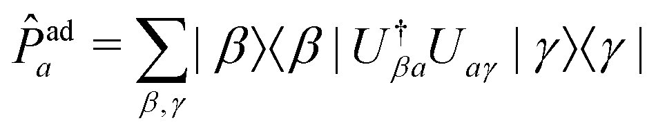 | (11) |
| U†(q)W(q)U(q) = V(q) | (12) |
 | (13) |
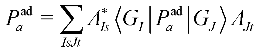
This expression requires the evaluation of multi-dimensional integrals over the GWP basis functions, prohibitive for the size of systems treated here. Making use of the local nature of these functions, a practical scheme can be obtained using the saddle-point approximation, in which the integral value is taken at the central points of the Gaussians multiplied by the overlaps. To reduce the number of operations further, these are evaluated using the average position of the Gaussian centres
| 〈Gi(Q)|P|Gj(q)〉 = 0.5(〈Gi|Gj〉Pada(qi0) + 〈Gi|Gj〉Pada(qj0)) | (14) |
3.5 Procedure
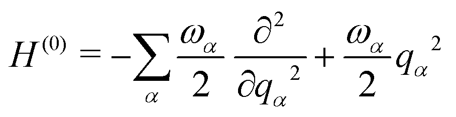
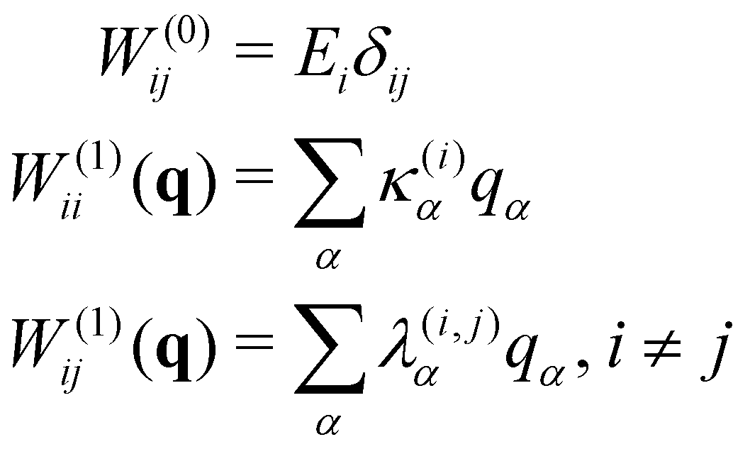
The starting point for the calculations was to construct a Linear Vibronic Coupling (LVC) Model Hamiltonian for the 3 systems.55,56 This model is an analytical description of the coupled potentials around the Frank–Condon (FC) region which can be used by the MCTDH method for an accurate description of the early-time dynamics. These simulations provide a rigorous check of the performance of the vMCG and TSH calculations at the early stages, along with a basic classification of the conical intersections directly accessible by the IC systems studied.The LVC model assumes a diabatic electronic basis and describes the diabatic potentials and state couplings as Taylor expansions around the Franck–Condon (FC) point. The coordinates are dimensionless (mass-frequency scaled) normal modes, taken from the ground electronic state at the equilibrium geometry. For an N-state system the LVC is written as an N × N matrix
| H = H(0)1 + W(0) + W(1) | (15) |
 | (16) |
 | (17) |
One could improve the model by using the calculated Hessians to provide on-diagonal second-order terms. A Quadratic Vibronic Coupling Model (QVC) is, however, much more expensive due to the large number of additional terms. It also rarely provides more than minor changes to population dynamics and for these model systems, test calculations showed that indeed the QVC results are very similar to those from the LVC.
In order to speed up the calculations, the vMCG basis functions were partitioned into two parts, i.e. the G-MCTDH scheme of eqn (9) was used. The modes in each partition were selected using the LVC model parameters as guidance. If a mode has an on-diagonal linear, κ, parameter then it is a tuning mode that has a gradient at the FC point and modulates the gap between the surfaces. The importance of the mode is given by the ratio κ/ω as this defines how far a harmonic oscillator is shifted from the FC point. If a mode has an off-diagonal linear parameter, λ, then it is a coupling mode that provides the non-adiabatic coupling between electronic states. Again its importance is given by the ratio λ/ω.
After analysis of the importance of the modes, IC2 had the strongest 29 modes in the first partition and the remaining in the second. IC3 had 12 modes in the first partition. This first partition in both cases required more GWPs for convergence as it contains the modes with strong coupling and hence more anharmonic surfaces. For IC1, ethene is small enough to simply divide into 2 parts comprising six modes each. The vMCG partitioning and final basis sets are given in Table 1. Details of the ML-MCTDH trees showing the structure and number of basis functions needed for convergence of the MCTDH calculations are given in the ESI.†
| Model | DD-vMCG | DD-TSH | |||
|---|---|---|---|---|---|
| System partitioning | N GBF | Energy (eV) | N traj | Energy (eV) | |
| IC1 | ν 5, ν6, ν7, ν8, ν9, ν10 | 40 | 12.331 ± 0.191 | 490 | 11.502 ± 0.090 |
| ν 1, ν2, ν3, ν4, ν11, ν12 | 40 | ||||
| IC2 | ν 1, ν19, ν3, ν46, ν33, ν34, ν35, ν45, ν31, ν32, ν36, ν8,ν23, ν47, ν44, ν12, ν6, | 40 | 10.093 ± 0.114 | 477 | 11.072 ± 0.005 |
| ν 11, ν2, ν14, ν9, ν5, ν22, ν13, ν30, ν41, ν29, ν10, ν4, ν42, ν43, ν27, ν25, ν57, | |||||
| ν 17, ν18, ν49, ν40, ν54 | |||||
| ν 39, ν7, ν28, ν15, ν53, ν55, ν21, ν26, ν37, ν16, ν38, ν20, ν24, ν48, ν50, ν51, | 30 | ||||
| ν 52, ν56 | |||||
| IC3 | ν 22, ν9, ν24, ν19, ν6, ν15, ν13, ν17, ν20, ν21, ν25, ν30 | 80 | 6.862 ± 0.091 | 479 | 6.856 ± 0.003 |
| ν 2, ν18, ν14, ν23, ν16, ν29, ν3, ν8, ν12, ν4, ν10, ν11, ν1, ν7, ν28, ν26, ν5, ν27 | 40 | ||||
Simulations on the LVC Hamiltonians for all 3 systems using ML-MCTDH, vMCG and 500 TSH trajectories were run for 100 fs and state populations obtained. ML-MCTDH and vMCG provide diabatic populations, so adiabatic populations were obtained from the vMCG calculations using the saddle-point procedure described above to compare to the TSH results.
Starting with the potential surfaces provided by the linear vibronic coupling model, direct dynamics calculations were run on the three models using the DD-vMCG and DD-TSH methods. Normal mode coordinates were used for all simulations, with the same coordinates used for each system. The vMCG (both DD-vMCG and vMCG on the LVC models) simulations used mass-frequency scaled coordinates, while the TSH used mass-scaled coordinates so as to ensure that the kinetic energy operator has the Cartesian form required by the surface hopping code. All results are displayed in mass-frequency scaled coordinates. The data in the databases is taken directly from the quantum chemistry, and stored, in Cartesian coordinates, hence interpolations take place in this coordinate system. A simple linear transformation connects the normal mode and Cartesian representations.
The initial conditions for the vMCG calculations are defined using the ground-state wavefunction in the harmonic approximation. The GWP centred at the FC point has an initial population of 1, while all others have a population of 0. The unpopulated GWPs are then distributed in momentum space, stepping out from the zero momentum sequentially along each degree of freedom. The initial conditions for the TSH calculations are set such that the initial wavepacket is randomly sampled, using a Wigner distribution, in order to prepare the swarm. Consequently, the calculations have the same initial conditions.
For each system, 500 independent DD-TSH trajectories were run. Each collected an independent database of points to represent the potential surfaces during the simulations. DD-vMCG calculations were also run to populate a further database, growing the basis size and covering the space needed for a 100 fs propagation. The databases from the DD-TSH and DD-vMCG simulations were then merged, removing points that were closer than the distance threshold. The data was then re-diabatised using the propagation diabatisation scheme after ordering all the points starting at the Franck–Condon point. A second set of DD-TSH trajectories and DD-vMCG calculations were then run using the final merged databases without adding further points. It should be noted that the DD-TSH trajectories used the adiabatic surfaces from the diabatic potentials rather than the original points obtained from the quantum chemistry. In this way all simulations used the same potentials. The basis sets that converged the LVC model potentials were used for all models.
For IC1 and IC3, each time a point was added to the database, all the symmetric complements were created and also stored to ensure that the surfaces have D2h and C2v symmetry, respectively. No symmetry was used in the DMABN database.
4 Results
Five sets of calculations were run on the three models using different representations of the potential surfaces. The first three used an analytic representation to compare MCTDH, vMCG and TSH. The final two are direct dynamics simulations comparing DD-vMCG and DD-TSH.4.1 Linear vibronic coupling model
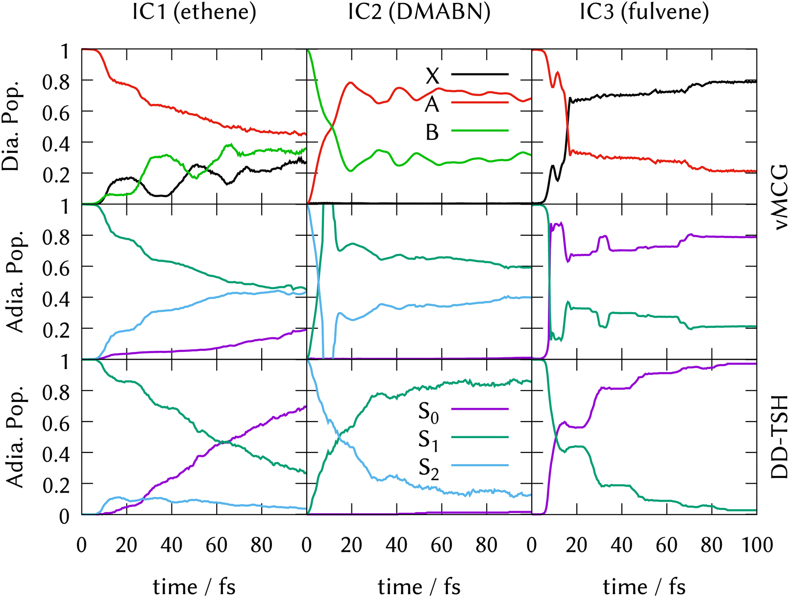
LVC model Hamiltonians were constructed using single-point quantum chemistry calculations of the energies, gradients and derivative couplings for all the states in the manifold at the ground-state optimised geometries, i.e., at the FC point, for all three systems. Along with the ground-state normal modes and frequencies, this provides the parameters for the model as described in Section 3.5. Full dimensional ML-MCTDH dynamics as well as vMCG and TSH simulations were run for 100 fs on these potential energy surfaces. The ML-MCTDH and vMCG simulations ran directly on the model diabatic surfaces, while the TSH trajectories ran on the adiabatic surfaces provided by diagonalising the diabatic potentials. The surfaces used in each case are thus exactly equivalent. The parameters are provided as Quantics operator files in the data sets that are part of the ESI.† The resulting state populations as a function of time are shown in Fig. 1. The top panel shows the converged vMCG and ML-MCTDH diabatic populations, the middle panel the adiabatic populations from the vMCG propagation, and the bottom panel the adiabatic populations averaged over 500 TSH trajectories. The convergence of the method is demonstrated for fulvene in Section S6 of the ESI.†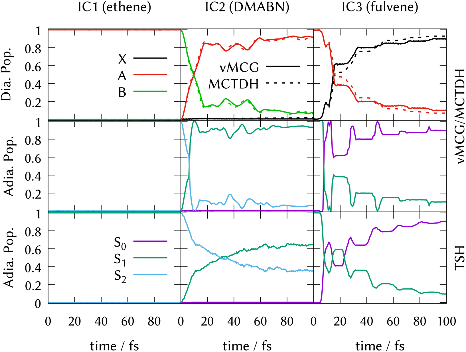 | ||
| Fig. 1 State populations for the three Ibele–Curchod models using LVC Hamiltonians. Top panel: Diabatic populations, vMCG (solid) and MCTDH (dashed). Middle panel: Adiabatic populations, vMCG. Bottom panel: Adiabatic populations, TSH. See text for details. | ||
The state population dynamics are seen to be very different in each case. In ethene (IC1), there is no population transfer. In both DMABN (IC2) and fulvene (IC3) the diabatic population transfer calculated by ML-MCTDH and vMCG is fast and fairly complete, but in the case of IC2 the transfer starts immediately and is almost linear out to 20 fs, after which it plateaus with light oscillations. In IC3, there is a delay before transfer starts. Transfer then takes place in clear steps with a period of around 20 fs.
The adiabatic population transfer from vMCG has a similar character to the diabatic populations. In IC2, the initial linear transfer is complete, followed by a small recurrence and then an oscillating plateau. The TSH results show a similar time-scale, with an immediate start of transfer, but the crossing is slower and not as complete. In IC3, a more complicated adiabatic population dynamics is seen, with crossings and recurrences occurring with a 20 fs period. TSH again provides a similar picture, but the initial population transfers are weaker. The performance of the saddle-point approximation used to obtain the adiabatic populations is shown for IC2 in Section S7 of the ESI.† It leads to an exaggeration of the transfer when passing through the intersection, but gives a reliable approximation when away from the intersection seam.
To classify the types of intersections, the minimum energy point on the LVC model conical intersection seam (MECI) was located using energy minimisation. This used conjugate gradient optimisation of the energy difference between the adiabatic surfaces to reach the seam, followed by energy minimisation of the energy of the upper adiabatic surface, projecting out the gradient difference and non-adiabatic coupling vectors.57 If, during the second step, the system moves away from the seam, the two steps were repeated in an iterative scheme until convergence was reached.
There is no conical intersection in the IC1 LVC model. This is expected as it is known from previous work that the S1/S0 intersection is accessed along the torsional mode.58,59 There is no potential gradient or linear coupling along this mode at the FC point, hence this intersection is not described by the model. The classification of the conical intersections for IC1 will be discussed later.
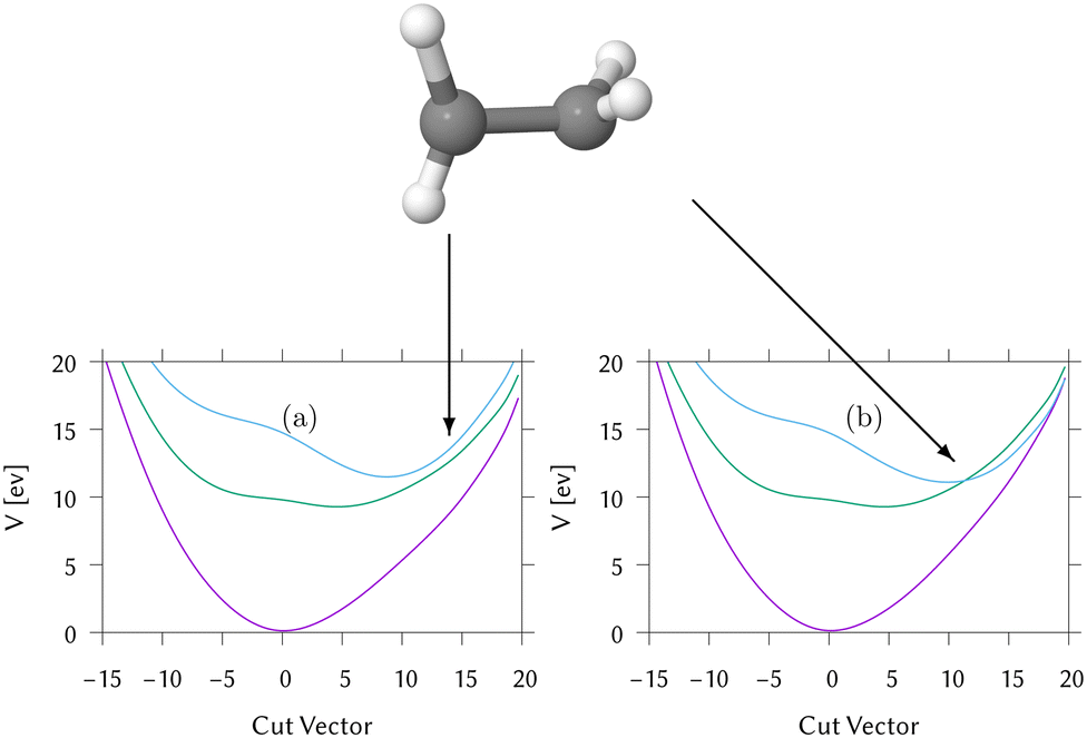
Cuts from the FC point to the MECI for IC2 and IC3 are shown in Fig. 2. These cuts are along normalised vectors made up of a combination of the different vibrations leading to the intersection. The coordinates used are mass-frequency scaled normal modes. In these coordinates, for any normal mode the potential can be written as  and a distance of q = 1 along a normal mode is the extension with a potential energy equal to the zero point energy. The vectors defining the MECIs are given in Section S5 of the ESI.† Both are sloped intersections as the gradients on both surfaces at the intersection point have the same sign. The differences lie in the positions relative to the FC point.
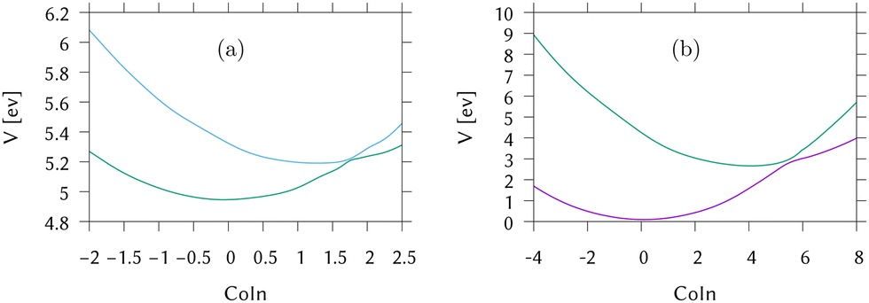 | ||
| Fig. 2 Cuts through the LVC potential energy surfaces for (a) IC2 (DMABN) and (b) IC3 (fulvene) along the vector from FC to MECI. For IC2 the S1/S2 surfaces are shown, while for IC3 the surfaces are for S0/S1. | ||
In IC2, the intersection is at a distance of 1.7 units from the FC point. Given that the width of the initial wavepacket, defined as the standard deviation of the ground-state harmonic oscillator (Gaussian) function, is  the intersection lies under the initial wavepacket and is classified as immediate. This is the reason why population transfer starts immediately in vMCG, whereas in TSH the trajectories still need to move in phase space to reach the intersection, explaining the observed delay. It is also very close in energy, at E = 5.20 eV compared to the energy at the FC point of E = 5.31 eV.
In contrast, the MECI in IC3 is further from the FC region, both in coordinate space and in energy and it is classified simply as a direct intersection. It is at a distance of 5.86 units, so lies well away from initial wavepacket. The energy at the intersection, at E = 2.84 eV, is well below the energy at the FC point of E = 4.16 eV. The IC3 population dynamics can be explained by this classification as the initial delay before transfer begins is the time taken to reach the intersection. The wavepacket then passes through with an efficient adiabatic transfer, due to the speed of the wavepacket on approach. The sloped topography results in an immediate recurrence as the wavepacket is reflected back from the potential wall. The population stays constant after exiting the intersection region, before repeating this passage periodically after oscillating across the well and back. This results in the square-step population dynamics observed.
The geometries of DMABN and fulvene at the MECIs are given in Section S5 of the ESI.† In DMABN it is close to the FC geometry, while for fulvene the ring has contracted and the C![[double bond, length as m-dash]](https://www.rsc.org/images/entities/char_e001.gif) C bond extended.
C bond extended.
4.2 Direct dynamics
As described in the methods above, direct dynamics calculations with the DD-vMCG method were run using the partitioning and basis set of the vMCG calculations, as listed in Table 1. The average energy and standard deviation of the energy are listed too. The norm is kept to 1.0 by renormalising every 1 fs. DD-TSH calculations ran 500 trajectories. The number of accepted trajectories, along with the average energy and energy standard deviation, are also listed in Table 1. Trajectories were rejected if they contained a frustrated hop, or failed to finish. The energy of the DD-vMCG and DD-TSH calculations are different due to an incomplete sampling of the zero-point energy in the DD-TSH runs.State populations as a function of time obtained from the direct dynamics simulations are shown in Fig. 3. The upper two rows show the DD-vMCG diabatic and adiabatic populations from the final calculations on the complete databases. The third row depicts the adiabatic populations obtained from averaging the populations from the independent DD-TSH trajectories.
 | ||
| Fig. 3 State populations for the three Ibele–Curchod models using direct dynamics. Top panel: Diabatic populations, DD-vMCG (solid). Middle panel: Adiabatic populations, DD-vMCG. Bottom panel: Adiabatic populations, TSH. See text for details. | ||
For IC2 (DMABN) and IC3 (fulvene), the behaviour after photo-excitation is qualitatively the same as the LVC results, showing a very quick, near-linear decay of the active state to the S1 in IC2 and in IC3 a delayed fast decay to the S0 followed by periodic recurrences. The final adiabatic population transfer, however, is more complete in the DD-TSH calculations compared to the LVC model, while it is less complete using DD-vMCG. As described above for the LVC populations, the sharp peak in the adiabatic populations of IC2 seen around 10 fs is a result of the saddle-point approximation used to obtain them.
In contrast to the LVC model for IC1 (ethene), direct dynamics predicts a fast decay out of the initially populated state, with 60% being transferred after 100 fs. DD-vMCG shows a diabatic transfer from the A-state to a mixture of the ground X-state and the second excited B-state, which show an out-of-phase oscillatory behaviour. Transforming to the adiabatic picture, this transfer is mostly (40%) to the S2 state and 20% going to the ground state, S0. DD-TSH sees a similar population transfer out of the S1 state, however almost all of the population returns to the ground state, with less than 10% ending up in S2 after 100 fs. This result from DD-TSH compares well to previous work that included only the S0 and S1 adiabatic electronic states.23 The DD-vMCG behaviour, however, is significantly different from this, and reasons for this will be discussed further below.
The final IC1 database for the direct dynamic simulations contained 42907 points, while that for IC2 contained 27294 and for IC3 38354. The structures included in each are shown in Fig. 4. It is clear that ethene and fulvene sample the complete torsional motion, while DMABN remains fairly planar. The structures thus cover the configurations needed to fit with the known behaviour of these molecules in the first 100 fs after photo-activation as the torsional motion is strongly activated in ethene24 and fulvene,31 while DMABN remains planar.33
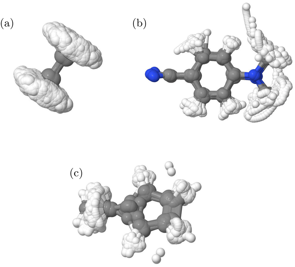 | ||
| Fig. 4 Overlay of structures in the QC databases generated from DD-TSH and DD-vMCG calculations for the (a) IC1, (b) IC2 and (c) IC3 models. | ||
The similarity between the LVC and direct dynamics results for IC2 and IC3 indicate that the potential surfaces are well characterised by the single conical intersection seam of the LVC model. The main addition from the direct dynamics is allowing the molecules to move away from the intersection faster, leading to reduced population transfer due to new pathways being available in the active states. Consequently, the system is prevented from reaching the direct conical intersection present in the LVC model.
This behavior, however, is not shown in TSH dynamics, where the transfer is even more complete using on-the-fly potentials. Since the database used is the same for both dynamics methods, the disparity must be attributed to the intrinsic characteristics of the methods or to the sampling of the initial wavepacket. We assume that the basis functions representing the DD-vMCG wavepacket can coherently find the regions away from the LVC conical intersection, while the independent TSH sampled trajectories do not feel the forces that direct them from the main decay path. Another point for consideration is that in the DD-TSH calculations, the electronic coefficients on non-active states are being damped since they follow the gradient of the active state. However, the potentials show sloped intersections in which the electronic states lie fairly parallel, and therefore the decoherence correction might not be needed, resulting in larger population transfers.
Comparing to Ibele and Curchod,23 we observe that the TSH populations are very similar, which further validates the Quantics implementation of the method. An important difference is observed in IC3, where their TSH population resembles almost perfectly our DD-vMCG population after transforming to the adiabatic picture. This demonstrates how different implementations of the same method may lead to slight variations in the dynamics.
The state population dynamics from the IC1 model show a significant dependence on the method and Hamiltonian used. The DD-TSH population dynamics for IC1 in Fig. 3 agrees with previously published direct dynamics results using methods such as AIMS, stochastic-selection AIMS, multi configurational Ehrenfest, ab initio multiple cloning and previous TSH simulations.15,23,60–63 All of these methods demonstrate a simple fast deactivation from the bright state to the electronic ground state with a time period of 100 fs. In contrast, DD-vMCG predicts a population transfer predominantly from the adiabatic S1 to S2, which is composed of a mixture of diabatic states ![[X with combining tilde]](https://www.rsc.org/images/entities/char_0058_0303.gif) and
and ![[B with combining tilde]](https://www.rsc.org/images/entities/char_0042_0303.gif) (N and V in Mulliken notation35). Further analysis is required to explain this alternative behaviour.
(N and V in Mulliken notation35). Further analysis is required to explain this alternative behaviour.
For this, the MECI in the direct dynamics potential surfaces were located, utilising the same optimisation procedure used to locate the MECI in the LVC models above. These are shown in Fig. 5 and the coordinates for the MECI structures are included in Section S5 of the ESI.† As expected, the approach to the MECI for both IC2 and IC3 are very similar to the those in the LVC model. In IC2 it is an immediate, sloped intersection, while in IC3 it is a direct, sloped intersection.
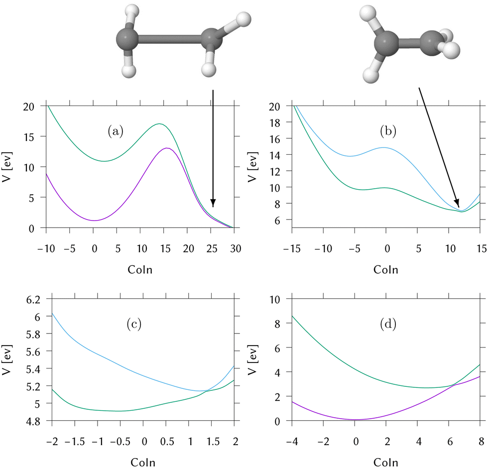 | ||
| Fig. 5 Cut through the direct dynamics potential energy surfaces from the FC point to the MECIs (a) of S0/S1 for IC1 (ethene) (b) of S1/S2 for IC1 (ethene) (c) of S1/S2 for IC2 (DMABN) (d) of S0/S1 for IC3 (fulvene). The x-axis is labelled “CoIn” to emphasise that this data does not represent motion along a specific normal mode. Key: purple = S0, green = S1, blue = S2. | ||
In IC1, conical intersections are found between S1/S0 and S2/S1. Both have an HCCH torsion angle of 90°, and the importance of the torsional motion is seen by the complete lack of population transfer in the simple linear vibronic coupling model calculations in which the torsion has been replaced by a harmonic oscillator. The long range motion allowed by the direct dynamics in contrast to LVC models is thus essential for a good description of this system.
The S2/S1 intersection can be accessed directly from the FC point. However, there is a maxima at the FC point and no gradient directing the excited wavepacket to the MECI. We call this a “second-order direct” intersection. The S1/S0 intersection additionally has significant distortions to the CH2 groups and the C–C bond is extended. By inspection of the surfaces in this region, it is clear that they are not well described by the database. The dynamics did not reach this region and the predicted intersection structure has an RMSD of 0.9 Å from the nearest database point, which is a big distance. As a result the predictions (energetics and structures) are approximations provided by the Shepard scheme which, here, is extrapolating rather than interpolating. However, the ethene S1/S0 conical intersection has been well characterised in the past using multireference methods58,59 and is in this region of configuration space involving torsion and pyramidalisation of the CH2 groups. The high barrier between the FC point and the intersection will clearly hinder direct access of the intersection.
Cuts through the potential surfaces from the FC point of IC1 along the “torsional” mode, q8, the pyramidalisation mode, q2, and the C–C stretch, q5, are shown in Fig. 6. The gradient is along q5 whilst along q2, the surfaces are flat. The S1/S0 intersection can only be reached after activation of modes not activated by the excitation. For this reason the intersection is classified as “indirect”. The direct approach to the S2/S1 intersection is, however, clear in Fig. 6(a), as is the maximum along this mode at the FC point. Fig. 6(b) plots the surfaces along the actual torsion angle, showing the correct symmetry around the intersection seam that is not seen along the normal mode.
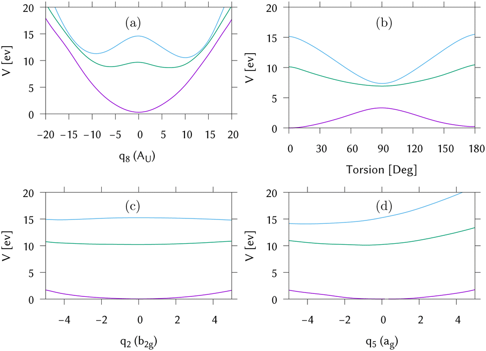 | ||
| Fig. 6 Potential energy cuts through the IC1 (ethene) potential surfaces calculated by direct dynamics away from the Franck–Condon point. (a) Along the “torsional” normal mode, q8. (b) Along the HCCH torsion. (c) Along the pyramidalisation normal mode, q2 and (d) along the C–C stretching vibration, q5. Key: purple = S0, green = S1, blue = S2. | ||
In order to further investigate the different behaviour of IC1, the reduced densities in the three states from the DDvMCG and DD-TSH simulations are plotted in Fig. 7 along the q2 (pyramidalisation) and q8 (torsional) modes. It should be noted that the DD-vMCG densities are in the diabatic picture, while the TSH are in the adiabatic. However, this only alters the state assignments and does not alter the evolution of the density.
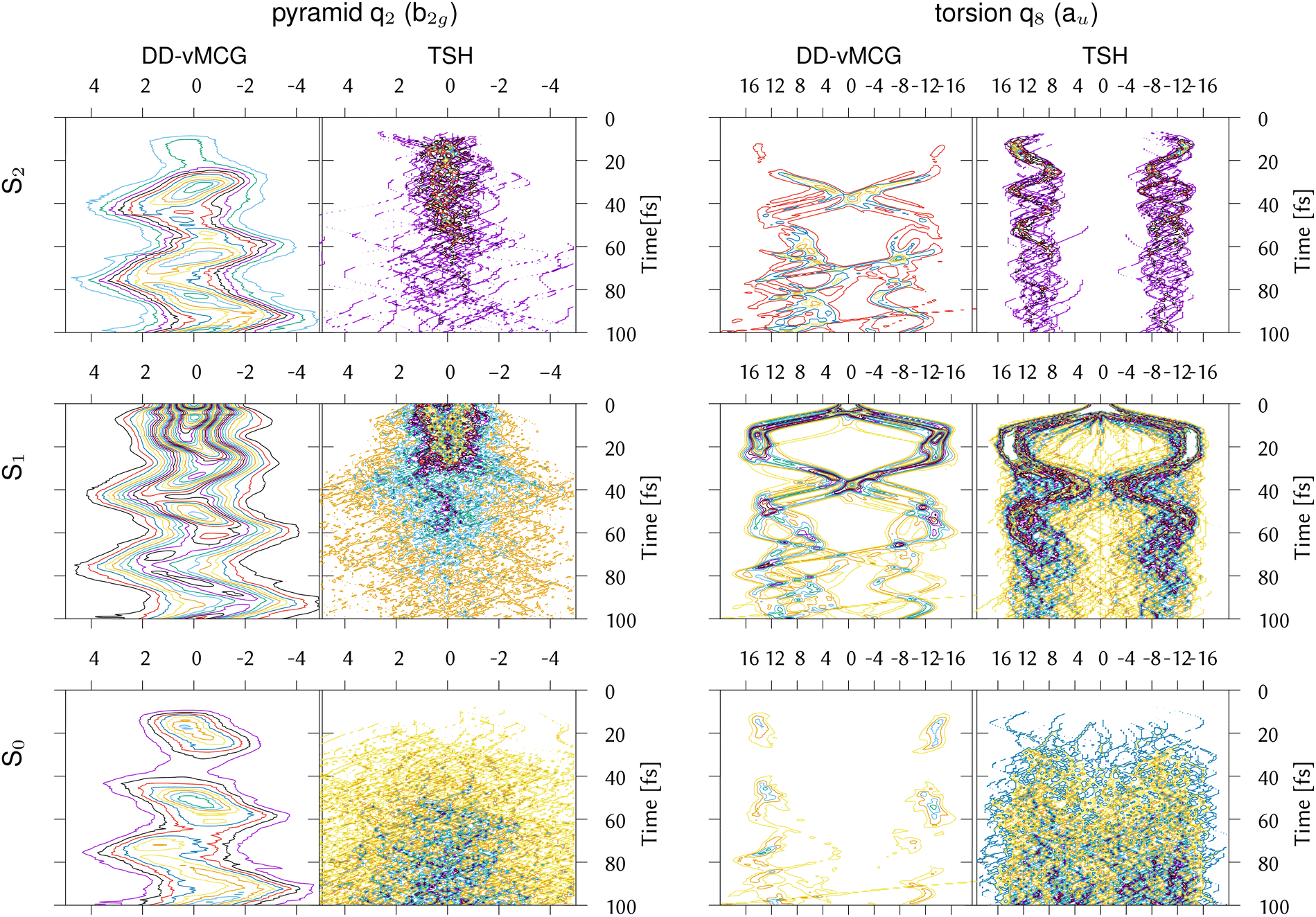 | ||
| Fig. 7 Reduced densities for the IC1 (ethene) model from DD-vMCG calculations with 40/40 GWPs and DD-TSH with 500 trajectories plotted along the CH2 pyramidalisation and torsion normal modes. | ||
Along the torsion, the motion on all states is similar, with a bifurcation of the wavepacket showing the torsional excitation. This is particularly evident for earlier timescales (up to 30 fs) on S1, or Ã, where the wavepacket and trajectories both remain localised. At later times, however, the DD-TSH density spreads over the torsional space. As seen in Fig. 6, a displacement of 11 units along this mode corresponds approximately to a torsion angle of 90°.
The behaviour along the pyramidalisation mode is very different. In the DD-TSH calculations, the pyramidalisation is quickly excited and the density spreads. In the DD-vMCG calculations, however, the density remains compact, staying dense around the equilibrium angle. For this reason the DD-vMCG wavepacket cannot access the S1/S0 conical intersection as easily.
The DD-vMCG result is supported by the work of Viel et al. in ref. 26, who performed full quantum MCTDH simulations on a six dimensional model of ethene using curvilinear coordinates to treat the C–C stretch, torsion, pyramidalisation angles and CH2 bends. The surfaces were calculated at the CASPT2 level and transformed to a diabatic picture. Both diabatic and adiabatic population transfers are similar to the DD-vMCG results presented here: approximately 20% ends in S2 which is a mix of and and minimal population returns to S0. The wavepacket along the pyramidalisation angle also remains compact. Interestingly, recent calculations on 1,1-difluoroethene also show the same discrepancy, with TSH results predicting relaxation from the S1(V) state to the ground state,64 while quantum dynamics simulations indicate that the relaxation goes into energetically close Rydberg states.65
5 Discussion and conclusions
In this paper we set out to establish a set of models, introduced by Ibele and Curchod,23 for testing on-the-fly non-adiabatic dynamics methods. Using these models, we then show the present capabilities of the DD-vMCG algorithm and that the linear vibronic coupling model provides a useful starting point. A new classification of conical intersections has also been introduced to describe the intersections in the three models, highlighting their differences with respect to the dynamics required to reach them.For direct dynamics, a model is defined by the level of quantum chemistry used and the number of states included, along with the starting point. Here, the original Ibele–Curchod models are extended by including the S2 state in the model based on ethene (IC1), and by a different functional used for the model IC2 based on DMABN. These changes were made for practical reasons: the upper state is found to be important for the IC1 dynamics and the functional was found in a previous study to provide a better description of DMABN.
For all three models, TSH is found to provide similar results to previous work, with fast population transfer from the initial state to the state below. The results from DD-vMCG are similar for IC2 and IC3, but significantly different for IC1. For a comparison of the methods, it must be kept in mind that, while the theoretical basis of vMCG means it is able to reproduce the full quantum result on the LVC models, there are two approximations introduced in the direct dynamics implementation. The first of the these is the diabatisation of the potential surfaces, and the second is the use of a local harmonic approximation in calculating integrals involving the potentials. While these have to be shown to work well on small systems, there is no guarantee how well they perform on large, complex systems. TSH, of course, is an approximate method with classical nuclei and is hence not guaranteed to be able to reproduce a quantum simulation. Its performance also depends on the exact algorithm as well as the implementation.
In the Quantics code, the potential surfaces for direct dynamics are provided by interpolating points (energies, gradients and Hessians) stored in a database. The points are collected during the simulations, but can then be re-used in subsequent calculations. This has the advantage not only of providing a global description of the potentials, which can be used in later analysis, but also has the potential to significantly reduce the number of quantum chemistry calculations required. If 500 surface hopping trajectories are run with a 0.5 fs time step for 100 fs, this requires 100000 calculations. In the calculations presented here, the databases created contain between 20000 and 40000 points, representing a significant reduction of effort for the DD-vMCG simulations. These interpolated surfaces can also be used for TSH calculations and more trajectories can be run at minimal cost.
Future work will explore further savings of effort by reducing the number of points required. It is clear that IC2 and IC3 are well described by LVC Hamiltonians, which requires only a single point. It is apparent that a substantial proportion of computational effort is being wasted due to redundant points present in the database, hence better algorithms to calculate new points only when required must be implemented. A possible way forward is the statistical measures developed by the Collins group in relation to the Grow methodology for PES production.66,67
The first point in the database provides a quadratic vibronic coupling model Hamiltonian, expanding the surfaces around the FC point to second order with the coupling to first order. Running dynamics on this QVC model is a useful exercise at the start of a study as it can also be used with the grid-based MCTDH wavepacket method to provide an exact solution as an initial benchmark. Here we used simpler LVC Hamiltonians that ignored the excited-state second-order terms, but the principle is the same. The populations in the dynamics show that, in fact, the IC2 and IC3 models are very well described by the LVC models.
In order to describe the conical intersections responsible for the population transfer dynamics, the MECIs were found in the LVC models and the full surfaces obtained from the direct dynamics. For IC2 and IC3, the point found in the LVC model and full database are very similar. However, they differ in the two models due to the distance the MECI is from the FC point. In IC2 the intersection is close to the FC point and lies under the initial wavepacket, resulting in the population transfer starting immediately. In IC3, the intersection seam is reached directly from the FC point, but requires some time to reach it. As the MECI in both IC2 and IC3 has a sloped topography, we classify them as “immediate sloped” and “direct sloped”, respectively. The different topographies leave a signature in the state population dynamics.
The behaviour of IC1 (ethene) is quite different from the other two models. Firstly, the LVC model does not contain a conical intersection. The S2/S1 seam is reached by the HCCH torsion changing from 0° to ±90° and is far from the harmonic diabatic potential of the LVC model. In the direct dynamics simulations where this torsional motion is allowed, however, there is a disagreement between the DD-vMCG and DD-TSH results. In the DD-vMCG calculations, little population (20% after 100 fs) is transferred to the ground state, while in the DD-TSH simulations 70% of the population is transferred in 70 fs, in line with earlier studies. This difference poses a challenge.
On the direct dynamics potentials, the S2/S1 MECI can be directly accessed from the FC point, but there is no gradient in this direction. Instead the surfaces exhibit a steep saddle point at the FC point and the wavepacket bifurcates after excitation to S1. This leads to fast crossing from S1 to S2, and we classify this intersection as “second-order direct”. From the geometry of ethene at the S1/S0 MECI, additional activation of the CH2 pyramidalisation mode is needed. There is no gradient along this mode, and as a result the intersection is classified as “indirect” as it cannot be reached directly from the FC point, but requires energy to flow into this mode for efficient crossing. This mode is weakly activated in the DD-vMCG simulations, and may account for the difference.
An answer to the difference is potentially given by first looking in detail at the state populations in Fig. 3. It can be seen that both the DD-vMCG and DD-TSH calculations initially populate the S2 state. In the DD-TSH calculations, however, this population is quickly transferred to S0, whereas in DD-vMCG this does not happen. To connect this to the dynamics, the one-dimensional densities along the pyramidalisation (q2) and torsional (q8) normal modes are shown in Fig. 7 from the DD-vMCG and DD-TSH simulations. Analysis of the DD-TSH results show that most hops to the ground state occur after torsional rotation, but with little pyramidalisation, showing that the system is able to find accessible portions of the seam without much energy flowing into this mode, i.e. away from the MECI. Where the hops take place in the space of the torsional and pyramidalisation normal modes is shown in the ESI,† Fig. S10.
To get an idea of the potential surfaces being accessed, a “representative hopping structure” was made by averaging over the 537 geometries where hops took place. A cut from the Franck–Condon point to this structure through both the adiabatic and diabatic potentials is shown in Fig. 8. The structure has a torsion angle near to 180° and a light pyramidalisation. The coordinates for this structure are in Table S17 in the ESI.† Approach to this structure on the intially populated S1 state is barrierless and the S2/S1 diabatic surfaces cross. The S2 diabatic state then goes on to meet S1 showing that all three states are close in energy in this region. Looking at the densities in Fig. 7, in the DD-TSH calculations, after crossing to the S2 state the system stays at the torsionally deformed geometry, with a torsion angle close to 90°. This is where the three surfaces are close in energy so hops down to S0 can occur, and on the ground-state surface the trajectories quickly spread out so the population remains in this state. In contrast, in the DD-vMCG simulation, after crossing to S2, the torsion angle quickly rotates back to 0° and the population remains trapped in that state.
 | ||
| Fig. 8 Cut through the (a) adiabatic and (b) diabatic potential surfaces of IC1 from the Franck–Condon point (at a distance of 0) to a representative geometry where hopping takes place (at a distance of 13.0). The geometry is shown above the cuts. | ||
A second point to note is that in the DD-vMCG simulations the density remains more compact along q2, than in the DD-TSH simulations. Thus if pyramidalisation helps to provide efficient transfer to S0 the coherence in the vMCG wavepacket would hinder this. It is noted that the density along q2 should remain symmetric due to the symmetry of the potentials, and this is not the case in the DD-vMCG simulations, which exhibit a light osciallatory motion. This is an artefact due to the numerical integration of the vMCG equations of motion, but is too small to affect averaged quantities such as state populations. To support this, the trajectories along this coordinate from the centres of the DD-vMCG GWP basis functions are plotted in Fig. S12 in the ESI,† along with those from the DD-TSH simulation. The loss of symmetry after 10 fs is seen, as well as the compact region of space covered by the DD-vMCG wavepacket compared to that covered by the surface hopping trajectories.
Can we say which of these results is correct? It is possible that the diabatisation scheme used in DD-vMCG is not able to correctly reproduce the complicated intersection seams. However, on a visual inspection of the potential surface topography, and supported by reduced dimensional wavepacket calculations,26 it seems that the DD-vMCG result makes sense. Unfortunately, a definitive answer cannot be provided by experiment due to the simplicity of the model. Experiments on ethene indicate that the maximum of the absorption band to the V state is located at 162 nm, which is 7.65 eV.35 The 3s Rydberg state is beneath it at the FC point and can be probed at 6.3 eV.68 The V state in our CAS(2,2) model locates the V state at 10.2 eV, over 2.5 eV above the experimental value and very close to the ionisation threshold. The latest time-resolved experiments68,69 seem to support a direct transfer from the bright V state to the ground state, whereas earlier results70 uphold the idea of populating intermediate Rydberg states to access the ground state, similar to our previous results in difluoroethylene.64 Both experiments agree in the initial movement of the molecule upon excitation, consisting of a mixture of stretching and torsion and state that the wavepacket quickly moves away from the FC excitation with a timescale of 18 fs. Keeping in mind the limitations of the electronic structure, we support the rapid torsional and stretching motion, driving the molecule away from the FC point in the sub-20 fs timescale. What we observe, however, is a mixture from V and Z states, supported by the experiments of ref. 70 which cannot distinguish states V and Z, due to the degeneracy of orbitals at torsion angles of 90°.
High level complete wavepacket dynamics results are also not available. As mentioned above, the 6-mode, 3-state model of Viel et al.26 supports the low population transfer to S0. However, this was at a different level of theory and did not include all modes which may restrict access to the intersection seam. The most complete calculations on ethene are an MRCI 17-state full dimensional study by Jornet-Somoza et al.28 These calculations demonstrate that after excitation to the V state, the population becomes trapped in a Rydberg state and does not return to the ground state. The presence of the Rydberg states, however, makes it challenging to compare to the present, simple, 3-state model.
In conclusion, vMCG is able to reproduce the results of grid-based dynamics on analytical LVC Hamiltonians based on the Ibele–Curchod models. The direct dynamics version, DD-vMCG, provides potential surfaces and quantum dynamics on the full systems. Differences with surface hopping trajectories on the same surfaces, however, point to the need for further work testing the approximations in the way DD-vMCG is implemented, as well as developing ways to make the comparison of methods in different representations more rigorous.
One possibility for the introduction of comparability would be performing a diabatisation of the TSH populations. While it is a known problem to perform globally consistent diabatisations, a number of diabatisation methods have been explored and implemented.21,61,71–73 Future work will include the implementation and testing of a method for the diabatisation of the TSH populations, as well as the development of appropriate analysis tools.
The three Ibele–Curchod models thus provide an excellent set of tests for direct non-adiabatic dynamics. These models cover three different types of dynamics, mediated by four different types of conical intersection seams. IC3 is the most straightforward, while in IC2 the challenge is the size of the system. The most challenging is IC1 where competition between intersections is present and future work is still required to analyse the results from IC1 to make it a benchmark in the true sense. Despite this, the utilization of these models will establish an initial basis for the evaluation of direct dynamics methods, akin to the way the original Tully models are employed to test non-adiabatic dynamics methods.
Conflicts of interest
There are no conflicts to declare.Acknowledgements
SG acknowledges NextGenerationEU funds (María Zambrano Grant for the attraction of international talent). ES and GW acknowledge funding from the EPSRC as part of the Programme Grant EP/V026690/1. All authors thank CECAM and the Lorentz Centre, Leiden, for organising workshops which provoked the need for benchmarks in non-adiabatic dynamics simulations.Notes and references
- J. C. Tully, J. Chem. Phys., 1990, 93, 1061–1071 CrossRef CAS.
- M. F. Herman, J. Chem. Phys., 1984, 81, 754–763 CrossRef CAS.
- M. H. Beck, A. Jäckle, G. A. Worth and H.-D. Meyer, Phys. Rep., 2000, 324, 1–105 CrossRef CAS.
- R. Kosloff, J. Phys. Chem., 1988, 92, 2087–2100 CrossRef CAS.
- F. Agostini and B. F. E. Curchod, Wiley Interdiscip. Rev.: Comput. Mol. Sci., 2019, 9, e1417 Search PubMed.
- M. Bonfanti, G. A. Worth and I. Burghardt, Multi-Configuration Time-Dependent Hartree Methods: From Quantum to Semiclassical and Quantum-Classical, John Wiley & Sons, Ltd, 2020, ch. 12, pp. 383–411 Search PubMed.
- I. S. Y. Wang and M. Karplus, J. Am. Chem. Soc., 1973, 95, 8160–8164 CrossRef CAS.
- J. A. Pople, D. P. Santry and G. A. Segal, J. Chem. Phys., 1965, 43, S129–S135 CrossRef CAS.
- J. A. Pople and G. A. Segal, J. Chem. Phys., 1965, 43, S136–S151 CrossRef CAS.
- C. Leforestier, J. Chem. Phys., 1978, 68, 4406–4410 CrossRef CAS.
- W. J. Hehre, W. A. Lathan, R. Ditchfield, M. D. Newton and J. A. Pople, Gaussian 70 (Quantum Chemistry Program Exchange, Program No. 237), 1970 Search PubMed.
- T. Helgaker, E. Uggerud and H. J. A. Jensen, Chem. Phys. Lett., 1990, 173, 145–150 CrossRef CAS.
- T. Vreven, F. Bernardi, M. Garavelli, M. Olivucci, M. A. Robb and H. B. Schlegel, J. Am. Chem. Soc., 1997, 119, 12687–12688 CrossRef CAS.
- IBM, A Guide to the IBM System/370 Model 168, IBM, 3rd edn, 1975 Search PubMed.
- M. Ben-Nun, J. Quenneville and T. J. Martínez, J. Phys. Chem. A, 2000, 104, 5161–5175 CrossRef CAS.
- B. Lasorne, M. A. Robb and G. A. Worth, Phys. Chem. Chem. Phys., 2007, 9, 3210–3227 RSC.
- K. Saita and D. V. Shalashilin, J. Chem. Phys., 2012, 137, 22A506–22A508 CrossRef PubMed.
- M. Barbatti, G. Granucci, M. Persico, M. Ruckenbauer, M. Vazdar, M. Eckert-Maksić and H. Lischka, J. Photochem. Photobiol., A, 2007, 190, 228–240 CrossRef CAS.
- M. Richter, P. Marquetand, J. González-Vázquez, I. Sola and L. González, J. Chem. Theory Comput., 2011, 7, 1253–1258 CrossRef CAS PubMed.
- G. A. Worth and M. A. Robb, Adv. Chem. Phys., 2002, 124, 355–432 CrossRef CAS.
- R. Crespo-Otero and M. Barbatti, Chem. Rev., 2018, 118, 7026–7068 CrossRef CAS PubMed.
- B. F. E. Curchod and T. Martínez, Chem. Rev., 2018, 118, 3305–3336 CrossRef CAS PubMed.
- L. M. Ibele and B. F. E. Curchod, Phys. Chem. Chem. Phys., 2020, 22, 15183–15196 RSC.
- J. Quenneville, M. Ben-Nun and T. J. Martínez, J. Phys. Chem. A, 2000, 104, 5161–5175 Search PubMed.
- K. K. Baeck and T. J. Martínez, Chem. Phys. Lett., 2003, 375, 299–308 CrossRef CAS.
- A. Viel, R. P. Krawczyk, U. Manthe and W. Domcke, J. Chem. Phys., 2004, 120, 11000–11010 CrossRef CAS PubMed.
- M. R. Brill, F. Gatti, D. Lauvergnat and H.-D. Meyer, Chem. Phys., 2007, 338, 186–199 CrossRef CAS.
- J. Jornet-Somoza, B. Lasorne, M. A. Robb, H.-D. Meyer, D. Lauvergnat and F. Gatti, J. Chem. Phys., 2012, 137, 84304 CrossRef PubMed.
- M. J. Bearpark, F. Bernardi, M. Olivucci, M. A. Robb and B. R. Smith, J. Am. Chem. Soc., 1996, 118, 5254–5260 CrossRef CAS.
- F. Sicilia, M. J. Bearpark, L. Blancafort and M. A. Robb, Theor. Chem. Acc., 2007, 118, 241–251 Search PubMed.
- L. Blancafort, F. Gatti and H.-D. Meyer, J. Chem. Phys., 2011, 135, 134303 CrossRef PubMed.
- B. F. E. Curchod, A. Sisto and T. J. Martínez, J. Phys. Chem. A, 2017, 121, 265–276 CrossRef CAS PubMed.
- S. Gómez, E. N. Soysal and G. A. Worth, Molecules, 2021, 26, 1–20 Search PubMed.
- G. J. Atchity, S. S. Xantheas and K. Ruedenberg, J. Chem. Phys., 1991, 95, 1862–1876 CrossRef.
- A. J. Merer and R. S. Mulliken, Chem. Rev., 1969, 69, 639–656 CrossRef CAS.
- Y. Shao, Z. Gan, E. Epifanovsky, A. T. Gilbert, M. Wormit, J. Kussmann, A. W. Lange, A. Behn, J. Deng, X. Feng, D. Ghosh, M. Goldey, P. R. Horn, L. D. Jacobson, I. Kaliman, R. Z. Khaliullin, T. Kuś, A. Landau, J. Liu, E. I. Proynov, Y. M. Rhee, R. M. Richard, M. A. Rohrdanz, R. P. Steele, E. J. Sundstrom, H. L. W. III, P. M. Zimmerman, D. Zuev, B. Albrecht, E. Alguire, B. Austin, G. J. O. Beran, Y. A. Bernard, E. Berquist, K. Brandhorst, K. B. Bravaya, S. T. Brown, D. Casanova, C.-M. Chang, Y. Chen, S. H. Chien, K. D. Closser, D. L. Crittenden, M. Diedenhofen, R. A. D. Jr., H. Do, A. D. Dutoi, R. G. Edgar, S. Fatehi, L. Fusti-Molnar, A. Ghysels, A. Golubeva-Zadorozhnaya, J. Gomes, M. W. Hanson-Heine, P. H. Harbach, A. W. Hauser, E. G. Hohenstein, Z. C. Holden, T.-C. Jagau, H. Ji, B. Kaduk, K. Khistyaev, J. Kim, J. Kim, R. A. King, P. Klunzinger, D. Kosenkov, T. Kowalczyk, C. M. Krauter, K. U. Lao, A. D. Laurent, K. V. Lawler, S. V. Levchenko, C. Y. Lin, F. Liu, E. Livshits, R. C. Lochan, A. Luenser, P. Manohar, S. F. Manzer, S.-P. Mao, N. Mardirossian, A. V. Marenich, S. A. Maurer, N. J. Mayhall, E. Neuscamman, C. M. Oana, R. Olivares-Amaya, D. P. ONeill, J. A. Parkhill, T. M. Perrine, R. Peverati, A. Prociuk, D. R. Rehn, E. Rosta, N. J. Russ, S. M. Sharada, S. Sharma, D. W. Small, A. Sodt, T. Stein, D. Stück, Y.-C. Su, A. J. Thom, T. Tsuchimochi, V. Vanovschi, L. Vogt, O. Vydrov, T. Wang, M. A. Watson, J. Wenzel, A. White, C. F. Williams, J. Yang, S. Yeganeh, S. R. Yost, Z.-Q. You, I. Y. Zhang, X. Zhang, Y. Zhao, B. R. Brooks, G. K. Chan, D. M. Chipman, C. J. Cramer, W. A. G. III, M. S. Gordon, W. J. Hehre, A. Klamt, H. F. S. III, M. W. Schmidt, C. D. Sherrill, D. G. Truhlar, A. Warshel, X. Xu, A. Aspuru-Guzik, R. Baer, A. T. Bell, N. A. Besley, J.-D. Chai, A. Dreuw, B. D. Dunietz, T. R. Furlani, S. R. Gwaltney, C.-P. Hsu, Y. Jung, J. Kong, D. S. Lambrecht, W. Liang, C. Ochsenfeld, V. A. Rassolov, L. V. Slipchenko, J. E. Subotnik, T. V. Voorhis, J. M. Herbert, A. I. Krylov, P. M. Gill and M. Head-Gordon, Mol. Phys., 2015, 113, 184–215 CrossRef CAS.
- H.-J. Werner, P. J. Knowles, G. Knizia, F. R. Manby and M. Schütz, Wiley Interdiscip. Rev.: Comput. Mol. Sci., 2012, 2, 242–253 CAS.
- H.-J. Werner, P. J. Knowles, F. R. Manby, J. A. Black, K. Doll, A. Heßelmann, D. Kats, A. Köhn, T. Korona, D. A. Kreplin, Q. Ma, I. Miller, F. Thomas, A. Mitrushchenkov, K. A. Peterson, I. Polyak, G. Rauhut and M. Sibaev, J. Chem. Phys., 2020, 152, 144107 CrossRef CAS PubMed.
- H.-J. Werner, P. J. Knowles, P. Celani, W. Györffy, A. Hesselmann, D. Kats, G. Knizia, A. Köhn, T. Korona, D. Kreplin, R. Lindh, Q. Ma, F. R. Manby, A. Mitrushenkov, G. Rauhut, M. Schütz, K. R. Shamasundar, T. B. Adler, R. D. Amos, S. J. Bennie, A. Bernhardsson, A. Berning, J. A. Black, P. J. Bygrave, R. Cimiraglia, D. L. Cooper, D. Coughtrie, M. J. O. Deegan, A. J. Dobbyn, K. Doll, M. Dornbach, F. Eckert, S. Erfort, E. Goll, C. Hampel, G. Hetzer, J. G. Hill, M. Hodges, T. Hrenar, G. Jansen, C. Köppl, C. Kollmar, S. J. R. Lee, Y. Liu, A. W. Lloyd, R. A. Mata, A. J. May, B. Mussard, S. J. McNicholas, W. Meyer, T. F. Miller III, M. E. Mura, A. Nicklass, D. P. O'Neill, P. Palmieri, D. Peng, K. A. Peterson, K. Pflüger, R. Pitzer, I. Polyak, M. Reiher, J. O. Richardson, J. B. Robinson, B. Schröder, M. Schwilk, T. Shiozaki, M. Sibaev, H. Stoll, A. J. Stone, R. Tarroni, T. Thorsteinsson, J. Toulouse, M. Wang, M. Welborn and B. Ziegler, MOLPRO, version 2020, a package of ab initio programs, https://www.molpro.net Search PubMed.
- G. A. Worth, Comput. Phys. Commun., 2020, 248, 107040 CrossRef.
- G. A. Worth, K. Giri, G. W. Richings, I. Burghardt, M. H. Beck, A. Jäckle and H.-D. Meyer, Quantics package, Version 2.0, 2022 Search PubMed.
- G. W. Richings and G. A. Worth, J. Phys. Chem. A, 2015, 119, 12457–12470 CrossRef CAS PubMed.
- G. Christopoulou, A. Freibert and G. A. Worth, J. Chem. Phys., 2021, 154, 124127 CrossRef CAS PubMed.
- W. Xie, M. Sapunar, N. Došlić, M. Sala and W. Domcke, J. Chem. Phys., 2019, 150, 154119 CrossRef PubMed.
- J. Coonjobeeharry, K. E. Spinlove, C. Sanz Sanz, M. Sapunar, N. Došlić and G. A. Worth, Philos. Trans. R. Soc., A, 2022, 380, 20200386 CrossRef CAS PubMed.
- J. C. Light, I. P. Hamilton and J. V. Lill, J. Chem. Phys., 1985, 82, 1400–1409 CrossRef CAS.
- H.-D. Meyer, F. Gatti and G. A. Worth, Multidimensional Quantum Dynamics: MCTDH Theory and Applications, Wiley-VCH, Weinheim, Germany, 2009 Search PubMed.
- O. Vendrell and H.-D. Meyer, J. Chem. Phys., 2011, 134, 44135 CrossRef PubMed.
- U. Manthe, J. Chem. Phys., 2008, 128, 164116 CrossRef PubMed.
- H. Wang and M. Thoss, J. Chem. Phys., 2003, 119, 1289–1299 CrossRef CAS.
- E. J. Heller, J. Chem. Phys., 1981, 75, 2923 CrossRef CAS.
- G. A. Worth and B. Lasorne, Gaussian Wave Packets and the DD-vMCG Approach, John Wiley & Sons, Ltd, 2020, ch. 13, pp. 413–433 Search PubMed.
- I. Burghardt, H.-D. Meyer and L. S. Cederbaum, J. Chem. Phys., 1999, 111, 2927–2938 CrossRef CAS.
- G. Granucci and M. Persico, J. Chem. Phys., 2007, 126, 134114 CrossRef PubMed.
- H. Köppel, W. Domcke and L. S. Cederbaum, Adv. Chem. Phys., 1984, 57, 59–246 CrossRef.
- G. A. Worth and L. S. Cederbaum, Ann. Rev. Phys. Chem., 2004, 55, 127–158 CrossRef CAS PubMed.
- M. J. Bearpark, M. A. Robb and H. B. Schlegel, Chem. Phys. Lett., 1994, 223, 269 CrossRef CAS.
- M. Ben-Nun and T. J. Martínez, Chem. Phys., 2000, 259, 237–248 CrossRef CAS.
- H. Tao, B. G. Levine and T. J. Martínez, J. Phys. Chem. A, 2009, 113, 13656–13662 CrossRef CAS PubMed.
- D. V. Makhov, W. J. Glover, T. J. Martinez and D. V. Shalashilin, J. Chem. Phys., 2014, 141, 054110 CrossRef PubMed.
- W. Zhou, A. Mandal and P. Huo, J. Phys. Chem. Lett., 2019, 10, 7062–7070 CrossRef CAS PubMed.
- B. F. E. Curchod, W. J. Glover and T. J. Martínez, J. Phys. Chem. A, 2020, 124, 6133–6143 CrossRef CAS PubMed.
- G. Granucci, M. Persico and A. Toniolo, J. Chem. Phys., 2001, 114, 10608–10615 CrossRef CAS.
- S. Gómez, L. M. Ibele and L. González, Phys. Chem. Chem. Phys., 2019, 21, 4871–4878 RSC.
- S. Gómez, N. K. Singer, L. González and G. A. Worth, Can. J. Chem, 2023, 101, 745–757 CrossRef.
- M. A. Collins, Theor. Chem. Acc., 2002, 108, 313–324 Search PubMed.
- T. J. Frankcombe, M. A. Collins and G. A. Worth, Chem. Phys. Lett., 2010, 489, 242–247 CrossRef CAS.
- T. Kobayashi, T. Horio and T. Suzuki, J. Phys. Chem. A, 2015, 119, 9518–9523 CrossRef CAS PubMed.
- S. Karashima, A. Humeniuk, W. J. Glover and T. Suzuki, J. Phys. Chem. A, 2022, 126, 3873–3879 CrossRef CAS PubMed.
- K. Kosma, S. A. Trushin, W. Fuss and W. E. Schmid, J. Phys. Chem. A, 2008, 112, 7514–7529 CrossRef CAS PubMed.
- B. R. Landry, M. J. Falk and J. E. Subotnik, J. Chem. Phys., 2013, 139, 211101 CrossRef PubMed.
- C. S. Pradhan and A. Jain, J. Chem. Theory Comput., 2022, 18, 4615–4626 CrossRef CAS PubMed.
- Y. Shu, Z. Varga, S. Kanchanakungwankul, L. Zhang and D. G. Truhlar, J. Phys. Chem. A, 2022, 126, 992–1018 CrossRef CAS PubMed.
Footnote |
| † Electronic Supplementary Information (ESI) available. See DOI: https://doi.org/10.1039/d3cp03964a |
| This journal is © the Owner Societies 2024 |