In situ dissolved polypropylene prediction by Raman and ATR-IR spectroscopy for its recycling

Abstract

Monitoring the dissolution of polyolefins using online spectroscopy analysis is addressed in this work, with the aim of optimizing plastic recycling processes. Two in situ spectroscopic methods are used to predict the dissolved polymer content: Raman spectroscopy and attenuated total reflectance infrared spectroscopy. Commercially available polypropylenes are considered. Different solvents are selected based on their affinity with polypropylene. Partial least squares regression is employed to identify models predicting the polymer concentration for each solvent from the online spectra. Raman spectroscopy was found to give a better prediction. It was therefore used to study different parameters influencing the dissolution process, such as solvent type, temperature and polymer form.

---

1. Introduction

Since the 50s, approximately 9 billion tons of plastics have been produced worldwide due to their importance in several domains, and this production is expected to triple by 2050.¹ However, the rise of production leads to the generation of more waste, of different types. Large pieces of plastics spilled in nature may be ingested by animals, and micro- and nanoplastics pollute water and plants causing a big impact on our health and the environment.² Moreover, due to the 260 megatons of plastic waste produced annually,³ the weight of emitted CO₂ during plastic incineration is three times more than the incinerated plastic.^4,5 Thus, CO₂ emission by plastic production and incineration may exceed 50 gigatons within 30 years which would correspond to almost 10% of the global carbon emission. Nevertheless, plastic materials are essential in our daily life. To maintain their production while reducing their environmental impact, we need to reduce the way we consume, rethink the way we reuse and optimize the way we recycle them.

While it's true that plastic pollution in oceans, on our planet, and in the air is a significant issue, it arises from usage, collection, and the behavior of populations. Recycling alone won't solve the problem of plastic dispersion. Recycling is, in fact, one factor among many: finding outlets for waste gives value to these discarded materials. It's essential to activate all these levers to bring about meaningful change. Different recycling ways are employed, including mechanical recycling and chemical recycling. Among chemical recycling techniques, the dissolution/purification technique is the most promising because it offers the possibility to recover a virgin resin free of all additives, like pigments, and the polymer can possibly be reused in different ways other than the initial application.⁴ For example, xylene as solvent and isopropanol as anti-solvent were used for the separation of low density polyethylene from alumina in post-consumer cartons, where 99.5% of the alumina-polyethylene laminates were recovered.⁶ More recently, a polyolefin recycling process was developed based on polymer dissolution, optional washing and adsorption, and extraction that ensures efficient purification of the resins.⁷ In this work, we are interested in developing an online method for monitoring this process.

Given the diversity of additives, developing a dissolution recycling process to purify the polymer from all the charges is a challenging task. Therefore, monitoring the dissolution and precipitation steps is essential for process optimization. Although ex situ analyses of virgin polymer resins and plastic additives are widely exploited, these techniques require complex sampling (handling pressure, temperature, multiphase medium) and may present a risk of non-representativeness especially in big non uniform vessels or when the samples evolve quickly. To ensure process security, enhance productivity, and maintain control of the properties of the final product, it is crucial to incorporate online monitoring.

Several spectroscopic analysis techniques are usually used to analyze polymer products offline and online. For instance, water content has been monitored by in situ near infrared (NIR) spectroscopy in a continuous conversion reactor.⁸ Infrared spectroscopy with Fourier transform (FT-IR) has been employed to compare polyethylene samples before and after a dissolution process, to study the impact of the process on the microstructure of the polymer (i.e. degradation issues) and optimize the process.^9,10In situ Raman spectroscopy has been used to monitor polypropylene (PP) degradation after multiple extrusion cycles.¹¹ NIR and mid-infrared (MIR) spectroscopies are also commonly used for waste sorting,^12,13 and directing the waste towards mechanical or chemical recycling processes.

Although there is a considerable interest in spectroscopic analyses of plastic matrices, monitoring the dissolution and precipitation of polyolefins using spectroscopic analysis has not been addressed in the literature. This work will explore this topic with the aim of monitoring and optimizing polymer recycling processes. Two in situ spectroscopic methods have been compared for the monitoring of the dissolved polymer content: Raman and attenuated total reflectance (ATR)-infrared spectroscopies. Commercial PP samples were investigated. Different solvents were selected based on their affinity with PP, using the Hansen solubility parameter. The developed models are then used to study the different parameters influencing dissolution, such as the nature of the solvent and temperature.

2. Experimental section

2.1. Polymers and solvent

A commercial PP in pellets form of the mm order, has been chosen and characterized by different analytical techniques. It exhibits a weight average molar mass (M_w) of 170 kg mol⁻¹, a crystallinity of 54% and a melting temperature of 166.5 °C. The PP has been reshaped in a powder form of the order of 100 μm, it was obtained by cryo-milling of the pellets, where all the polymer properties remain the same (type of polymer, molar mass, branching, crystallinity, etc.) and only the form changes. The reagent grades solvents xylene, n-decane, decahydronaphthalene (decalin) and 1,2,4 trichlorobenzene (TCB) were purchased from Sigma-Aldrich and were used without further purification.

2.2. Instrument

2.2.1. Raman. A Kaiser Optical Systems RXN2 Raman spectrometer equipped with a 785 nm laser of 400 mW power was used with an immersion probe of 12 mm in diameter. The acquisition conditions were as follow: 5 seconds of integration time, and 10 scans are averaged to give 1 spectrum each minute. The wavelength region ranges from 100 cm⁻¹ to 3425 cm⁻¹.

2.2.2. ATR-IR. IR spectra (1800 to 800 cm⁻¹) were collected with a Nicolet™ iS50 FTIR Spectrometer equipped with an attenuated total reflection (ATR) immersion probe (Diamond) of 12 mm in diameter. Each IR spectrum corresponds to an accumulation of 128 scans with a resolution of 8 cm⁻¹ giving one spectrum every 2 minutes.

2.3. Dissolution vessel

The dissolution equipment consists of a 500 mL glass jacketed vessel, heated by an oil bath. The vessel was equipped with a cooled condenser to condense the boiling solvent. The medium was mixed by a 4-blades propeller. The two 12 mm diameter spectral probes and a temperature probe were inserted into the medium. An argon flow was put in the air of the vessel to avoid penetration of oxygen and polymer degradation during the dissolution. By this way, spectral changes were only due to polymer dissolution. For each experiment, the required amount of solvent was first introduced in the vessel. Then, the temperature was increased to the desired value using the heating bath. Once the temperature set point was reached, polypropylene was added in 300 mL of solvent (in pellet forms or in powder form after cryo-milling of the pellets) at a known concentration. After dissolution, the solution is cooled to room temperature, polypropylene is precipitated and washed using methanol, then dried at 100 °C before reuse.

2.4. Solvent selection

The selection of the solvents was based on the solubility parameter similarity with polypropylene.¹⁴ The Hansen solubility parameters (δ_d, δ_p, δ_h) of polypropylene¹⁵ and various solvents¹⁶ are listed in Table S1† where δ_d (in MPa^1/2) is the solubility parameter related to dispersive energy forces, δ_p is related to permanent dipole forces and δ_h is related to hydrogen-bonding forces.¹⁷ Based on these parameters, a Hansen solubility sphere could be defined to predict the polymer solubility in the investigated solvents.¹⁸ Solvents located within this polymer solubility sphere, as illustrated Fig. S1,† are theoretically capable of dissolving the polymer (i.e. compatible) while the solvents outside the sphere are not compatible, although the polymer molar mass, branching or crystallinity also have an effect on the solubility. Besides the solubility efficiency, solvent selection was constrained by other factors. Solvents from different chemical families were aimed, to cover a wide applicability of the monitoring methodology, namely a linear alkane, a cyclic alkane, an alkylated aromatic, and a halogenated aromatic. Additionally, solvents with a high boiling point were targeted to enable the dissolution temperature to be increased while operating at atmospheric pressure. From Table S1, Fig. S1,† and the above-mentioned constraints, the selected solvents for polypropylene dissolution are xylene, decahydronaphthalene (decalin), decane and 1,2,4 TCB. The properties of these solvents are indicated in Table S2.†

2.5. Sampling and reference method

Samples were collected at different intervals using a glass pipet previously heated with a heating band to avoid precipitation of polypropylene during the sampling. The pipet was equipped with a filter to avoid taking polymer particles.

The gravimetric method was used as the reference method for measuring the polymer fraction in the solvent. In this method, a uniform part of the sample was put in a vial. The mass of the sampling vial was measured (with a precision of ±0.1 mg) before and after solvent evaporation. The solvent was evaporated by drying under vacuum at 110 °C and 10⁴ Pa for 8 hours, followed by an additional drying at atmospheric pressure in an oven at 100 °C for 24–48 h. Error bars of the reference method were estimated based on 10 samples at a fixed concentration of 10% w/v, leading to a standard deviation of 0.7% w/v. Note that at low polymer concentrations, the sampling was easier due to the lower viscosity of the medium, so the measurements are reproducible. But, as the fraction of polymer increases, the viscosity increases, making the sampling more difficult, and therefore the bias is expected to become higher.

2.6. Data analysis

Partial Least Squares Regression (PLSR), a commonly employed multivariate calibration technique, was used for quantification based on spectral data. This algorithm conducts a regression analysis to correlate input variables (spectra) known as the X block, along with the target property of interest (polymer content), referred to as the Y block. The data is projected onto a reduced-dimensional space called the latent variable space. During the calibration phase, it is crucial to select the optimal number of latent variables (LVs) and eliminate any outlier samples to ensure reliable and valid results during the validation process.¹⁹ The implementation was performed using the PLS Toolbox v9.1 and MATLAB. Different preprocessing methods were evaluated. For the Raman spectra, the best performance models were obtained when using the first derivative Savitzky–Golay with a second polynomial order smoothing (SavGol[15,2,1]). Some regions were removed because of a strong response of the neon: 407–422 cm⁻¹, 1354–1341 cm⁻¹, 1535–1546 cm⁻¹ and 2885–2871 cm⁻¹. Other regions were removed because they contain no essential information: 100–200 cm⁻¹, 1600–2600 cm⁻¹ and 3200–3425 cm⁻¹. Concerning the ATR-IR spectra, only an SVG smoothing (SavGol[15,0]) was applied, as other pretreatments were not efficient and added noise. The left part of the spectra, from 1450 cm⁻¹ to 1800 cm⁻¹, was removed because this region provides no information about the polymer and is impacted by temperature, thus biasing the model.

2.6.1. External parameter orthogonalization (EPO). The spectral data encompass information that is influenced by both the factor of interest and external factors. By employing orthogonal projection onto the subspace with EPO preprocessing,²⁰ the original spectra can be projected in a manner that effectively eliminates the influence of external factors. EPO pretreatment was carried out in the calibration set to eliminate the temperature effect by acquiring spectra in a wide temperature range.

2.6.2. Selection of latent variables (LVs). A PLS model with EPO preprocessing was developed to predict the concentration of dissolved polypropylene in each solvent separately, from the Raman or ATR-IR spectra based on 20 different concentrations and different temperatures. The acquired spectra were split into a calibration set and a validation set by removing 5 concentrations (3% w/v, 7% w/v, 11% w/v, 14% w/v and 18% w/v) entirely from the calibration set (i.e., all temperatures) to the prediction set. Contiguous blocks cross-validation was realized with 10 data splits. The indicators of model quality, used to select the LVs, are the root-mean-square errors of calibration (RMSEC), cross-validation (RMSECV) and prediction (RMSEP):where y_i and ŷ_i are respectively the measured and predicted polypropylene concentrations of the sample i, and n and k are the number of samples in the calibration and validation set respectively. The optimal number of LVs is obtained for the lowest values of RMSEC and RMSECV to ensure robustness and at the same time avoid overfitting.

2.6.3. Calibration data. The initial step in developing reliable calibration equations consists of a careful selection of representative samples. The calibration samples were chosen to cover the entire range of operating conditions of interest (in this case, concentration) and to accommodate for unforeseen process variations not explicitly captured by the reference calibration method, such as temperature variations and fluctuations of additives concentrations. 20 different samples with concentrations varying from 1% w/v to 20% w/v (of fully dissolved PP) were used for calibration. These are typical concentrations encountered in recycling processes, between the beginning of polymer dissolution until full dissolution.^21,22

For each concentration, the temperature was varied, with a ramp of 1.25 °C min⁻¹, ranging from 135 °C to 160 °C, so ensuring no PP precipitation or degradation. The spectra were acquired at 20 different temperatures for Raman spectroscopy and 10 different temperatures for ATR-IR spectroscopy. We ensured visually and through the reference method (gravimetry) that the PP is completely dissolved in the temperature range for each solvent by considering the worst case (i.e. dissolving the maximal fraction of 20% w/v of PP at the lowest temperature 135 °C). For all the calibration set, a dissolution time of 30 min at a stirring speed of 200 rpm was applied to reach complete dissolution. This procedure was repeated for the 4 selected solvents. Thus, we have 400 Raman spectra and 200 IR spectra for each calibration set in each solvent. Fig. S2† shows the flow diagram decision for the construction of the calibration set.

2.7. Design of experiment

A design of experiments was proposed to systematically vary several operating conditions (Table 1). The primary focus is on changing the solvent, temperature, and the form of polymer (pellets or powder obtained by cryo-milling of the pellets). The agitation rate was fixed at 200 rpm. The concentration notation %w/v refers to a ratio between the mass of PP to the volume of solvent (e.g. 10% w/v means 100 g of PP in 1 L of solvent). This allows the dissolution kinetics in different solvents to be compared.

Table 1 Operating conditions of the different dissolution experiments of PP

Run	Solvent	Concentration (%w/v)	Temperature (°C)	Form
1	Xylene	10	130	Pellets
2	Decane	10	130	Pellets
3	TCB	10	130	Pellets
4	Decalin	10	130	Pellets
5	Decane	10	150	Pellets
6	Decane	10	170	Pellets
7	Decalin	10	150	Pellets
8	Decalin	10	170	Pellets
9	TCB	10	150	Pellets
10	TCB	10	170	Pellets
11	Xylene	2	130	Pellets
12	Xylene	4	130	Pellets
13	Xylene	20	130	Pellets
14	Xylene	10	130	Powder
15	TCB	10	130	Powder

---

3. Results and discussion

3.1. Spectral analysis

3.1.1. Band assignment of the Raman and ATR-IR spectra. Fig. 1 shows the intensity spectra during the dissolution of PP for run 3 in 1,2,4 TCB using Raman spectroscopy. The spectra are colored according to time (from blue to yellow). We can observe the appearance and increase of the PP bands with time. The Raman bands of PP are well identified in the literature.²³ The 808 cm⁻¹ and 974 cm⁻¹ bands are due to the –CH₃ rocking vibration, the bands at 1326 cm⁻¹ and 1436 cm⁻¹ can be attributed to the –CH₂ bending vibration, and the other bands around 2900 cm⁻¹ are related to the C–C backbone stretching vibration.

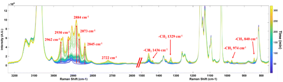Fig. 1 Bands assignment of the raw Raman spectra of PP in TCB at 130 °C (run 3) in the 700–1500 cm⁻¹ and 2500–3200 cm⁻¹ regions.

FT-IR spectroscopy has the particularity to be an efficient and relatively simple method for the characterization and identification of polymers. Fig. 2 shows the in situ IR spectra of the calibration set involving all the PP contents at the different temperatures for each content. The main IR bands of PP are the –CH₂ scissoring vibration at 1377 cm⁻¹, the two bands of the –CH₃ rocking vibration at 997 cm⁻¹ and 973 cm⁻¹ and the rocking vibration of the CH₂ bond at 840 cm⁻¹.²⁴

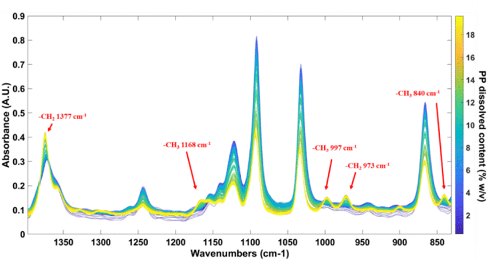Fig. 2 Bands assignment of the raw ATR-IR spectra of PP in TCB calibration set in the 830 cm⁻¹ to 1400 cm⁻¹ region.

3.1.2. Model development. Temperature correction has been performed using EPO preprocessing. Fig. S3 and S4† show the principal component analysis (PCA) scores for the calibration set in decalin, before and after pre-treatment, by Raman and ATR-IR respectively. The EPO preprocessing is more efficient on the Raman calibration set than the ATR-IR calibration set where the temperature effect has not been completely removed. Furthermore, random variation is observed on the ATR-IR calibration set, which can mainly be explained by the low resolution and limited spectral range of the ATR-IR spectra.

The number of LVs was determined using the model quality indicators. Fig. 3 shows the evolution of RMSEC and RMSECV as a function of the number of LVs for the ATR-IR and Raman models of PP in the solvent TCB. The errors first decrease, then stabilize after few LVs of about 3–4.

Fig. 3 Root mean square error of calibration and cross-validation according to the number of latent variables using the PLS model of the concentration of PP in TCB in (a) ATR-IR and (b) Raman.

The loadings of the PLS model were carefully examined to avoid considering too noisy and undesirable LVs. Fig. S5† shows the loadings of the three first LVs of the ATR-IR and Raman models in TCB. All of them contain chemical band effects of PP and the level of noise is low. For instance, the band with the higher impact in the first two ATR-IR loadings, representing together 99.84% of the variability, is the 1377 cm⁻¹ band of the –CH₂ scissoring vibration. The models are therefore based on the PP bands and can predict the concentration of PP during the dissolution. For the TCB model using ATR-IR, we chose 3 LVs to ensure a low RMSECV and avoid overfitting.

In the Raman model, 3 LVs also were enough to explain 99% of the variability. Fig. S5† shows that the LVs are governed by the 3 PP zones: the C–C stretching (2900 cm⁻¹), –CH₂ bending (1326–1436 cm⁻¹) and –CH₃ rocking (808–974 cm⁻¹). This low number of latent variables could be selected in the different solvents, ensuring an optimized relationship between the PP content and the spectra.

3.1.3. Examining outliers. The outliers were identified and removed by studying the residuals in predicting the polymer concentration, the Q residuals reduced, and the Hotelling T². They represent, respectively, the gap between the measured and predicted concentration, the disparity between a sample and its projection onto the LVs retained in the model and the atypicality of the samples relative to the model. Plotting the Q residual versus Hotelling T² allows the outliers to be identified when samples remain outside the thresholds of both parameters.²⁵

Fig. S6(a) and S7(a)† shows the residuals plots for ATR-IR and Raman models in TCB respectively, where the red dashed lines represent the acceptable limit of deviation by taking a 95% confidence interval. These figures illustrate a uniform distribution of the values resulting in a homogeneity of variance and thus providing evidence of the absence of model overfitting and a good prediction across the entire evaluation range of the studied property. The distribution is broader for the ATR-IR model than for the Raman model, implying a higher error. This can be explained mainly by the low-resolution and the higher temperature dependence of infrared spectra. The limited spectral range imposed by the in situ probe is also a constraint because only few PP bands are available to predict the polymer content.

To determine if the predicted sample, which falls outside the acceptable limit, can be classified as an outlier, a graphical analysis was conducted by combining the Q residuals and Hotelling T² statistical analyses in Fig. S6(b) and S7(b)† for ATR-IR and Raman models respectively. For the ATR-IR model, six samples (four of the calibration test and two of the test set) were outside the acceptable limit (exceeding thresholds of both the Q and T² test).²⁶ However, these samples were not identified as outliers because no significant difference was observed on the spectra or during the acquisition. The inadequate prediction of these samples can be attributed to the limit of quantification of the technique since they correspond to low concentrations. For the Raman model, 4 samples of the calibration set had an atypical behavior but removing them did not impact the model performances and they were therefore not considered as outliers.

3.1.4. Model performances. For all the solvents, Raman models show better performances, as it can be seen from the parity plots of the measured and the predicted concentrations by the Raman and ATR-IR spectra in the different solvents in Fig. 4. The 95% interval is obtained as twice the RMSECV.²⁷

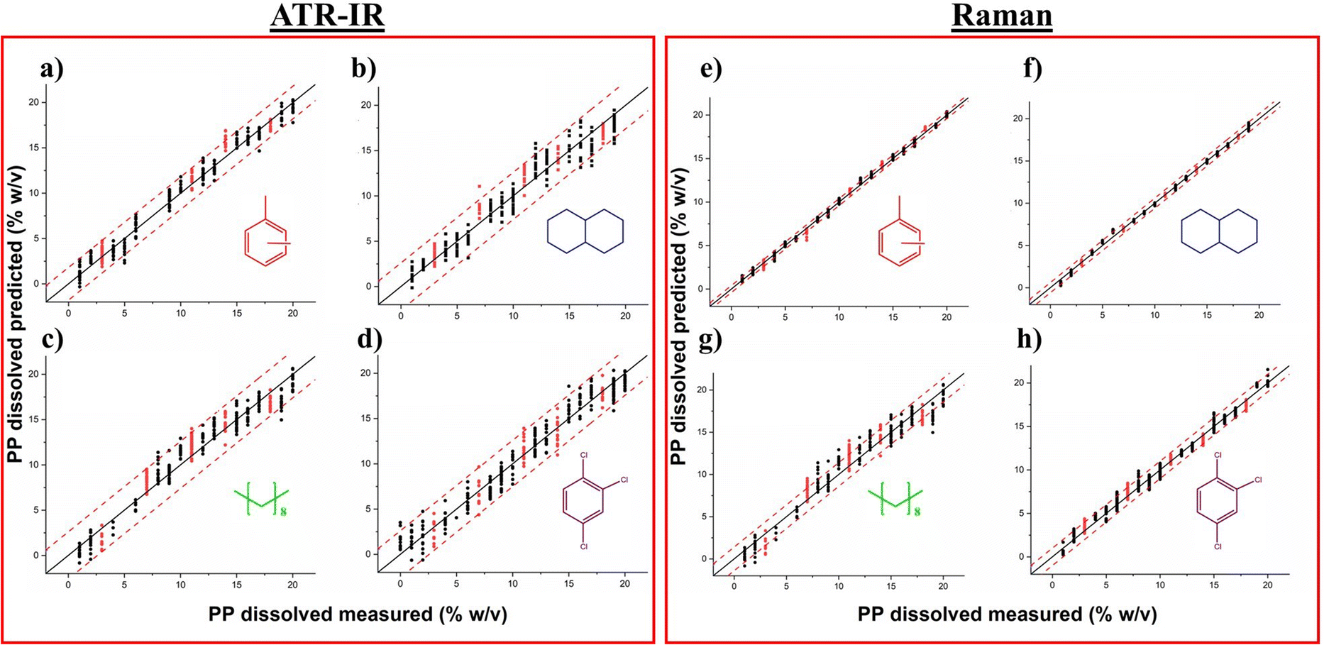Fig. 4 Parity plots of the concentration of dissolved PP using ATR-IR spectroscopy in (a) xylene (b) decalin (c) decane and (d) TCB and using Raman spectroscopy in (e) xylene (f) decalin (g) decane and (h) TCB. The black dots represent the calibration set, the red dots represent the validation set, the black full line represents the 1 : 1 parity line and the red dashed lines represents the 95% confidence interval.

Table 2 summarizes the comparison of the model performance of the ATR-IR and Raman models in each solvent. The use of a PLS regression enables the estimation of the polymer concentration in solution based on spectroscopic information, yielding an acceptable error of less than 1 %w/v for Raman spectroscopy and around 1 %w/v for ATR-IR spectroscopy. Additionally, the squared correlation coefficient (R²) ensures that the developed models provide reliable predictions over the whole range of concentrations evaluated in this study.

Table 2 Raman and ATR-IR model performance in each solvent

	Xylene		n-decane		Decalin		TCB
	Raman	IR	Raman	IR	Raman	IR	Raman	IR
LVs	3	4	3	2	2	3	3	3
RMSEC	0.23	0.85	0.77	1.23	0.29	1.28	0.54	1.06
RMSECV	0.24	0.88	0.76	1.26	0.29	1.32	0.55	1.14
RMSEP	0.35	1.08	1.07	1.38	0.14	1.31	0.59	0.87
R ^2 of C	0.998	0.978	0.979	0.948	0.997	0.949	0.989	0.968
R ^2 of CV	0.998	0.976	0.979	0.945	0.997	0.945	0.989	0.972
R ^2 of P	0.998	0.975	0.957	0.919	0.999	0.955	0.986	0.961

---

3.2. Validation and application of the models

The different models have been separately applied for in situ monitoring of PP dissolution under different conditions. For each experiment, around 15 samples have been collected. Fig. 5 compares the prediction of the polymer content during run 2 (using decane), run 3 (TCB) and run 8 (decalin). Both spectroscopic methods can predict the polymer content as confirmed by the reference method. However, Raman spectroscopy gives a more reliable prediction than ATR-IR. Therefore, for the rest of the study, only the Raman predictions will be used to study the effect of the operating conditions on the dissolution process.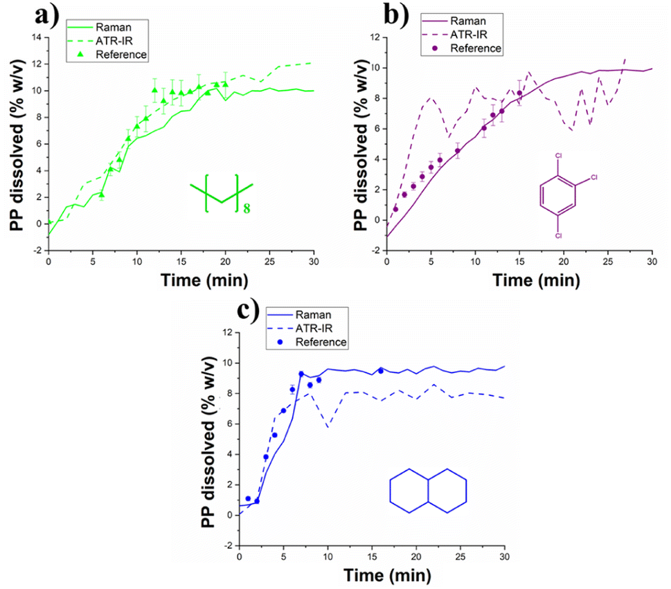

Fig. 5 Comparison of the ATR-IR and Raman prediction of the polymer content in (a) decane (b) TCB and (c) decalin.

3.2.1. Effect of the nature of the solvent on the dissolution kinetic. PP was dissolved in the four solvents at 130 °C and a concentration of 10 %w/v (see runs 1 to 4 in Table 1). Fig. S8† shows the predicted polymer concentration for these runs, where only the solvent was changed. The Raman PLS model predicted the final concentration with ±1% accuracy and provided an acceptable prediction of the dissolution kinetics as confirmed by gravimetry. All solvents totally dissolve the considered amount of PP at the end, but they seem to have different dissolution kinetics. Different works showed that semi-crystalline polymers have a specific behavior during their dissolution.^28,29 Initially, the solvent permeates in the amorphous phase of the polymer, leading to the formation of a swollen layer at the surface. This swollen layer gradually infiltrates the polymer core. On one hand, polymer chains present on the gel layer surface come apart and disperse into the solvent bulk region. On the other hand, the crystallites undergo decrystallization upon contact with the solvent. The polymer gradually transitions to a fully amorphous state, with the polymer chains diffusing into the bulk of the solvent. In both Raman and IR spectroscopy, the spectra will be mainly sensitive to the amount of polymer that is well dissolved in the solvent. The predictions of the concentration of dissolved PP in the different solvents are superposed in Fig. 6.

Fig. 6 Prediction of the dissolved polymer content in the different solvents by Raman spectroscopy (runs from 1 to 4 at 130 °C with an agitation of 200 rpm).

The fastest solvent to dissolve the polymer seems to be xylene, followed by decalin, decane and finally TCB. This means that PP shows a higher dissolution rate in aromatics and naphthenic than in n-alkanes and halogenic compounds. This can be explained partly by the affinity of PP with these solvents. The general solubility parameter δ can be calculated based on the values given Table S1:†

δ² = δ_h² + δ_p² + δ_d² (3)

Eqn (3) gives a solubility parameter for PP of 18.2, for xylene of 18.1, for decalin of 17.6, for decane of 16, and for TCB of 20.9. The closest solvent to PP and thus, the one showing the highest affinity, is xylene, then decalin, decane and TCB. Also, the solvent molar volume may affect the dissolution rate. Indeed, the rate at which solvent molecules permeate, depends on their molar volume.^30,31 Xylene has the smallest molar volume (Table S2†), and a good affinity with PP (Fig. S1†), leading to a high dissolution rate. Conversely, decane has a particularly large molar volume but still has a higher dissolution rate than TCB, since both solvents are approximately at the same distance from PP (Fig. S1†) and the higher flexibility of linear n-alkanes allows them to more easily permeate into the polymer. It is expected that lower carbon number n-alkanes may have a higher dissolution rate since the molecules diffuse faster. Such experiments could not be performed in the available set-up due to the low boiling point of small n-alkanes which would require working in a closed pressurized vessel. This effect was noted by Blackadder et al.³² who observed a higher dissolution rate of PP in n-octane than in n-decane.

3.2.2. Effect of the polymer concentration on the dissolution time. Increasing the concentration of the solvent can enhance the dissolution of semi-crystalline polymers at a certain temperature, over a specific range. In our study, complete dissolution is ensured at all the studied concentrations at 130 °C as can be seen from Fig. 7. However, the dissolution with 2% w/v polymer is faster than with 10% w/v and 20% w/v. Indeed, a higher concentration of the solvent increases the driving force for solvation and helps to overcome the cohesive forces within the polymer structure.³³ It ensures effective swelling of the polymer matrix, which improves the diffusion rate of the solvent. It also helps to disperse the dissolved polymer chains from the surface of particles. Other thermodynamic properties might be influenced by the polymer concentration in the solvent, such as vapor pressure and osmotic pressure, that can impact the dissolution.³⁴

Fig. 7 Prediction of the dissolved polymer content in xylene at various concentrations corresponding to runs 1, 12 and 13 at 130 °C.

3.2.3. Effect of the temperature on the dissolution rate. As discussed above, the dissolution of semi-crystalline polymers is more complex than amorphous polymers. Semicrystalline polymers exhibit a similar behavior as amorphous polymers once the crucial step of solvent-induced polymer decrystallization takes place.³⁵ To deconstruct this thermodynamically favorable organization of polymer chains, a large amount of energy needs to be brought to the system at the endothermic “decrystallization” step. Also increasing the temperature increases the rates of diffusion of solvent and polymer chains.

Ghasemi et al.³⁵ pointed out that, following the attainment of maximum swelling of the amorphous phase, the dissolution rate is predominantly governed by the rate at which polymer chains disentangle. The disentanglement rate is governed by the diffusion of solvent molecules in the boundary layer of polymer as well as the diffusion of polymer chains towards the solvent phase. An increase in the temperature will result in a higher diffusion, so a higher dissolution rate.

Fig. 8 shows the predictions of runs 2 to 10 with a polymer concentration of 10% w/v, in decalin, decane and TCB at 3 different temperatures: 130 °C, 150 °C and 170 °C. A regular increase in the dissolution rate of decalin is observed when increasing the temperature (Fig. 8a). In the case of decane (Fig. 8b), an increase of the dissolution rate is observed with temperature, with a less significant change between 150 °C and 170 °C, indicating a possible limit of the effect of temperature on the penetration of the solvent molecules and disentanglement of PP chains into the solvent. For TCB, (Fig. 8c), the dissolution time has no specific change between 130 °C and 150 °C, but when the dissolution temperature is equal to 170 °C, we observe a clear increase in the dissolution rate. In all cases a good prediction by Raman is observed.

Fig. 8 Prediction of the dissolved polymer content as for different temperature in (a) decalin, (b) decane and (c) TCB.

3.2.4. Effect of the polymer form (powder or pellets) on the dissolution rate. The form of the polymer introduced into the dissolution vessel is a critical parameter from an industrial point of view. The plastic wastes are usually reshaped before dissolution (in an extruder, granulator, etc.). It is therefore essential to be able to estimate the dissolution kinetics as a function of the form and size of the polymer objects to be dissolved. Fig. 9 compares the dissolution rates between PP powder and pellets. The polymer form has a large effect on the dissolution rate in both solvents xylene and TCB. In the case of the powder form, the contact surface between the polymer and the solvent is improved compared to pellets form. Therefore, much more solvent molecules can interact with the polymer at the interfaces, resulting in almost instantaneous dissolution, especially in xylene.

Fig. 9 Prediction of the dissolved polymer content as a function of the form of polymer in (a) xylene and (b) TCB.

4. Conclusions

This work centers on the estimation of the dissolved polymer content by Raman and ATR-IR spectroscopy. The results indicate the feasibility of this estimation, with a better predictive performance by Raman spectroscopy. Raman spectroscopy, coupled with PLS modeling and EPO preprocessing to eliminate the temperature effect on the spectra was therefore employed for online monitoring of the dissolution rate of PP under different operating conditions (solvent type and concentration, temperature and polymer form). The dissolution kinetics of polymers in solvents are dictated by several parameters: the solvent affinity with the polymer, the characteristics of the solvent molecules (such as their size and flexibility) as well as the polymer properties (ex. molar mass, crystallinity, density). Some operating conditions, such as the temperature and concentrations also influence the dissolution rate. The methodology allowed to have a first look on the parameters that influence the dissolution rate in the used solvents. The diffusivity of solvent and PP molecules increased when increasing the temperature, resulting in a higher dissolution rate. Increasing the contact surface of the polymer objects also led to an increased dissolution rate. In all cases, Raman spectroscopy has proven to be an efficient, fast, and reliable analytical method to monitor in situ and in real time PP dissolution. This model can be useful for the prediction of the dissolved polymer content during polymer waste recycling, it can be used for the selection of efficient solvents in recycling processes, to study the dissolution kinetics, or can be extended to monitor other properties such as polymer degradation.

Author contributions

S. Ferchichi: conceptualization, data curation, model development, writing – original draft. N. Sheibat-Othman: conceptualization, writing – review and editing, supervision. M. Rey-Bayle: conceptualization, model development, supervision. O. Boyron: model development. C. Bonnin: design of experiment conception. S. Norsic: dissolution vessel conception. V. Monteil: conceptualization, writing – review and editing, supervision. All authors have given approval to the final version of the manuscript.

Conflicts of interest

The authors declare no conflict of interest.

Acknowledgements

The authors would like to thank IFP Energies Nouvelles for funding.

References

1. H.-W. Schiffer, WEC energy policy scenarios to 2050, Energy Policy, 2008, 36, 2464–2470.
2. J. Gigault, A. ter Halle, M. Baudrimont, P.-Y. Pascal, F. Gauffre, T.-L. Phi, H. El Hadri, B. Grassl and S. Reynaud, Current opinion: What is a nanoplastic?, Environ. Pollut., 2018, 235, 1030–1034.
3. T. Hundertmark, M. Mayer, C. S. Mcnally, J. Theo and C. Witte, How Plastics Waste Recycling Could Transform the Chemical Industry, McKinsey & Company, 2018.
4. I. Vollmer, M. J. F. Jenks, M. C. P. Roelands, R. J. White, T. van Harmelen, P. de Wild, G. P. van der Laan, F. Meirer, J. T. F. Keurentjes and B. M. Weckhuysen, Beyond Mechanical Recycling: Giving New Life to Plastic Waste, Angew. Chem., Int. Ed., 2020, 59, 15402–15423.
5. A. Vlasopoulos, J. Malinauskaite, A. Żabnieńska-Góra and H. Jouhara, Life cycle assessment of plastic waste and energy recovery, Energy, 2023, 277, 127576.
6. I. Georgiopoulou, G. D. Pappa, S. N. Vouyiouka and K. Magoulas, Recycling of post-consumer multilayer Tetra Pak® packaging with the Selective Dissolution-Precipitation process, Resour., Conserv. Recycl., 2021, 165, 105268.
7. W. Weiss, D. L. Le Cocq, M. Sibeaud and A. H. Ahmadi-Motlagh, Method for treating waste plastics by polymer dissolution and adsorption purification, AU Pat., AU2021403394, 2023.
8. H. W. Ward and F. E. Sistare, On-line determination and control of the water content in a continuous conversion reactor using NIR spectroscopy, Anal. Chim. Acta, 2007, 595, 319–322.
9. A. J. Hadi, G. F. Najmuldeen and I. Ahmed, Polyolefins Waste Materials Reconditioning Using Dissolution/Reprecipitation Method, APCBEE Proc., 2012, 3, 281–286.
10. A. J. Hadi, G. F. Najmuldeen and K. B. Yusoh, Dissolution/reprecipitation technique for waste polyolefin recycling using new pure and blend organic solvents, J. Polym. Eng., 2013, 33, 471–481.
11. X. Guo, Z. Lin, Y. Wang, Z. He, M. Wang and G. Jin, In-Line Monitoring the Degradation of Polypropylene under Multiple Extrusions Based on Raman Spectroscopy, Polymers, 2019, 11, 1698.
12. S. Serranti, A. Gargiulo and G. Bonifazi, Classification of polyolefins from building and construction waste using NIR hyperspectral imaging system, Resour., Conserv. Recycl., 2012, 61, 52–58.
13. C. Signoret, A.-S. Caro-Bretelle, J.-M. Lopez-Cuesta, P. Ienny and D. Perrin, MIR spectral characterization of plastic to enable discrimination in an industrial recycling context: II. Specific case of polyolefins, Waste Manage., 2019, 98, 160–172.
14. C. M. Hansen, The Universality of the Solubility Parameter, Prod. Res. Dev., 1969, 8, 2–11.
15. C. M. Hansen, Hansen Solubility Parameters. A User's Handbook, Taylor et Francis, Boca Raton, 2007.
16. C. M. Hansen, Three dimensional solubility parameter and solvent diffusion coefficient importance in surface coating formulation, Dr thesis, Danish Technical Press, 1967.
17. I. C. Sanchez and R. H. Lacombe, Statistical Thermodynamics of Polymer Solutions, Macromolecules, 1978, 11, 1145–1156.
18. R. C. Gorre and T. P. Tumolva, Solvent and non-solvent selection for the chemical recycling of waste Polyethylene (PE) and Polypropylene (PP) metallized film packaging materials, IOP Conf. Ser. Earth Environ. Sci., 2020, 463, 12070.
19. P. Geladi and B. R. Kowalski, Partial least-squares regression: a tutorial, Anal. Chim. Acta, 1986, 185, 1–17.
20. J.-M. Roger, F. Chauchard and V. Bellon-Maurel, EPO–PLS external parameter orthogonalisation of PLS application to temperature-independent measurement of sugar content of intact fruits, Chemom. Intell. Lab. Syst., 2003, 66, 191–204.
21. A. Chaudhary, M. Dave and D. S. Upadhyay, Value-added products from waste plastics using dissolution technique, Mater. Today: Proc., 2022, 57, 1730–1737.
22. G. Pappa, C. Boukouvalas, C. Giannaris, N. Ntaras, V. Zografos, K. Magoulas, A. Lygeros and D. Tassios, The selective dissolution/precipitation technique for polymer recycling: a pilot unit application, Resour., Conserv. Recycl., 2001, 34, 33–44.
23. E. Andreassen, in Polypropylene, Springer, Dordrecht, 1999, pp. 320–328.
24. M. R. Jung, F. D. Horgen, S. V. Orski, V. Rodriguez C, K. L. Beers, G. H. Balazs, T. T. Jones, T. M. Work, K. C. Brignac, S.-J. Royer, K. D. Hyrenbach, B. A. Jensen and J. M. Lynch, Validation of ATR FT-IR to identify polymers of plastic marine debris, including those ingested by marine organisms, Mar. Pollut. Bull., 2018, 127, 704–716.
25. L. S. Magwaza, S. I. Messo Naidoo, S. M. Laurie, M. D. Laing and H. Shimelis, Development of NIRS models for rapid quantification of protein content in sweetpotato [Ipomoea batatas (L.) LAM.], LWT–Food Sci. Technol., 2016, 72, 63–70.
26. C. Stein, The Admissibility of Hotelling's $T^2$-Test, Ann. Math. Stat., 1956, 27, 616–623.
27. D. G. Altman and J. M. Bland, Standard deviations and standard errors, BMJ, 2005, 331, 903.
28. S. K. Mallapragada and N. A. Peppas, Crystal unfolding and chain disentanglement during semicrystalline polymer dissolution, AIChE J., 1997, 43, 870–876.
29. B. A. Miller-Chou and J. L. Koenig, A review of polymer dissolution, Prog. Polym. Sci., 2003, 28, 1223–1270.
30. J. S. Papanu, D. W. Hess, D. S. Soane and A. T. Bell, Dissolution of Thin Poly(methyl methacrylate) Films in Ketones, Binary Ketone/Alcohol Mixtures, and Hydroxy Ketones, J. Electrochem. Soc., 1989, 136, 3077–3083.
31. J. S. Papanu, D. W. Hess, D. S. Soane and A. T. Bell, Swelling of poly(methyl methacrylate) thin films in low molecular weight alcohols, J. Appl. Polym. Sci., 1990, 39, 803–823.
32. D. Blackadder and G. Le Poidevin, Dissolution of polypropylene in organic solvents: 4. Nature of the solvent, Polymer, 1978, 19, 483–488.
33. D. A. Blackadder and G. J. Le Poidevin, Dissolution of polypropylene in organic solvents: 2. The steady state dissolution process, Polymer, 1976, 17, 768–776.
34. D. W. van Krevelen and K. Te Nijenhuis, Properties of Polymers. Their Correlation with Chemical Structure; Their Numerical Estimation and Prediction from Additive Group Contributions, Elsevier Science & Technology Books, Amsterdam, Nederlands, 4th edn, 2009.
35. M. Ghasemi, A. Y. Singapati, M. Tsianou and P. Alexandridis, Dissolution of semicrystalline polymer fibers: numerical modeling and parametric analysis, AIChE J., 2017, 63, 1368–1383.

---

Footnote

† Electronic supplementary information (ESI) available: Calibration set construction, the removal of outliers, the PLS model loadings and tables data about chemicals. See DOI: https://doi.org/10.1039/d4ay00667d

---