Estimation of biological variance in coherent Raman microscopy data of two cell lines using chemometrics

Abstract

Broadband Coherent Anti-Stokes Raman Scattering (BCARS) is a valuable spectroscopic imaging tool for visualizing cellular structures and lipid distributions in biomedical applications. However, the inevitable biological changes in the samples (cells/tissues/lipids) introduce spectral variations in BCARS data and make analysis challenging. In this work, we conducted a systematic study to estimate the biological variance in BCARS data of two commonly used cell lines (HEK293 and HepG2) in biomedical research. The BCARS data were acquired from two different experimental setups (Leibniz Institute of Photonics Technology (IPHT) in Jena and Politecnico di Milano (POLIMI) in Milano) to evaluate the reproducibility of results. Also, spontaneous Raman data were independently acquired at POLIMI to validate those results. First, Kramers–Kronig (KK) algorithm was utilized to retrieve Raman-like signals from the BCARS data, and a pre-processing pipeline was subsequently used to standardize the data. Principal component analysis – Linear discriminant analysis (PCA-LDA) was performed using two cross-validation (CV) methods: batch-out CV and 10-fold CV. Additionally, the analysis was repeated, considering different spectral regions of the data as input to the PCA-LDA. Finally, the classification accuracies of the two BCARS datasets were compared with the results of spontaneous Raman data. The results demonstrated that the CH band region (2770–3070 cm⁻¹) and spectral data in the 1500–1800 cm⁻¹ region have significantly contributed to the classification. A maximum of 100% balanced accuracies were obtained for the 10-fold CV for both BCARS setups. However, in the case of batch-out CV, it is 92.4% for the IPHT dataset and 98.8% for the POLIMI dataset. This study offers a comprehensive overview for estimating biological variance in biomedical applications. The insights gained from this analysis hold promise for improving the reliability of BCARS measurements in biomedical applications, paving the way for more accurate and meaningful spectroscopic analyses in the study of biological systems.

---

1. Introduction

Imaging and image-based analyses play a crucial role in biomedical investigations. Techniques such as bright-field and phase-contrast microscopy provide non-invasive imaging but offer limited biochemical information. While fluorescence microscopy provides real-time and spatially resolved insights into biological structures, it often faces challenges from nonnative probes and photobleaching limitations.¹ In contrast, spontaneous Raman scattering microscopy offers label-free imaging by leveraging the intrinsic molecular composition of the sample.^2–4 Despite the evident advantages and rich information content of Raman microscopy, its widespread use in characterizing cells and tissues has been limited by the intrinsic small cross-section (≈10⁻³⁰ cm²) of spontaneous Raman scattering. This may result in long acquisition times and may impose substantial challenges on its practical utility for routine imaging applications.⁵ Additionally, the use of high-power laser sources to enhance the signal makes achieving true non-invasive cellular imaging a challenging task. Furthermore, spectrally overlapping autofluorescence from the sample and substrate, coupled with shot noise, often dominates the weaker Raman scattering signals.⁶

Coherent Anti-Stokes Raman Scattering (CARS) technique, on the other hand, provides much more intense signals without the influence from fluorescence.^7,8 In CARS, two laser beams, namely pump and Stokes, at frequency ω_p and ω_S respectively, are focused on the target to capture the vibrational mode of the sample at frequency Ω = ω_p − ω_S. The nonlinear interaction of the electric field of a third beam, called probe, at ω_pr frequency, produces a coherent anti-Stokes signal, at frequency ω_aS = ω_p − ω_S + ω_pr, with several orders of magnitude enhancement in signal intensity compared to the spontaneous Raman signal. In its simplest configuration, CARS employs degenerate pump and probe beams, so that ω_p = ω_pr, therefore the anti-Stokes frequency is simply equal to ω_aS = 2ω_p − ω_S.^9,10 In the case of Broadband CARS (BCARS), a large-bandwidth Stokes laser pulse is utilized to simultaneously excite multiple molecular vibrations and provide more comprehensive chemical information.¹¹ BCARS has been proven as a rapid spectroscopic imaging tool in biomedical applications such as biological tissue mapping,^12–15 lipid droplet dynamics,^16,17 bacterial spores detection,¹⁸ live cell imaging,¹⁹ and other fields.^1,5,6

Despite its numerous advantages, the application of BCARS is influenced by the dynamic nature of biological systems. Biological variance, stemming from inevitable changes in cellular components, tissues, and lipids, introduces extra complexity to the acquired BCARS spectra. Such variance manifests itself as subtle yet crucial alterations in the measured BCARS data, hindering the reliability of cross-sample studies and comparisons. These variations, whether due to differences in cell lines or inherent biological fluctuations, underscore the need for sophisticated analytical approaches. Consequently, understanding and quantifying the biological variance in BCARS data are pivotal for extracting meaningful information from spectroscopic analyses.

This study delves into the intricacies of biological variance in BCARS data, aiming to ensure the reliability of BCARS measurements for their use as a spectroscopic tool in biomedical research. For this task, we choose HEK293 and HepG2 cell lines. Both cells have been invaluable tools in scientific research, contributing to numerous discoveries and advancements in various fields, including cancer biology, pharmacology, and molecular biology.^20,21 First, BCARS data from these two cell lines were acquired using two different experimental setups, available at the Leibniz Institute of Photonics Technology (IPHT) in Jena and Politecnico di Milano (POLIMI) in Milano. Then, the corresponding Raman signal was extracted using the Kramers–Kronig (KK) algorithm.^22,23 The spontaneous Raman data were also independently acquired at POLIMI to validate the BCARS data. A comprehensive preprocessing step was implemented to standardize the data as an initial step. Subsequently, PCA-LDA analysis was performed on preprocessed data using two cross-validation (CV) methods: batch-out CV and 10-fold CV. Additionally, the analysis considered different spectral regions of the data as input to the PCA-LDA, with the goal of identifying the most relevant vibrational regions, bringing the highest informational content for best chemical selectivity and species identification. Finally, the classification accuracies of the two BCARS datasets were compared with the results obtained from spontaneous Raman data.

2. Materials and methods

This section presents a comprehensive overview of the sample preparation, experimental setups, spectra retrieval from images, and data preprocessing.

2.1 Sample preparation

The experiments involved two distinct cell lines: hepatocellular carcinoma (HepG2), a human liver cancer cell line, and HEK293, a cell line derived from human embryonic kidney cells. For the experiments performed at POLIMI, both cell lines were obtained from the American Type Culture Collection (ATCC, Manassas, VA, USA) and cultured in Dulbecco's modified Eagle's medium (DMEM) (Gibco, Italy), supplemented with 10% fetal bovine serum (FBS) (Gibco), at 37 °C and 5% CO₂. Cell fixation was performed using 4% paraformaldehyde (PFA) for 10 minutes, followed by storage at −4 °C. For each cell type, four distinct samples were derived from four independent cultures. Out of these four cultures, two were designated for BCARS measurement, and the remaining two for the measurement of spontaneous Raman data.

For BCARS measurements in Jena, slightly different cultivation conditions were used. The HepG2 cell line was cultured in Dulbecco's Modified Eagle Medium/Nutrient Mixture F-12 (DMEM: F12) (Biochrom, Berlin, Germany) containing 10% fetal calf serum (FCS) (Thermo Fisher Scientific, Langenselbold, Germany), 1% penicillin, and 1% streptomycin (Merck Millipore, Biochrom, Berlin, Germany). HEK293 cells were obtained from the Centre for Applied Microbiology and Research (CAMR; Porton Down, Salisbury, UK) and cultured in DMEM-F12 (Thermo Fisher Scientific, Waltham, Massachusetts, USA) supplemented with 10% fetal bovine serum (FBS). The cells were maintained in a humidified incubator at 37 °C and 5% CO₂. This experimental design aimed to reveal the influence of variance originating from biological dynamics and measurement devices; this will facilitate data comparison from different experimental setups and cell lines.

2.2 BCARS experimental setup at IPHT in Jena

The BCARS system at IPHT comprises a femtosecond chirped pulsed-amplifying (CPA) ytterbium fiber laser source (Active Fiber Systems GmbH) that delivers pulse energies up to 10 μJ with a pulse duration of ∼360 fs at 1032 nm, with a repetition rate between 190 kHz and 19 MHz, tunable by an acousto-optic modulator. The system features a two-color CARS configuration, in which the broadband anti-Stokes signal is generated by the interaction of a narrowband pump pulse and a broadband Stokes pulse. A fraction of the laser output is used to generate the pump pulse, and it is spectrally narrowed down by an Etalon (SLS Optics Ltd) to about 0.4 nm. The Stokes pulse is obtained by supercontinuum generation by focusing the fs laser pulses on a 10 mm YAG crystal. The visible components are eliminated with a 1050 nm long pass filter. The two pulses are spatially and temporally overlapped and sent to an inverted microscope configuration, as shown in ESI Fig. 1.† The microscope features a 50×/0.65NA objective (50× Mitutoyo Plan Apo NIR) for excitation and a 20×/0.4NA objective for collection (20× Mitutoyo Plan Apo NIR). The resulting BCARS signal is directed to a spectrograph (Kymera 328i Andor, Oxford Instruments) equipped with a charge-coupled device (CCD) (Andor iVAC 316, Oxford Instruments) through a 60 mm focal length achromatic lens. Before the slit, two 1025 nm short-pass filters and a 1000 nm short pass filter are used to reject the pump and Stokes wavelengths. Additionally, a bright-field imaging path is incorporated into the setup to obtain a widefield image of the sample (yellow path in ESI Fig. 1†). To obtain BCARS images of cells, a Petri dish with the cell culture in PBS was placed on a special sample holder on a motorized microscope stage (Märzhäuser Wetzlar GmbH), as shown in Fig. 1.

Fig. 1 Schematic of the scanning mechanism used for the acquisition of BCARS data of HEK293 and HepG2 cells at IPHT. A snake scan approach is utilized to acquire BCARS spectra of the cell in the selected FOV. Examples of two spectral images at 2931 cm⁻¹ (red colour) and 1656 cm⁻¹ (green colour) were extracted from the broadband CARS spectral data. A similar scanning mechanism was used for the other two setups (BCARS and Spontaneous Raman at POLIMI).

After locating the cells with the bright-field configuration, a snake scan of a given field of view (FOV) was performed by moving the stage. A schematic of the scanning pattern is shown in Fig. 1. The BCARS spectral images consist of 100 × 100 pixels in a FOV, generally between 50 × 50 μm² and 100 × 100 μm². The pixel dwell time was typically set to 50 ms (44 ms exposure time + 6 ms readout time). Only for a few cell regions, the dwell time was increased to 100 ms (94 ms exposure time + 6 ms readout time) due to the signal strength in those specific FOVs. The pump and Stokes powers in the sample plane were 9.5 ± 1.5 mW and 3.35 ± 0.35 mW, respectively, and the repetition rate was set to 1 MHz. After acquiring the image data, spectra were retrieved by following a procedure mentioned in section 2.5.

2.3 BCARS experimental setup at POLIMI in MILANO

The complete details of the POLIMI BCARS system are provided in the publication,²⁴ and the setup schematic is presented in ESI Fig. 2.† In brief, the microscopy platform is based on a commercial amplified ytterbium laser system generating ≃270 fs pulses at 1035 nm with a 2 MHz repetition rate. The fundamental laser beams are divided into two branches; the first is spectrally filtered by an etalon to generate narrowband ∼3.7 ps pump pulses; the second is focused in a 10 mm YAG crystal to generate a supercontinuum spanning the 1200–1600 nm wavelength range with ∼20 fs duration at the sample plane and employed as the Stokes beam. The combination of these two trains of pulses enables the acquisition of BCARS data in the range of 500 to 3100 cm⁻¹ through two-color and three-color CARS excitation processes.^13,24 The two beams are spatio-temporally overlapped and sent to a homebuilt vertical microscope designed in an upright transmission configuration.

The samples are positioned onto an XY motorized translation stage (U-780.DNS, Physik Instrumente), while its z position is controlled with a second motorized XYZ stage (P-545.3R8S, Physik Instrumente), mounted on top of the scanning stage. Sample illumination and collection are performed with a pair of 0.85-NA air objectives (LCPLN100XIR, Olympus). After the microscope, a short-pass filter (FESH1000, Thorlabs) selects the anti-Stokes component that is coupled into a spectrometer, consisting of a monochromator (Acton SP2150, Princeton Instruments) equipped with a 600 grooves per mm grating and a back-illuminated CCD camera (BLAZE 100HR, Princeton Instruments). For all the experiments, the average power of the pump and Stokes beams at the sample plane was 25 mW and 10 mW, respectively. A sandwich sample configuration has been adopted for the measurements. First, the cells were plated on 170 μm thick quartz coverslips at the density of 320.000 cells per mL for HepG2 cells and 180.000 cells per mL for HEK293 cells. A drop of phosphate-buffered saline (PBS) buffer was added to them. Later, a second 170 μm thick quartz coverslip was positioned on the top and fixed with enamel glue. BCARS images of cells were acquired with 400 × 400 μm² field of view (FOV), 1 μm pixel size, and 1.8 ms pixel dwell time (1 ms exposure time + 0.8 ms readout time), as shown in Fig. 2. The BCARS spectra retrieval procedure is presented in section 2.5.

Fig. 2 BCARS images of the HepG2 and HEK 293 cells acquired at POLIMI with 1.8 ms pixel dwell time (1 ms exposure time + 0.8 ms readout time). The freehand selection option in ImageJ is employed to highlight the borders of different regions of interest. Blue polygons represent examples of the selected cells. Each acquired spectrum corresponds to the average CARS spectra of the pixels associated with that cell. The orange polygons represent the cell-free area (reference NRB mask). A similar procedure is applied for the other two setups.

2.4 Spontaneous Raman experimental setup

The setup used for spontaneous Raman measurements is described here.^15,25 Briefly, the custom-built confocal Raman microscope comprises a diode laser with a wavelength centered at 660 nm (Cobolt AB, Flamenco, Solna, Sweden) whose light is directed through a single-edge dichroic beamsplitter (Di03-R660-t1-25 × 36, Semrock, Inc., Rochester, NY, USA) into the back port of an inverted microscope (IX73, Olympus Europa SE & Co. KG, Hamburg, Germany) and focused onto the sample using a water immersion 60x objective (UPLSAPO60XW 60×/1.2 NA, Olympus). The scattered light is collected by the same objective, transmitted through the dichroic beamsplitter, and detected by a spectrometer (Isoplane160, Princeton Instruments, Trenton, NJ, USA) equipped with a 600 gr per mm grating and connected to a front illuminated CCD (PIXIS256F, Princeton Instruments, Trenton, NJ, USA). Wavenumber calibration was performed using toluene and an ArHg lamp (AvaLight CAL-MINI, Avantes, Apeldoorn, The Netherlands) as reference standards. Intensity calibration was achieved utilizing a calibrated white lamp (AvaLight HAL-CAL-MINI, Avantes, Apeldoorn, The Netherlands). Cells were cultured onto a quartz-bottom Petri dish, fixed in PFA 4%, and kept in PBS before and during measurements. For each cell, a single Raman map was collected by raster scanning acquisition covering the entire cellular surface using 2 μm step size, 1 s acquisition time, and 150 mW laser power. A total of 30 Raman maps were measured from 2 batches of each cell line.

2.5 BCARS spectra retrieval from images

Fig. 2 represents the BCARS images of the HepG2 and HEK 293 cells acquired at POLIMI. First, cellular segmentation was performed in each sample to retrieve the average spectrum of the cells. In each sample, the first region of interest selected was a cell-free area (Reference Mask), as illustrated in Fig. 2 with orange polygons, providing a reference spectrum for the non-resonant background (NRB) removal step. The other regions selected in correspondence with a cell (Cell Masks) are represented with blue polygons, as shown in Fig. 2.

For each selected region of the image, a binary mask is generated, featuring values of 1 in correspondence with the selected area and 0 elsewhere. Then, the binary mask was multiplied by the CARS hyperspectral image, resulting in a 3D matrix that gives the average CARS spectrum of the selected region. In this way, 112 BCARS spectra were acquired from the two batches of samples for HepG2 cell lines, and 136 spectra were obtained from the HEK293 cell lines. A similar procedure was performed for IPHT BCARS images, and 41 spectra were acquired for HepG2 and 42 for the HEK293 cell line. The averaging operation provided the BCARS and reference spectra with a signal-to-noise ratio higher than the raw data. Hence, no further spectral denoising (e.g., singular value decomposition) was performed.²⁶ In the case of spontaneous Raman data, 30 Raman spectra were acquired for each cell line.

Fig. 3(a and b) represents the mean CARS spectra retrieved from the BCARS images acquired at POLIMI and IPHT, respectively. The solid lines represent the mean spectra calculated over the entire two batches of the data for each cell line, and the shaded fill area corresponds to their standard deviation. An offset (black dotted line) is added in both figures for better visualization. Despite being measured at the same setup, the HepG2 spectra have shown a higher standard deviation compared to HEK293 spectra for both setups, as shown in Fig. 3. The average relative standard deviation of the HepG2 cell line is found to be ∼1.3 times the HEK293 for the POLIMI data and more than 2 times for the IPHT data. This could suggest the inherent variance present across different cell lines. Further, the spectra from the same cell line look distinct between the two setups due to the differences in the NRB signal, which, in turn, is linked to the different spectral densities of the supercontinuum in the Stokes and also due to the different BCARS processes involved (only 2-color CARS for IPHT and 2-colors and 3-colors for POLIMI).

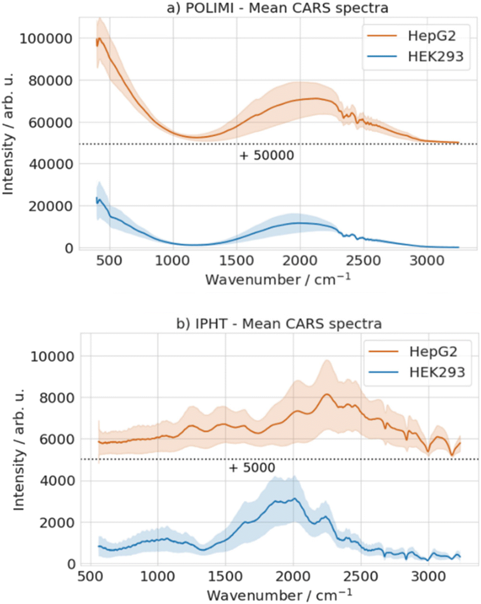Fig. 3 Mean CARS spectra retrieved from the BCARS images acquired at (a) POLIMI and (b) IPHT. An offset of 50 000 was added for HepG2 spectra for POLIMI data and 5000 for IPHT data. The standard deviations in the data were estimated to be over 112 replicates for HepG2, 136 for HEK293 cells for POLIMI data, 41 replicates for HepG2, and 42 for Hek293 cells for IPHT data. The spectra of the same cell type look different between the two setups due to the drastic difference in the reference NRB spectrum.

2.6 Raman signal retrieval from BCARS spectra

It is visually demonstrated that the NRB has a significant effect on the recorded CARS signals. In order to retrieve the resonant signal (i.e., the spectrum of the imaginary part of the third-order non-linear susceptibility, similar to the spontaneous Raman signal) from the measured CARS spectra, the NRB is removed by applying the time-domain Kramers–Kronig (KK) algorithm.²² For this task, we utilized an open-source algorithm in python²⁷ that is described in Camp et al.²³ Also, the reference for this task is the average reference spectrum obtained from the reference mask, as shown in Fig. 2 (orange polygons). The TDKK algorithm consists of three main steps: (i) The first step retrieves the phase of the CARS/NRB signal by applying a windowed Hilbert transform. (ii) The second step is a phase detrending step that corrects for the phase distortions introduced by considering the NRB spectrum as a reference spectrum on glass that does not correspond to the real non-resonant contribution of the cell. (iii) The last step corrects the amplitude distortions, and the error introduced by the use of the windowed Hilbert transform via unity-centering of the real component of the retrieved (phase-corrected) spectrum.

For better correction, we extracted a reference spectrum for each image by selecting a cell-free area within each FOV. This process has been repeated for all measured cells, mainly those with easily distinguishable edges, as shown in Fig. 2. The average of the retrieved Raman spectra was calculated over the entire two batches for each cell line and each setup; the results are presented in Fig. 4. In the spectra obtained from cells measured by the POLIMI BCARS setup, a broad peak beyond 3000 cm⁻¹ is observed, originating from the OH-stretching of water.

Fig. 4 Mean of the Raman spectra retrieved from the BCARS data acquired at (a) POLIMI and (b) IPHT. An offset value of 1 and 0.2 is added to the HepG2 spectra for the POLIMI and IPHT data, respectively. A spectral band is observed after 3000 cm⁻¹ in the POLIMI data due to the water.

Despite using a reference spectrum from the cell-free region containing PBS medium, the remaining peak in the reconstructed spectra associates with a higher concentration of water from within the cells to their surroundings. Conversely, in the case of the Jena BCARS setup, the signal beyond 3000 cm⁻¹ is notably weak, and the reconstruction through KK does not retrieve this signal. Also, the wavenumber and intensity ranges differ between both setups. Further, it is worth considering that, even though the parameters of the reconstruction are chosen the same, the different ratio between the signal and NRB of different samples can lead to differences in the reconstructed spectra, as studied in our recent work.²⁸ Therefore, to ensure consistency and comparability across datasets from different experimental setups, we standardized the spectral data through preprocessing in the following section.

2.7 Preprocessing of retrieved and spontaneous Raman spectra

The retrieved Raman spectra were preprocessed using RAMANMETRIX software developed by our group.²⁹ First, the same spectral range is considered for both setups. The cosmic rays were identified using a spike detection algorithm and replaced with a median-smoothed spectrum.³⁰ Subsequently, the background was corrected using the statistics-sensitive nonlinear iterative peak-clipping (SNIP) algorithm.³¹ In the last step, L2 normalization was applied, and the final preprocessed Raman spectra are shown in Fig. 5.

Fig. 5 Mean preprocessed Raman spectra: (a) POLIMI data and (b) IPHT data. An offset value of 0.25 is added to the HepG2 spectra for better visualization.

It is observed that the spectral variations (shaded area) for each cell line reduced after preprocessing.

In the case of spontaneous Raman data, preprocessing was performed using RamApp.³² The same preprocessing steps were applied, and the final mean processed spontaneous Raman spectra are shown in Fig. 6. It is found that variations are very low in spontaneous Raman spectra compared to the Raman spectra retrieved from the BCARS spectra. An inset is added for each cell line to visualize these small variations, as shown in Fig. 6. Overall, this preprocessing step demonstrated the minimization of spectral variations in the Raman data.

Fig. 6 Mean preprocessed spontaneous Raman spectra of two cell lines. Standard deviations (SD) in the data were estimated over 30 replicates for each cell line. The SD is very small, so part of the spectrum (1300–1520 cm⁻¹) is presented in insets for better visualization.

3. Results and discussion

3.1 Pearson correlation analysis

First, the mean over the entire preprocessed dataset (the average of preprocessed Raman spectra of both the HepG2 and HEK293 cell lines) of each setup is estimated for comparison. The resultant mean over spectra is presented in Fig. 7a. The two spectra on the top correspond to the Raman spectra retrieved from the BCARS data acquired at POLIMI and IPHT, respectively. The third spectrum at the bottom is the spontaneous Raman data.

Fig. 7 (a) Mean spectra estimated over the entire dataset (comprising spectra from both HepG2 and HEK293 cells) of preprocessed Raman data. The shaded area represents the standard deviation calculated from the entire dataset for each setup. The first two rows depict Raman spectra retrieved from BCARS data acquired at POLIMI and IPHT, respectively, while the last spectrum represents spontaneous Raman data. Offset values of 0.25 and 0.5 were added for improved visualization. (b) The Pearson correlation coefficients (PCC) estimated among these three datasets. ‘S_Raman’ represents the spontaneous Raman data. The correlation matrix is symmetric; hence, only the lower diagonal is presented.

All the major vibrational spectral bands in the retrieved Raman spectra matched the spectral bands of the spontaneous Raman data. It confirms that the KK algorithms correctly retrieved all the spectral bands. However, minor variations in peak intensities are observed. For example, the intensity of the spectral band at 1451 cm⁻¹ is higher than the peak at 1661 cm⁻¹ for the spontaneous Raman data. Conversely, an inverse trend is observed for the Raman spectra retrieved from IPHT BACRS data. Meanwhile, both peaks demonstrate nearly identical intensities in the Raman spectra retrieved from the POLIMI BCARS data. Overall, it is noticed that the spectral variations from the spontaneous Raman measurement are lower, with a higher signal-to-noise ratio compared to the remaining two data sets.

Further, the Pearson correlation coefficient (PCC) is calculated to numerically quantify the similarity between the spectra,^33,34 and the results are depicted in Fig. 7b. The retrieved PCC value of more than 0.96 indicates a substantial resemblance of the retrieved spectra to the spontaneous Raman spectra. It also ascertains the performance of the KK algorithm. Furthermore, it is evident that the two retrieved datasets exhibit a higher correlation of 0.98 with each other compared to them with the spontaneous Raman spectrum. In the next section, PCA-LDA analysis is performed to quantify the biological variance in the data.

3.2 Principal-component analysis (PCA) – linear-discriminant analysis (LDA)

In this section, Principal-component analysis (PCA) followed by linear-discriminant analysis (LDA) is applied as a classification model to separate the two cell lines of each dataset.^35,36 PCA is an unsupervised technique that reduces high-dimensional input data into a lower-dimensional space with minimal loss of information. Its objective is to find the directions of maximum variance in a dataset, referred to as principal components (PCs). PC1, the first principal component, captures the most variance present in the data. Subsequent PCs (PC2, PC3, and PC4, etc.) are orthogonal to the previous ones and capture the remaining variance in decreasing order. These PCs serve as inputs to LDA, a supervised method that further reduces data dimensionality by maximizing the ratio between inter-group separation and intra-group variance, ultimately enhancing classification accuracy.

Further, batch-out CV and 10-fold CV is considered for the analysis. In a 10-fold CV, the dataset is divided into ten folds, and the LDA model is trained on nine of these folds and tested on the remaining fold. This process is repeated ten times, with each fold serving as the test set exactly once, and finally, the average accuracy is estimated. In the case of the Batch-out CV, given the two batches of data available for each cell line, one batch is utilized for training and another for testing. Each batch is used once as testing data, and the average accuracy of the cross-validation is estimated. Initially, PCA is applied to each preprocessed dataset, and the corresponding PCs are obtained.

Fig. 8a visualizes the loadings of the first 3 PCs obtained on the preprocessed Raman data retrieved from the POLIMI CARS data. Then, these PCs, serving as features, are systematically chosen as input to construct a linear LDA classifier with a maximum limit of 50 PCs. The model's accuracy is then assessed iteratively for different numbers of PCs, as depicted in Fig. 8b. The optimal number of PCs required for the final classification model was determined using balanced accuracy as the primary metric. It is calculated as the arithmetic mean of the per-class accuracies, where the accuracy of each class is defined as the ratio of correctly predicted instances to the total number of instances in that class.

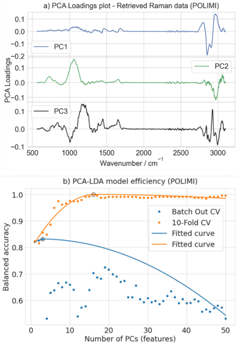Fig. 8 (a) PCA loadings obtained from the preprocessed Raman spectra retrieved from POLOMI BACRS data. PC1, PC2, and PC3 correspond to the first three principal components (PC). (b) Balanced accuracy estimated with the number of PCs as input to construct the LDA classifier. The dots represent the balanced accuracy, and the solid line represents a curve fitted using the 3-piece linear function. The black circle on the fitted curve represents the optimal number of PCs used to create the final LDA classifier, and the corresponding accuracy is utilized for the comparison.

Fig. 8b illustrates the balanced accuracy estimated as a function of the number of PCs input to the LDA classifier. The dots on the graph represent balanced accuracy values, while the solid line represents a curve fitted to those values using a 3-piece linear function.²⁹ This function utilizes a piecewise linear model with three segments to capture different trends in the data and identifies a breakpoint, as shown in Fig. 8b with a black circle. The number of PCs at this point can be considered optimal, and the corresponding accuracy is utilized for further analysis. For instance, 16 PCs are optimal for a 10-fold CV where the estimated balanced accuracy is 100%, which decreases with a further increase in PCs. In the case of batch-out CV, three PCs are found to be optimal, and the corresponding accuracy is 83.3%. This approach not only effectively balances the model complexity and performance but also mitigates the risk of overfitting, ensuring the efficiency of the LDA-based classification model.

The same procedure is applied to the remaining two datasets (1. Raman data retrieved from the IPHT CARS data and 2. Spontaneous Raman data). The corresponding loadings and balanced accuracy curves are presented in ESI Fig. 3 and 4,† respectively. The Raman data retrieved from the IPHT CARS spectra has given the accuracy of 92.7% for batch-out CV and 100% for 10-fold CV. It was also noticed that 7 PCs were found to be optimal for both CV methods. On the other hand, the accuracy of spontaneous Raman data was found to be 100% for both validation methods with optimal PCs of 12.

Further, the loadings represent the coefficients of the original variables in the PCs. Higher loading values indicate a stronger influence of the corresponding variable on the PC.

For example, both fingerprint and CH band regions exhibit higher loading values in all three PCs, as illustrated in Fig. 8a. The same scenario is observed for the remaining two datasets (1. Raman data retrieved from the IPHT CARS data and 2. Spontaneous Raman data), as shown in ESI Fig. 3a and 4a.† These loading plot visualizations underscore the significance of the fingerprint region and, particularly, the CH band region in classifying cell lines for all three datasets. This observation suggests that a PCA-LDA model based on selected spectral regions could be more effective, helping to mitigate the influence of noisy regions within the spectrum. Hence, the PCA-LDA analysis is done by considering different regions of the spectrum as an input to the model, as illustrated in Fig. 9.

Fig. 9 Different regions of the Raman spectrum considered as the input to the PCA-LDA analysis. First, the entire spectrum is divided into fingerprint (600–1800 cm⁻¹) and CH band (2770–3070 cm⁻¹) regions. Then, the fingerprint region is equally subdivided into four parts or sub-spectra (S1, S2, S3, and S4). Overall, 11 specified regions (S1, S2, S3, S4, CH, F, F-CH, S1-CH, S2-CH, S3-CH, and S4-CH) were selected as input for PCA-LDA model.

Initially, the entire spectrum was divided into fingerprint (F) and CH band (CH) regions guided by the outcomes of the loading plot visualizations. The exclusion of the silent region (1800–2770 cm⁻¹) from the analysis was imperative as it predominantly contains noise. Then, the fingerprint region (600–1800 cm⁻¹) was subdivided into sub-spectra (S1, S2, S3, and S4), each highlighting specific peaks and having a bandwidth of 300 cm⁻¹.

For example, the S1 region mainly contains the characteristic peak of nucleic acids at 785 cm⁻¹ associated with the symmetric phosphodiester stretch.³⁷ The S2 region displays three major peaks at 934, 1004, and 1094 cm⁻¹, which are characteristic of nucleic acids and lipids.³ The last two frequencies specifically denote the ring breathing modes and phosphate backbone vibrations, respectively. The S3 region contains vibrational features of both proteins and lipids. The peak at 1240 cm⁻¹ belongs to the Amide-III band, associated with protein content. Additionally, the peaks at 1338 and 1450 cm⁻¹ represent the CH₂ bending modes, indicating lipid content. Finally, the last region, S4, contains an Amide-I band at 1654 cm⁻¹ with higher intensity, primarily associated with C=O stretching vibrations of peptide bonds in proteins.³⁸ Further, the CH band, in conjunction with the other regions, was also considered, resulting in F-CH, S1-CH, S2-CH, S3-CH, and S4-CH combinations In total, 11 specified regions (S1, S2, S3, S4, CH, F, F-CH, S1-CH, S2-CH, S3-CH, and S4-CH) were used as input for PCA-LDA each time, and the balanced accuracies were estimated. Finally, the results were compared with the accuracy obtained using the total data as input.

Fig. 10 illustrates the batch-out CV analysis results where the spontaneous Raman data has demonstrated superior performance compared to IPHT and POLIMI data for any spectral combination. Notably, a 100% classification accuracy was achieved for all inputs of spontaneous Raman data, excluding specific sub-spectrum regions. Even within these sub-spectrum regions, the minimum accuracy was found to be more than 96.5%. In contrast, a different scenario was observed for the two BCARS datasets, where the accuracy significantly varied based on the input data. Additionally, it was observed that the IPHT BCARS data consistently showed higher accuracy than the POLIMI data for all combinations, except in the S3 and S4 regions.

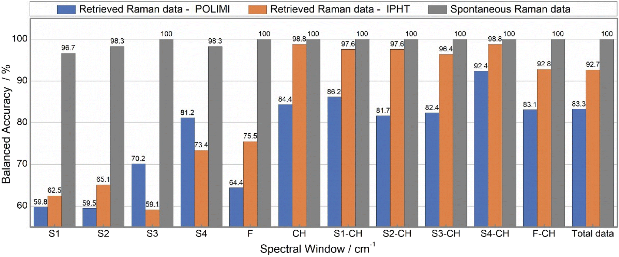Fig. 10 Comparison of balanced accuracies obtained from PCA-LDA analysis using batch-out CV. For each cell line, two batches of the data were used for the analysis. The highest classification accuracy is achieved for spontaneous Raman data across all the inputs. In the remaining two datasets, the IPHT has given more accuracy than POLIMI data for all the inputs except for the S3 and S4 regions. Also, it is noticed that any combination involving the CH band improved accuracy, and the S4-CH combination has given the highest classification accuracy among all the inputs and across all three datasets.

Further, the fingerprint region exhibited lower accuracy compared to the CH band. Also, any combination involving the CH band as an input demonstrated increased accuracy. For example, POLIMI data accuracy in the S1 region improved from 59.8% to 86.2% when combined with the CH band. Similarly, for IPHT data, accuracy increased from 62.5% to 97.6%, and spontaneous Raman data increased from 96.7% to 100%. This trend was consistently observed for all remaining combinations. Particularly, the S4-CH combination exhibited the highest accuracy, surpassing that achieved with the total data as an input to the model. For instance, POLIMI total data accuracy was only 83.3% and increased to 92.4% for the S4-CH combination. It is worth considering that the same scenario was noticed for the remaining two datasets (1. Raman data retrieved from the IPHT CARS data and 2. Spontaneous Raman data).

The same analysis is repeated for the 10-fold CV, and the results are presented in Fig. 11. An overall increase in accuracy is observed compared to the results obtained through batch-out CV. However, the key distinction lies in the intricacies of the 10-fold CV procedure. Due to the random partitioning of the entire dataset (two batches of data), there exists a higher likelihood of data overlap or leakage from one batch to another within the individual folds. This contrasts with the batch-out CV method, explicitly designed to mitigate biases by segregating distinct batches for training and testing, providing an unbiased and stringent estimate of the model's performance. Hence, the lower accuracy in batch-out CV is attributed to batch variance present in each cell for all three data sets. Also, similar observations were noticed in our previous works.³⁹

Fig. 11 Comparison of balanced accuracies obtained from the PCA-LDA analysis using 10-fold CV. 100% accuracy is achieved for all datasets when the total data and S4-CH region are given as input. Spontaneous Raman data demonstrate 100% accuracy for all inputs, excluding the S4 region. Additionally, any combination involving the CH band exhibits improved accuracy, with the S4-CH combination showing the highest accuracy across all three datasets. Moreover, the regions CH, S1-CH, S2-CH, S3-CH, and F-CH also yield 100% accuracy for spontaneous Raman data and IPHT data, albeit slightly lower for POLIMI.

In the case of spontaneous Raman data, 100% classification accuracy was obtained for all inputs except the S4 region. Even the S4 region has demonstrated an accuracy of 98.3%. Additionally, both the total data and the S4-CH combination have demonstrated 100% accuracy across all three datasets. Further, the remaining combinations involving CH also achieved 100% accuracy for Spontaneous Raman and IPHT data, with only a negligible difference observed for the POLIMI data, where the accuracy differed by approximately 1%. Overall, accuracies varied between 78–90% for the sub-spectrum regions of the POLIMI and IPHT data, with the minimum observed for the S1 region and the maximum for the S4 region. The insights derived from both CV methods demonstrate that adopting a targeted region approach, e.g., focusing solely on the CH band or the combined S4-CH region, can minimize the data acquisition times and is particularly helpful for improving the efficiency of imaging applications.

Even though the present study has supported the understanding and quantification of biological variance in BCARS data of HepG2 and HEK293 cell lines, there are avenues for further research to enhance the applicability of BCARS in biomedical investigations. First, exploring additional cell lines with more batches of the data and experimental conditions could provide a more comprehensive understanding of the generalizability of our findings. Investigating the influence of specific cellular components on spectral variations would deepen insights into the molecular basis of biological variance.

Further, it is worth considering that the variance can be introduced from the biological sample, preprocessing (including phase retrieval), and the CARS measurement devices. The present study is primarily focused on the biological aspect (which is probably higher than the other two, at least for spontaneous Raman spectra). The second aspect is also addressed by applying the proper preprocessing steps. Finally, the last part requires a ring trial like we did for Raman spectra to check the influence of the CARS device and its data processing on the spectral data, leading to an understanding of the compatibility.^40,41 Also, in the future, deep learning (DL) models can be explored for efficient removal of NRB and retrieval of resonant Raman information.^17,42,43 Pursuing these future directions holds the potential to refine our understanding of BCARS spectroscopy and its application in biomedical research, ultimately advancing our ability to harness spectroscopic imaging for meaningful insights into biological systems.

4. Conclusions

This systematic study on two cell lines (HEK 293 and HepG2) has provided valuable insights into estimating the biological variance in BCARS data. The data preprocessing approach reduced the variations in the spontaneous Raman data and Raman data retrieved from BCARS spectra. The Pearson correlation analysis demonstrated that the retrieved Raman spectrum is in good agreement with the spontaneous Raman spectrum. In PCA-LDA analysis, 100% accuracy was achieved for three datasets in the 10-fold CV. However, it decreased in batch out CV, which is 83.3% for POLIMI data and 92.7% for the IPHT data. A large difference between 10-fold and batch-out CV accuracy suggests significant batch variations present in the data. Further, the PCA-LDA analysis with different spectral regions as input revealed that the CH band region (2770–3070 cm⁻¹) consistently emerged as a crucial contributor to accurate classification. Notably, the combination of the CH band and the sub-spectrum S4 region (1500–1800 cm⁻¹) exhibited 100% balanced accuracies across all three datasets in a 10-fold CV. In batch-out CV, 92.4% accuracy was obtained for the POLIMI dataset and 98.8% for the IPHT dataset. These observations suggest that the S4-CH combination could be a more robust region to reduce the influence of batch variations of HepG2 and HEK293 cell lines. In summary, our work not only enhances the understanding of biological variance in BCARS but also offers a valuable framework for optimizing spectral analysis in biomedical research. Moreover, this study contributes to the advancement of BCARS as a spectroscopic imaging tool, providing a foundation for future research in characterizing cellular structures and lipid distributions.

Author contributions

Rajendhar Junjuri: formal analysis, visualization, methodology, writing – original draft, and writing – review & editing. Matteo Calvarese, MohammadSadegh Vafaeinezhad, Federico Vernuccio, and Marco Ventura: investigation, writing – review & editing. Benedetta Gavazzoni, Silvia Ghislanzoni and Matteo Negro: data curation. Italia Bongarzone: data curation, writing – review & editing. Tobias Meyer-Zedler, Dario Polli, Renzo Vanna, Juergen Popp, and Thomas Bocklitz: methodology, conceptualization, funding acquisition, resources, writing – review & editing.

Data availability

Data for this article, including metadata are available at Zenodo at https://doi.org/10.5281/zenodo.12698413.

Conflicts of interest

There are no conflicts to declare.

Acknowledgements

This work is supported by the EU funding program with grant numbers 101016923 (CRIMSON), 101058004 (CHARM) and 860185 (PHAST). This work is supported by the BMBF, funding program Photonics Research Germany (LPI (FKZ:13N15466, 13N15706, 13N15464)) and is integrated into the Leibniz Center for Photonics in Infection Research (LPI). The LPI initiated by Leibniz-IPHT, Leibniz-HKI, UKJ, and FSU Jena is part of the BMBF national roadmap for research infrastructures.

References

1. S. H. Parekh, Y. J. Lee, K. A. Aamer and M. T. Cicerone, Biophys. J., 2010, 99, 2695–2704.
2. A. Volkmer, J. Phys. D: Appl. Phys., 2005, 38, R59–R81.
3. T. Tolstik, C. Marquardt, C. Matthaus, N. Bergner, C. Bielecki, C. Krafft, A. Stallmach and J. Popp, Analyst, 2014, 139, 6036–6043.
4. R. Vanna, A. De la Cadena, B. Talone, C. Manzoni, M. Marangoni, D. Polli and G. Cerullo, Riv. Nuovo Cimento, 2022, 45, 107–187.
5. C. Krafft, B. Dietzek, M. Schmitt and J. Popp, J. Biomed. Opt., 2012, 17, 040801.
6. L. G. Rodriguez, S. J. Lockett and G. R. Holtom, Cytometry, Part A, 2006, 69, 779–791.
7. R. Junjuri, A. Saghi, L. Lensu and E. M. Vartiainen, RSC Adv., 2022, 12, 28755–28766.
8. A. Saghi, R. Junjuri, L. Lensu and E. M. Vartiainen, Opt. Continuum, 2022, 1, 2360–2373.
9. T. Guerenne-Del Ben, Z. Rajaofara, V. Couderc, V. Sol, H. Kano, P. Leproux and J. M. Petit, Sci. Rep., 2019, 9, 13862.
10. S. W. Li, Y. P. Li, R. X. Yi, L. W. Liu and J. L. Qu, Front. Phys., 2020, 8, 598420.
11. D. Polli, V. Kumar, C. M. Valensise, M. Marangoni and G. Cerullo, Laser Photonics Rev., 2018, 12, 1800020.
12. C. Krafft, B. Dietzek and J. Popp, Analyst, 2009, 134, 1046–1057.
13. C. H. Camp Jr., Y. J. Lee, J. M. Heddleston, C. M. Hartshorn, A. R. Hight Walker, J. N. Rich, J. D. Lathia and M. T. Cicerone, Nat. Photonics, 2014, 8, 627–634.
14. G. I. Petrov, R. Arora and V. V. Yakovlev, Analyst, 2021, 146, 1253–1259.
15. F. Vernuccio, A. Bresci, B. Talone, A. de la Cadena, C. Ceconello, S. Mantero, C. Sobacchi, R. Vanna, G. Cerullo and D. Polli, Opt. Express, 2022, 30, 30135–30148.
16. H. A. Rinia, K. N. Burger, M. Bonn and M. Muller, Biophys. J., 2008, 95, 4908–4914.
17. R. Junjuri, A. Saghi, L. Lensu and E. M. Vartiainen, Phys. Chem. Chem. Phys., 2023, 25, 16340–16353.
18. N. Coluccelli, G. Galzerano, P. Laporta, K. Curtis, C. L. Lonsdale, D. Padgen, C. R. Howle and G. Cerullo, Sci. Rep., 2023, 13, 2634.
19. A. Khmaladze, J. Jasensky, E. Price, C. Zhang, A. Boughton, X. Han, E. Seeley, X. Liu, M. M. Banaszak Holl and Z. Chen, Appl. Spectrosc., 2014, 68, 1116–1122.
20. V. A. Arzumanian, O. I. Kiseleva and E. V. Poverennaya, Int. J. Mol. Sci., 2021, 22, 13135.
21. J. Hu, J. Han, H. Li, X. Zhang, L. L. Liu, F. Chen and B. Zeng, Cells Tissues Organs, 2018, 205, 1–8.
22. V. Lucarini, J. J. Saarinen, K.-E. Peiponen and E. M. Vartiainen, Kramers-Kronig relations in optical materials research, Springer Science & Business Media, 2005.
23. C. H. Camp Jr, Y. J. Lee and M. T. Cicerone, J. Raman Spectrosc., 2016, 47, 408–415.
24. F. Vernuccio, R. Vanna, C. Ceconello, A. Bresci, F. Manetti, S. Sorrentino, S. Ghislanzoni, F. Lambertucci, O. Motino, I. Martins, G. Kroemer, I. Bongarzone, G. Cerullo and D. Polli, J. Phys. Chem. B, 2023, 127, 4733–4745.
25. A. Bresci, J. H. Kim, S. Ghislanzoni, F. Manetti, L. Wu, F. Vernuccio, C. Ceconello, S. Sorrentino, I. Barman, I. Bongarzone, G. Cerullo, R. Vanna and D. Polli, Sci. Adv., 2023, 9, 1–16.
26. F. Masia, A. Glen, P. Stephens, P. Borri and W. Langbein, Anal. Chem., 2013, 85, 10820–10828.
27. C. H. Camp. Jr, CRIKit2: Hyperspectral imaging toolkit, 2024, https://github.com/CCampJr/CRIkit2.
28. R. Junjuri, T. Meyer, J. Popp and T. Bocklitz, 2024, preprint, arXiv:2406.17829,  DOI:10.48550/arXiv.2406.17829.
29. D. Storozhuk, O. Ryabchykov, J. Popp and T. Bocklitz, 2022, preprint, arXiv:2201.07586,  DOI:10.48550/arXiv.2201.07586.
30. T. Kirchberger-Tolstik, O. Ryabchykov, T. Bocklitz, O. Dirsch, U. Settmacher, J. Popp and A. Stallmach, Analyst, 2021, 146, 1239–1252.
31. C. G. Ryan, E. Clayton, W. L. Griffin, S. H. Sie and D. R. Cousens, Nucl. Instrum. Methods Phys. Res., Sect. B, 1988, 34, 396–402.
32. Ramapp, https://ramapp.io/, 2024.
33. A. Z. Samuel, R. Mukojima, S. Horii, M. Ando, S. Egashira, T. Nakashima, M. Iwatsuki and H. Takeyama, ACS Omega, 2021, 6, 2060–2065.
34. R. Junjuri, A. Saghi, L. Lensu and E. M. Vartiainen, Opt. Continuum, 2022, 1, 1324–1339.
35. N. Ali, S. Girnus, P. Rosch, J. Popp and T. Bocklitz, Anal. Chem., 2018, 90, 12485–12492.
36. C. W. Park, I. Lee, S. H. Kwon, S. J. Son and D. K. Ko, Vib. Spectrosc., 2021, 117, 103314.
37. X. Zhang, M. B. Roeffaers, S. Basu, J. R. Daniele, D. Fu, C. W. Freudiger, G. R. Holtom and X. S. Xie, ChemPhysChem, 2012, 13, 1054–1059.
38. K. Moor, Y. Terada, A. Taketani, H. Matsuyoshi, K. Ohtani and H. Sato, J. Biomed. Opt., 2018, 23, 1–7.
39. S. X. Guo, T. Bocklitz, U. Neugebauer and J. Popp, Anal. Methods, 2017, 9, 4410–4417.
40. S. Guo, C. Beleites, U. Neugebauer, S. Abalde-Cela, N. K. Afseth, F. Alsamad, S. Anand, C. Araujo-Andrade, S. Askrabic and E. Avci, Anal. Chem., 2020, 92, 15745–15756.
41. F. Hempel, F. Vernuccio, L. König, R. Buschbeck, M. Rüsing, G. Cerullo, D. Polli and L. M. Eng, Appl. Opt., 2024, 63, 112–121.
42. R. Houhou, P. Barman, M. Schmitt, T. Meyer, J. Popp and T. Bocklitz, Opt. Express, 2020, 28, 21002–21024.
43. C. M. Valensise, A. Giuseppi, F. Vernuccio, A. De la Cadena, G. Cerullo and D. Polli, APL Photonics, 2020, 5, 061305-1–061305-8.

---

Footnote

† Electronic supplementary information (ESI) available: For the Supplementary Fig. 1–4. See DOI: https://doi.org/10.1039/d4an00648h

---