
 Open Access Article
 This Open Access Article is licensed under a Creative Commons Attribution-Non Commercial 3.0 Unported Licence
Relationship between air pollutant distribution and large-scale circulation
Yassin
Mbululo
 *ab,
Qin
Jun
b,
Fatuma
Nyihirani
c,
Zhengxuan
Yuan
b,
Sijing
Huang
b and
Yajuan
Wang
b
*ab,
Qin
Jun
b,
Fatuma
Nyihirani
c,
Zhengxuan
Yuan
b,
Sijing
Huang
b and
Yajuan
Wang
b
aDepartment of Geography and Environmental Studies, College of Natural and Applied Sciences, PO Box 3038, Morogoro, Tanzania. E-mail: ymbululo@sua.ac.tz
bDepartment of Atmospheric Science, School of Environmental Studies, China University of Geosciences (Wuhan), Hubei 430074, China
cInstitute of Development Studies, Center for Environment, Poverty and Sustainable Development, Mzumbe University, Morogoro, Tanzania
First published on 26th June 2023
Abstract
The Antarctic Oscillation (AAO) has long been linked to the weather and climate of the Northern Hemisphere (NH); however, its linkage with pollutant distribution in China has seldom been discussed. In this study, using the boundary layer structure index (BLSI), NOAA–ESRL and NCEP/NCAR reanalysis data, the effect of boreal summer AAO on pollutant distribution was studied. Regarding the relationship between AAO and pollutant distribution, the Antarctic Oscillation Index (AAOI) was correlated with the dust surface mass concentration (DSMC) of PM2.5 over China, in which boreal summer (June and July) AAO signals (JJ–AAOI) were selected as the determinant leading factor in establishing a relationship with pollutants during boreal winter (from November to February). The results show that the average of JJ–AAOI has a significant correlation with the DSMC of PM2.5. August–October were the most significant months over the Antarctic, as indicated by their large coverage of significant areas compared to the coverage of other months. These findings imply that the signals of JJ–AAOI can be stored in Antarctic sea ice up to August–October before they affect the atmospheric boundary layer (ABL), which ultimately affects pollutant distribution in the end. The analysis of the relationship between the DSMC of PM2.5 and large-scale circulation first involved the use of the empirical orthogonal function (EOF) of the decomposed winter DSMC of PM2.5. The time series from the EOF1 analysis showed a wave train of four years of positive and negative (+, −, +), followed by a decadal negative value. Moreover, the analysis of the composite difference of meridional circulation between the years of high and low JJ–AAOI shows significant ascending and southerly anomalies at around 25 °N and 35 °N during the higher JJ–AAOI years. These results act as a good starting point for the effort to develop a comprehensive forecasting model for pollutant distribution.
Environmental significanceThis study is environmentally significant because it revealed the dynamics of the atmospheric boundary layer structure (ABLS), the Antarctic Oscillation Index (AAOI) and its relationship with air pollution. It is noteworthy that air pollution is a serious problem in most developing countries, and special efforts are needed to overcome it. In this study, we found a linkage between pollutant distribution in mainland China and large-scale circulation. An identified area with a high correlation over Antarctic sea ice is a good starting point in the effort to develop a comprehensive forecasting model for pollutant distribution in mainland China. |
Introduction
Air pollution is a major global public health concern. This has been reflected in a published report by the World Health Organization (WHO) indicating that only 10% of people live in cities, conforming to the WHO air quality guidelines. What is shocking is that air pollution causes the death of one in every nine people annually and outdoor air pollution is responsible for the death of 3 million people every year.1 An updated report from the WHO suggests that the situation is becoming worse because in 2016, ambient air pollution caused about 4.2 million deaths, while household cooking polluting fuels caused about 3.8 million death.2 The report further shows that more than 1.2 billion people worldwide are still using polluting household cooking fuel and technologies, which are the main sources of indoor and outdoor pollution.Thus far, China is the fastest-growing country in the world at a pace that has never been seen before. This growth is partially due to heavy investments in the manufacturing industries of different kinds of products. This has an impact on air pollution because most of these industries use coal as one of the major sources of power; the habitual use of coal for heating households by rural dwellers also contributes to the impact.3,4 Moreover, lifestyle changes caused by changes in economic status, such as an increase in the number of vehicles, as seen in most Chinese cities, worsen the air quality status of the country to a greater extent. In addition, unfavourable meteorological conditions have been documented as other factors. For instance, Han et al.5 in Tianjin reported the difference in concentrations of PM2.5, PM10, NOx, and SO2 to be about 2- and 4-fold higher during haze days than during non-haze days. A study by Yang et al.6 on PM2.5 concentration and speciation in megacities in China shows pronounced variations in the concentration of about six-fold, where higher concentrations were dominant in northern and western parts while the lower concentrations were common in remote areas and Hong Kong. However, several studies have reported that the air quality of Wuhan7–10 and China11–14 is worse, as it does not meet air quality standards.
This has reinforced the Chinese government to make efforts to mitigate the air pollution problem, including the enactment of a stringent law (National Ambient Air Quality Standard (NAAQS)) in 2012 to curb the emission of air pollutants. The NAAQS stipulates the hourly, daily and annual standards of NO2, SO2, CO, O3, PM10 and PM2.5; the PM10 and PM2.5 represent particulate matter with aerodynamic diameters of less than 10 microns and 2.5 microns, respectively. Thus far, several studies on boundary layer structure, which is the main determinant of air pollutants, are available online.15–20 Apart from the pioneer studies21–24 on pollutant forecasting using large-scale circulations, little has been done in this area, which is the key to planning and pollutant management. This study, therefore, aims at highlighting the relationship between pollutant distribution and large-scale circulation, which is potential for forecasting pollutants.
Methodology
Boundary layer data
This study used the boundary layer structure index (BLSI), which was developed by Zheng et al.20 This index can effectively describe the atmospheric boundary layer (ABL) and ground air quality. The index uses daily L-band sounding data for temperature, relative humidity, and wind speed and direction with a vertical resolution range of 10 m–3000 m to describe the vertical profile of the ABL. The L-band data are collected three times daily at 0200 LST, 0700 LST, and 1900 LST, but the first data lack wind direction. Thus, the 0200 LST data were the first to be excluded. It is noteworthy that before sunrise, the loss of longwave radiation is at the maximum level and the atmospheric stratification is mostly stable. Therefore, the atmospheric diffusion conditions at 0700 LST are always worse than those at 1900 LST owing to the stability conditions of the atmosphere. Consequently, this study opted to use the L-band data at 0700 LST as a representative of the condition of the ABL. Note that BLSI can define the conditions of the lower atmosphere and changes in ground air quality. This index (BLSI) considers that both the horizontal removal and vertical diffusion ability of ABLS can effectively represent the condition of the lower atmosphere. Therefore, it is appropriate to use it to characterize pollutant distribution in a lower atmosphere. The data for air quality were made available by the Wuhan Environmental Protection Agency (WHEPA), and the L-band sounding data were acquired from the Cihui farm station (CFS), which was administered by the Wuhan Meteorological Bureau (WMB). The equation of BLSI, following Zheng et al.,20 is as follows: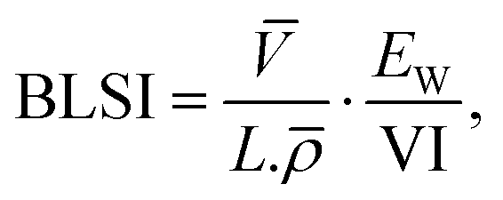 | (1) |
![[V with combining macron]](https://www.rsc.org/images/entities/i_char_0056_0304.gif) represents the average wind speed at ground level (0 m) and at height (H m) (m s−1), L represents the condensation latent heat value of water vapour (2500.6 J g−1),
represents the average wind speed at ground level (0 m) and at height (H m) (m s−1), L represents the condensation latent heat value of water vapour (2500.6 J g−1), ![[small rho, Greek, macron]](https://www.rsc.org/images/entities/i_char_e0d1.gif) denotes the average air density at ground level and H m (kg m−3), EW denotes the stable energy from the ground to height H (J cm−2) and VI represents the ventilation index (m2 s−1).
denotes the average air density at ground level and H m (kg m−3), EW denotes the stable energy from the ground to height H (J cm−2) and VI represents the ventilation index (m2 s−1).
Monthly average data reanalysis
The NCEP/NCAR (National Center for Atmospheric Research) monthly reanalysis means of atmospheric variables, such as geopotential height (GPH), sea level pressure (SLP), vertical velocity (omega), horizontal (u) and meridional (v) wind speed, are provided with a 2.5° × 2.5° grid resolution (https://www.esrl.noaa.gov/psd/data/gridded/index.html).25 The monthly average data of dust surface mass concentration of PM2.5 (kg m−3) were from the National Aeronautics and Space Administration (NASA), Modern-Era Retrospective Analysis for Research and Application, and Version 2 (MERRA-2) (https://gmao.gsfc.nasa.gov/reanalysis/MERRA-2/) with approximately 0.5° × 0.625° resolution. The MERRA-2 dust surface mass concentration of PM2.5 is calculated based on the concentration of five species (i.e., dust, sea salt (SS), black carbon (BC), organic carbon (OC) and sulfate ion (SO4)) with a diameter of less than 2.5 μm14,26–28 given in the following equation:| PM2.5 = 1.375 × [SO4] + 1.6 × [OC] + [BC] + [SS] + [dust]. | (2) |
All data sets were from 1980 to 2018, and the MERRA-2 data are available only from 1980 to the present.29 An empirical orthogonal function (EOF), which is also known as eigenvector analysis, was performed on the MERRA-2 data. Several studies14,27 suggest that these data are reliable for studying air pollution. It is noteworthy that this method can analyze physical features in matrix data, yielding key features. The analysis results can decompose both variable fields, that is, those that depend on the variation of time and those that do not depend only on time variation, into the spatial function. In this study, the anomalies of EOF were normalized before the time series were used in computing the correlations. The AAOI data from 1979 to 2018 were obtained from the NOAA (https://www.esrl.noaa.gov/psd/data/climateindices/list/).30 The AAOI data after the year 1979 are regarded as more accurate data since they are obtained after the satellite era31–34 unlike the data from the pre-satellite era (before the year 1979), which many queries.35 The AAOI data applied here from NOAA use the first leading mode of Empirical Orthogonal Function (EOF1) analysis of monthly mean geopotential height (GPH) anomalies at 700 hPa south of 20° of the equator. Numerous studies32,36,37 suggest that ENSO plays a significant role in climate anomalies, which have been experienced in the North Hemisphere (NH). Therefore, before AAOI was used, a linear detrend method was performed to remove the influence of ENSO (the ENSO index equals the Nino3.4 index). Then, the AAOI was normalized (eqn (3)) to remove the interannual variability of the data. The monthly mean sea ice concentration data from 1982 to 2017 from NOAA (https://www.esrl.noaa.gov/psd/data/gridded/data.20thC_ReanV2c.html) and AAOI data were used to develop the ice index.
 | (3) |
![[X with combining macron]](https://www.rsc.org/images/entities/i_char_0058_0304.gif) is the average value for the entire range of data and S is the standard deviation.
is the average value for the entire range of data and S is the standard deviation.
The singular value decomposition (SVD) analysis was also used to examine the potential covariability between the leading AAOI and the lagging BLSI; the GPH was used from 1000 hPa to 10 hPa south of the equator. The SVD analysis, which is essentially a matrix operation method,38 can describe the spatial correlation patterns of two fields (“left data” and “right data”) temporal covariance. This method can separate the high-correlation modes between two field sequences to the maximum extent. Many studies24,39–41 have used this method in climate diagnosis because it has been observed to be superior to other decomposition methods (i.e., principal component analysis (PCA) and canonical correlation analysis (CCA)).38 In this study, the GPH lagged the BLSI for about three months. Apart from EOF and SVD, other statistical methods used in analyzing the existing relationship between AAOI and pollutant distribution in winter include simultaneous and lead–lag correlation, linear regression, and composite. The identification and selection of the year with high and low indexes (AAOI) were based on the deviation of the index beyond 0.5 times the calculated standard deviation, that is, 0.5 was multiplied by the calculated standard deviation and compared to the obtained mean of the index. In this study, the difference in the corresponding elements between the high- and low-index cases is denoted as a composite difference.
Results and discussion
The boundary layer structure index (BLSI) and the Antarctic Oscillation Index (AAOI)
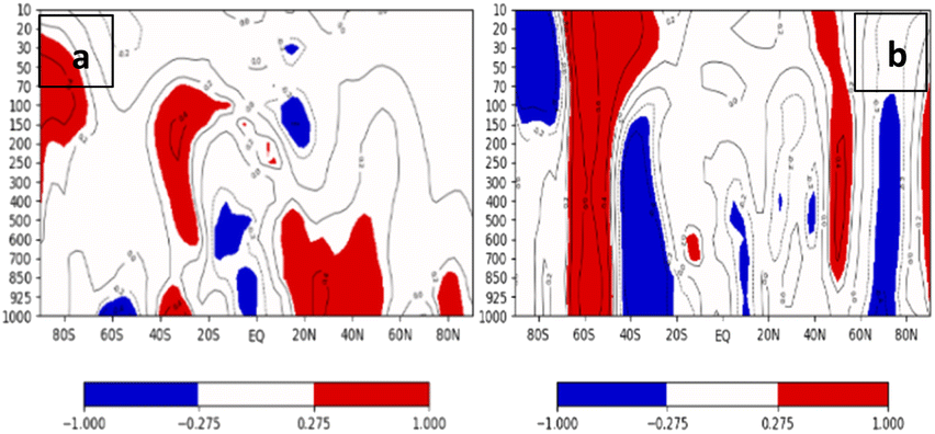
To establish the relationship between pollutants and AAOI, SVD analysis was used to determine the covariance of GPH and BLSI. The lagging GPH from 1000 hPa to 10 hPa was used to depict the AAOI-like features, and the leading BLSI of Wuhan City, China, was calculated based on the method proposed by Zheng et al.20 Similar to BLSI, the GPH characterizes coherent dynamic and thermodynamic components of the atmosphere from the ground level to the troposphere.42 The correlation analysis of GPH for the lagging month of June, July and August (JJA–GPH) and the leading BLSI of December, January and February (DJF–BLSI) was performed. Fig. 1a shows the average BLSI (DJF–BLSI), and Fig. 1b shows the correlation map of the vertical structure of the JJA–GPH. The analysis results show that the coupled pattern of the lagging GPH–SVD and the leading BLSI–SVD can explain 51% of the total squared covariance of DJF–BLSI from the JJA–GPH-like AAO pattern. The higher squared covariance, which is explained by this leading SVD, suggests that this pattern is the primary phenomenon and can significantly influence the leading BLSI in Wuhan. This observation suggests that other modes are secondary phenomena. The positively correlated area, which is significant at the 95% confidence level for the GPH, is situated south of 55 °S throughout the troposphere and at an altitude of 700 hPa to 70 hPa at around 15 °S to the equator (Fig. 1b). Note that the correlated area (55 °S ∼ 90 °S) falls within the area used to define AAOI.43,44 Therefore, this result suggests that the AAOI-like pattern generated by GPH significantly influences pollutant distribution in Wuhan. Previous studies reported a similar lead–lag time scale of AAOI to influence dust mass frequency45 and surface temperature24 over North China. Moreover, the time series of the BLSI and the GPH has a correlation coefficient (r) of 0.49, which is significant at the 95% confidence level (Fig. 1c and d). The positive signals of the leading GPH during June and July coincide with the positive signals of the BLSI during the subsequent months of December and January. Similarly, the negative phase of the leading GPH during August coincides with the negative phase of the BLSI in the subsequent month of February. This lead–lag mechanism is consistent and assents to the proposition that leading JJA–AAOI determines the condition of the BLSI in the subsequent months (December, January and February), which determines the condition of the air quality in the end. | ||
| Fig. 1 The leading mode of the singular value decomposition (SVD) of geopotential height (GPH) and boundary layer structure index (BLSI) showing (a) the average boundary layer structure index from December 2014 to February 2015 (DJF–BLS); (b) the correlation map of the atmosphere showing the hgt south of the equator from June to August 2014 and the BLSI in Wuhan. The shaded area shows the areas that are statistically significant at a 95% confidence level; (c) time series of the BLSI anomaly and (d) time series of the GPH anomaly. | ||
Antarctic Oscillation Index (AAOI) and pollutant distribution
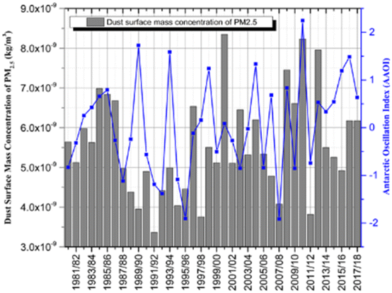
Based on the established covariance of GPH–SVD and BLSI–SVD, it is evident that AAOI significantly influences BLSI, which determines pollutant distribution in the end. Therefore, this subsection correlates the average of June and July AAOI (JJ–AAOI) (i.e., boreal summer) with the average dust surface mass concentration of PM2.5 from November to February (boreal winter). An assessment study on MERRA-2 surface dust mass concentration of PM2.5 conducted by He et al.27 reveals a significant correlation with surface measured PM2.5 over the Yangtze River Basin (YRB). Similar consistent observations between surface measured and MERRA-2 data (dust surface mass concentration of PM2.5) have been reported in North China by Song et al.14 Therefore, MERRA-2 data are reliable data for studying air pollution. It is also noteworthy that November is not a winter month, but during this period, the concentration of PM2.5 is higher, which resembles what is experienced during the winter month (December, January, and February (DJF)). Therefore, November was included in the analysis as the winter month to capture the feedback mechanism of the AAOI. A previous study conducted by Fan and Wang45 on the Antarctic oscillation (AAO) and dust weather frequency found that there was a significant correlation between the AAO of DJF and surface air temperature in North China.The average dust surface mass concentration of PM2.5 over the area (115 °E – 125 °E and 30 °N–40° N), which showed a significant correlation with the AAOI, was determined and used to develop the time series of pollutants with the AAOI. The determined correlation coefficient for this area was 0.42, which is significant at a 95% confidence level. A closer look at the time series of AAOI (Fig. 2) showed a consistent lead–lag effect except in the two scenarios (from 1988/1989 to 1993/1994 and from 2013/2014 to 2017/2018) where the trends were not obvious. The exclusion of these two scenarios shows an increase in the correlation coefficient to 0.57 between AAOI and the average dust mass concentration of PM2.5. The observed trends, which were not obvious, are believed to be so because pollutant distribution over the area is determined by more than one system. Thus, it is possible that other influential systems were stronger during this period than the effects of the AAOI. For instance, a study conducted by Chen and Wang46 suggested that the weakened northerly winds and the growth of inversion anomalies in the lower part of the troposphere and the weakened trough over East Asia are the reason for haze occurrence. Thus, whenever one of the factors of this inter-dependable system changes, the whole system behaves differently from its normal behavior.
 | ||
| Fig. 2 Time series of average dust mass surface concentration of PM2.5 over the area during winter (from November to February of the following year) and the average of June and July Antarctic oscillation index (JJ–AAOI) from 1980 to 2018. | ||
Forecast of dust mass concentration of PM2.5
To further study the ability of the June and July AAOI (JJ–AAOI) to describe changes in the winter dust mass concentration of PM2.5, its potential for forecasting was tested. The linear regression method was used to develop a prediction equation for the dust surface mass concentration of PM2.5 over the region, which showed a positive correlation with the AAOI. The dust surface mass concentration of PM2.5 was detrended and used to develop the anomaly time series of PM2.5 concentration. The data set of thirty years (30) from 1980 to 2009 was used to train the system and to formulate the forecasting equation, while the data from 2010 to 2017 was used to run the prediction equation. Among the different models (linear, quadratic, cubic, exponential, and logarithmic) that were tested, the linear equation model was found to be the best model (figure not shown). The developed linear regression equation was modified by adding a percentage error to the training data set and generating a new regression equation. This procedure was repeated several times to the point where the percentage error was reduced, and a more convincing equation was generated. Note that whenever the process was repeated, new coefficients were generated for the forecast equation. Many studies have also used linear regression equations to forecast weather and climate parameters.47–49 The best linear regression equation is| y = 9.1845x − 1.5146. | (4) |
The dependent variable (y) represents the anomaly of the dust surface mass concentration of PM2.5, while the independent variable (x) represents the average of June and July AAOI (JJ–AAOI).
The predicted trend was almost the same as the measured values of the anomaly of dust surface mass concentration of PM2.5 (Fig. 3) even though the magnitude of the values differs. The forecast equation predicted higher values in 3 cases than the anomaly of the actual values. This developed regression equation shows potential for prediction because it can explain about 60% of the anomaly of the surface dust mass concentration over northeast China. However, there was a difference between the observed and predicted anomaly values, as shown in Fig. 3, because the dust surface mass concentration of PM2.5 does not entirely depend on one factor. Thus, small discrepancies suggest the influence of other determining factors. Additionally, the region (115 °E–125 °E, 30 °N–40 °N) covered by the average data is huge, so the small changes in the dust mass concentration can result in a large discrepancy. However, the correlation coefficient (r) between the predicted and observed values was 0.77, which is significant at a 95% confidence limit (p-value equal to 0.024). This indicates that the ability of the average of June and July AAOI to predict the winter dust mass concentration of PM2.5 is substantial. Apart from other well-known pollutant sources and causes, the JJ–AAOI is of significant importance. Therefore, the need for a comprehensive study of its variation trends should be underscored as important in achieving the purpose of air pollution management in mainland China.
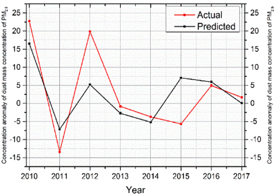 | ||
| Fig. 3 Prediction ability test of the linear regression equation for the anomaly of average dust surface mass concentration of PM2.5 for winter (from November to February) using the average of June and July Antarctic oscillation index (JJ–AAOI) from 2010 to 2017. | ||
Antarctic Oscillation Index (AAOI) and ice concentration
To gain further insight into the possible mechanism that may be the causative agent of this mechanism, the AAOI and the Antarctic sea ice were studied. The correlation results of the AAOI and the Antarctic sea ice concentration show that there is a significant correlation (at a 90% confidence level) between them even though the area, which shows a significant correlation, decreases as the lead–lag time increases (Fig. 4a–g). This is because the Antarctic sea ice distribution is significantly influenced by atmospheric pressure than other fields, such as temperature and wind.36,50–52 It is noteworthy that AAO is also defined based on GPH anomalies. However, the area exhibits significant correlation changes with the time of the year, i.e., each month shows different correlation results. The results from Fig. 4a and b suggest that August and September are the most significant months because large areas over the Antarctica region show a significant correlation during these two months.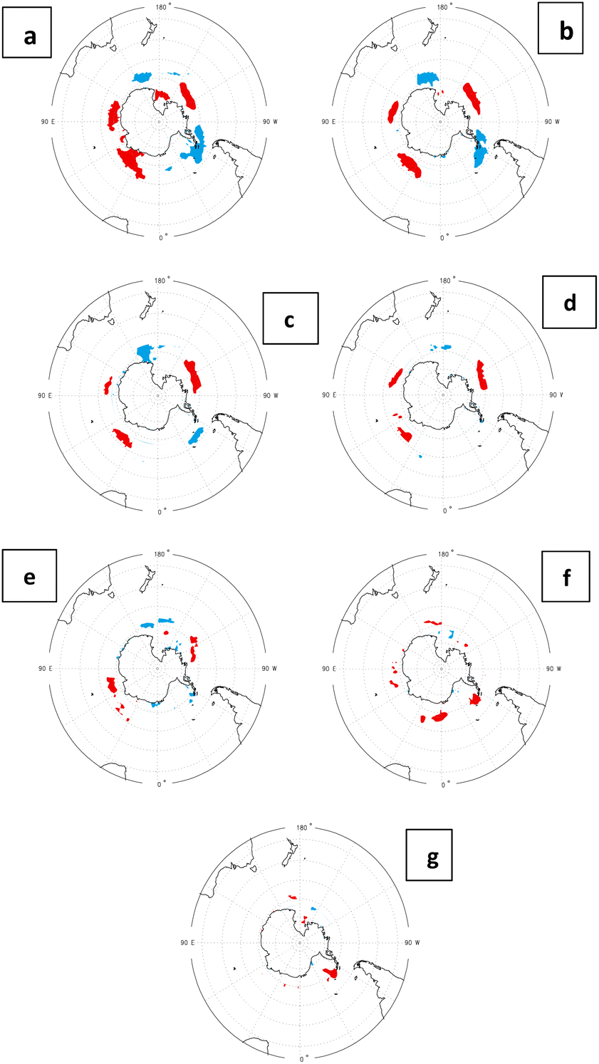 | ||
| Fig. 4 Correlation map between the average of June and July Antarctic oscillation index (JJ–AAOI) and the Antarctic sea ice over for the months of (a) August, (b) September, (c) October, (d) November, (e) December, (f) January, and (g) February for 36 years (i.e., from 1982 to 2017). The red (blue) color shows the area with a positive (negative) correlation with the JJ–AAOI at a 90% confidence level. | ||
Similarly, previous studies53,54 showed that the AAO signal normally tends to lead to climate anomalies by two to three months (one season). Likewise, a study by Carleton51 revealed that the indices (Southern Oscillation Index (SOI), Trans-Polar Index (TPI)) over SH lead the Antarctic sea ice for more than four months. The key areas identified during these two months of August and September were five (5): the first area was between 30 °E ∼50 °E and 59.5 °S ∼62 °S, the second area was between 90 °E ∼110 °E and 57.5 °S ∼61.5 °S, the third area was between 110 °E ∼170 °E and 61 °S ∼64 °S, the fourth area was between 110 °W ∼140 °W and 65 °S ∼68 °S, and the fifth area was between 40 °W ∼60 °W and 59 °S ∼65 °S. Similar areas of sea ice were determined in a study conducted by Wu and Zhang40 that significantly affected the atmosphere. The first, second and fourth key areas showed a positive correlation with AAOI, whereas the third and fifth areas showed a negative correlation. Interestingly, Fig. 4c and d show that during the austral spring season (October and November), the size of the areas, which showed a significant correlation (positive and negative), was reduced. The reduced areas indicate that the influence of the stored signals is reduced over time. Similarly, Fig. 4e–g shows the austral summer season (December, January, and February), in which the areas were further reduced and reached their minimum level at the end of February (Fig. 4g). Concurrent results to this have been reported by Gupta and England36 in their study of coupled ocean–atmosphere–ice response to variation in Southern Hemisphere Annular Mode (SAM) and by Hall and Visbeck52 in their study on the variability of SH sea ice from AAO. These findings suggest that the anomalies of the AAOI in June and July can be stored on Antarctic sea ice before it comes to influencing the ABLS, which, in the end, determines the distribution and concentration of dust surface mass concentrations of PM2.5 over East and North China. The signal of the AAOI can be imprinted and transmitted through an ice–sea–air system. Because the atmosphere cannot store long memories owing to the nature of atmospheric waves that are mostly chaotic,54–57 there is a need for a medium that can store this memory, such as sea ice. Therefore, the AAOI influences the boundary layer through the ice–sea–atmosphere interaction. A similar interaction of the ice–sea–atmosphere was revealed by Yuan and Li58 to be the most important interaction, which affects the atmospheric pressure and temperature. This lead–lag phenomenon is feasible because the observed atmospheric feedback mechanism is shorter than the atmospheric circulation of Rossby waves traveling from the Southern Hemisphere (SH) to the Northern Hemisphere (NH). A similar lead–lag time was reported by Shen and Mickley59 in the study of the effects of ENSO on summertime ozone pollution in the eastern United States. The subsection below uses the key areas of Antarctic sea ice to define a new ice index, aiming at quantifying the influence of ice concentration on dust surface mass concentration.
Ice index, AAOI, and pollutant distribution
To determine the weight contribution of different areas within the same month, a regression analysis was performed. Fig. 5 shows the weight contribution of five key areas, where the highest contribution was found to originate at 30 °E ∼ 50 °E and 59.5 °S ∼ 62 °S with a weight of eight-fold, while the lowest contribution originated at 40 °W ∼ 60 °W and 59 °S ∼ 65 °S with a contribution of negative three folds.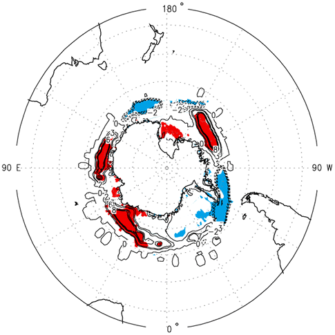 | ||
| Fig. 5 The average weight contribution of five key regions from August to October for 36 years (i.e., 1982 to 2017). The red (blue) color shows the area with the positive (negative) weight contribution of the key areas. | ||
This weighting contribution was used to develop the ice index that was then correlated with the AAOI; the correlation coefficient was found to be 0.6, and it was significant at a 99% confidence limit. The observed correlation is reasonable because AAOI tends to regulate sea ice through atmospheric, oceanic and dynamic forcing over the Antarctica area.36,50 Additionally, the difference in weight contribution suggests that the anomalies over the five correlated areas of Antarctica did not contribute equally to the observed trend of PM2.5 distribution. Moreover, the developed ice index showed a significant correlation at a 90% confidence limit with the dust surface mass concentration of PM2.5 around East and North China (figure not shown). These observed results imply that apart from other contributing factors, the Antarctic sea ice plays a key role in determining the distribution of pollutants over East and North China. At this juncture, one of the difficult questions that could arise is how does the dynamics over the Antarctic influence the pollutants on the other side of the hemisphere? One of the possible reasons that could be used to explain the occurrence of this mechanism is through the actions of wind. Furthermore, the correlation map of zonal and meridional winds with the ice index also showed a significant correlation over East and North China (Fig. 6).
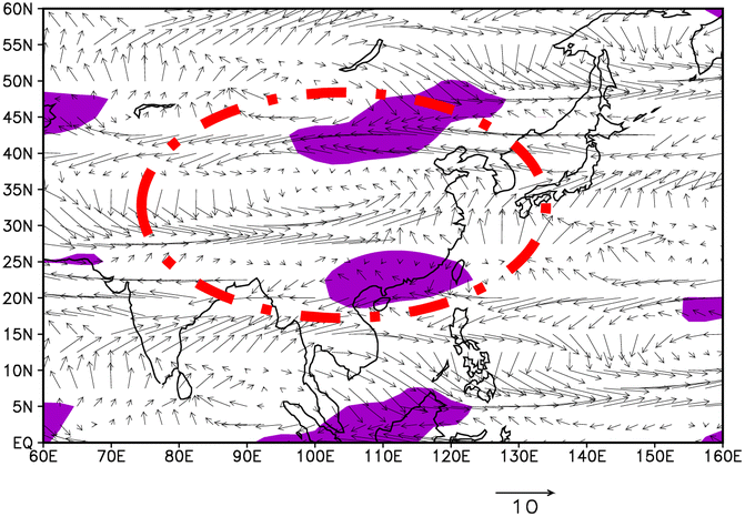 | ||
| Fig. 6 The correlation map between the average Antarctic Sea ice index of August to October and the average zonal and meridional wind (average of November to February) at 850 hPa from 1981–2018. The marked areas passed the significance correlation test at a 90% confidence level. | ||
Fig. 6 further shows that the eastern and northern parts of China acted as the center of the cyclone, which favors the accumulation of pollutants from the high-pressure zone. Therefore, this area acted as a convergence zone of pollutants from different areas. A similar observation was reported by Liang and Wang60 that East Asia Jetstream (EAJ) is the dominant wind field in China. In addition, a study by Zhang et al.61 associated a Rossby wave-like train in the mid-troposphere with haze pollution over northern China in December. Winds over this area originated from far areas, such as the northern part of India. Similarly, as presented in Fig. 6, this region is under the influence of southerly anomalies, resulting in a decline in clean and moist wind from the northern part. A previous study61 reveals the same scenario that vertical and horizontal movement of winds in this area was restricted by anomalous southerly wind, leading to a high period of haze days. Moreover, the stronger southerly and weaker northerly anomalies have been reported to weaken the East Asia winter monsoon.62 This condition is thought to generate stable atmospheric conditions, a favorable condition for pollutant accumulation. This observation indicates that the higher August to October sea ice index makes the southerly wind become stronger whereas the northerly wind becomes weaker. A similar observation was reported by several authors23,46 that higher August, September and October AAO (ASO–AAO) cause weaker northerly winds over North China. The effect of the North Atlantic Oscillation (NAO) cannot be neglected, as its large-scale climate variability model captures the Rossby wave train propagating downstream.63 The authors reveal that the negative phase of the preceding winter's NAO in northern China significantly affects the dust event at around 30 °N to 40 °N and 105 °E to 120 °E. Before the dust event, owing to the transient eddy momentum convergence over the dust aerosol source regions, the zonal wind speed increases in the upper-level troposphere, and the zonal wind in the middle–lower levels strengthens through momentum downward transmission.
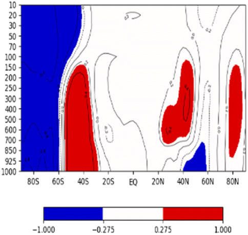
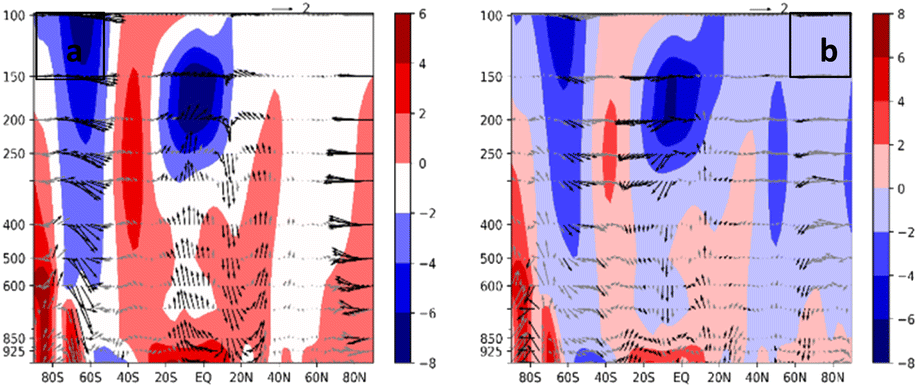
Fig. 7 depicts the latitude–altitude section for slopes of average zonal (80 °E − 130 °E) meridional wind over mainland China and the average of September and October AAOI (SO–AAOI). There is an AAO-like structure below the altitude of 850 hPa and positive anomalies at an altitude between 600 hPa and 70 hPa in SH at around 40 °S and 60 °S of the Equator (Fig. 7a). Over mainland China, there were positive anomalies below the altitude of 500 hPa with the center at around 850 hPa. At the equator, negative anomalies were observed below the altitude of 400 hPa. Similarly, the slope of the zonal wind shows an AAO-like structure between 40 °S and 60 °S throughout the troposphere, with the positive anomaly area extending to the stratosphere (Fig. 7b). Over the NH, there was a dipole-like structure ranging from 10 °N to 80 °N. As has been the case for zonal and meridional winds, the slopes of AAOI and GPH also show an AAO-like structure (Fig. 8) in the SH and a dipole-like structure in the NH. Positive anomalies over mainland China were found between the pressure levels of 700 hPa and 100 hPa. It is noteworthy that the dipole-like structure observed in NH was centered at around 200 hPa in almost all cases, i.e., it is the height of the dominant EAJ. As demonstrated by previous studies,60 EAJ is important in determining the weather conditions of mainland China.
 | ||
| Fig. 7 Latitude–altitude section for slopes of September and October Antarctic oscillation index (SO–AAOI) and mean zonal (80 °E − 130 °E) of (a) meridional (v) wind and (b) zonal (u) wind. The abscissa represents latitude, while the ordinate represents pressure levels. The marked area passed the significance test at a 90% confidence level. | ||
 | ||
| Fig. 8 Latitude–altitude section for slopes of September and October Antarctic oscillation index (SO–AAOI) and mean zonal (80 °E–130 °E) geopotential height. The abscissa represents latitude, while the ordinate represents pressure levels. The marked area passed the significance test at a 90% confidence level. | ||
These observed characteristics of the slope of AAOI with the GPH, zonal and meridional winds are clearly depicted in Fig. 6, showing the correlation map indicates that the most significant areas are between 20 °N and 50 °N as well as 100 °E and 125 °E. Therefore, this implies that the actions of winds and the influence of AAOI can potentially affect the distribution of pollutants in most parts of mainland China. Corroborated results have been reported by Fan and Wang21,45 studies on dust in North China, Zheng et al.54 study on the seasonal influence of AAOI on precipitation, and Wang and Fan64 study on the linkage between southern hemisphere zonal wind and East Asian summer monsoon circulation. In general, these studies indicate that the possible mechanism of the linkage between the Antarctic and NH is based mainly on meridional teleconnection.
Dust mass concentration and large-scale circulation
It is well established in the literature that large-scale circulation in both SH and NH affects the climate and weather patterns of China and Asia. To gain insight into the possible mechanism as to how climatic factors influence the distribution of pollutants over China, empirical orthogonal functions (EOFs) were used to decompose the variability of winter dust surface mass concentration of PM2.5 (November, December, January and February) from 1980 to 2018. As pointed out in the previous subsection, November is also included in the analysis because it was found to be highly polluted during the winter months. Therefore, its inclusion is necessary to capture the broader picture of what is happening during high pollutant periods. Fig. 9a and b show the first EOF (EOF1) and second EOF (EOF2) loadings of the dust mass surface concentrations of PM2.5, respectively. The EOF1 explains 40% of the original loading of the surface dust mass concentration of PM2.5 anomaly, which shows a swath of a positive anomaly over the northwest and eastern parts of China (Fig. 9a). A previous study by Bian et al.65 linked dust pollution in eastern China with this high-loading area identified by EOF1 in this area. The largest desert is in China: the Taklamakan and Gobi deserts. A study on the estimates of the ground concentration of PM2.5 based on satellite-derived aerosol optical depth by Ma et al.66 also indicated the Tarim Basin (i.e., Taklamakan desert) and Gobi desert similar to what has been identified by EOF1 as the potential sources of PM2.5 in China. It is therefore substantiated that these deserts can generate both coarse and fine particles, causing a high loading of PM2.5 dust mass concentration. It is noteworthy that the presence of deserts is not the only factor. For instance, a study conducted by Wang67 suggests that a high concentration of PM2.5 in northern China during winter is highly contributed to energy use, the effect of trade wind, and industrial emissions. A different scenario was observed on EOF2 that explains 29% of the total variance of dust mass concentration of PM2.5 because some parts of the central and northern area showed a negative correlation (Fig. 9b), that is, the area, which was identified to explain much of the loading by EOF1, showed a negative correlation in EOF2, which differs from what was reported in previous studies.65,66 This finding can be partially attributed to the small variance explained by EOF2 compared with that explained by EOF1. The maximum spatial loadings of EOF1 are found at 35 °N–42 °N and 75 °E–110 °E, and the average spatial loadings are found at around 22 °N–40 °N and 110 °E–125 °E. The time series of decomposed surface dust mass concentrations of PM2.5 for the leading principal component (PC1) and second principal component (PC2) are shown in Fig. 10a and b, respectively. Before 1992, the time series of PC1 showed a four-year wave train of negative and positive values (+, −, +) before it maintained the decadal negative value from 1997 to 2007. A different scenario was observed in the time series of PC2, as it showed a bi-decadal mode of negative values before 2000 and positive values after 2000, except in 2008 when it was negative. The values of PC2 post 2000 and 2009 have a time scale of eight and nine years of consecutive positive values, respectively. With due consideration of scant information from the variation trend of EOF2, this study does not consider EOF2 for further analysis. Therefore, this is suggested to provide an area of focus for other studies to further explore the possible association between EOF2 and the distribution of pollutants.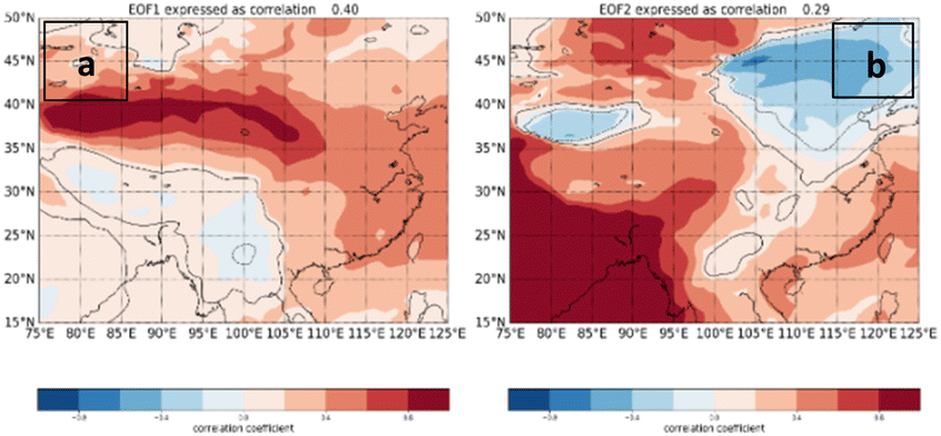 | ||
| Fig. 9 The loading of empirical orthogonal function (EOF) of average dust surface mass concentration of PM2.5 during the winter season (from November to February) from 1980 to 2018 across China: (a) EOF1 and (b) EOF2. | ||
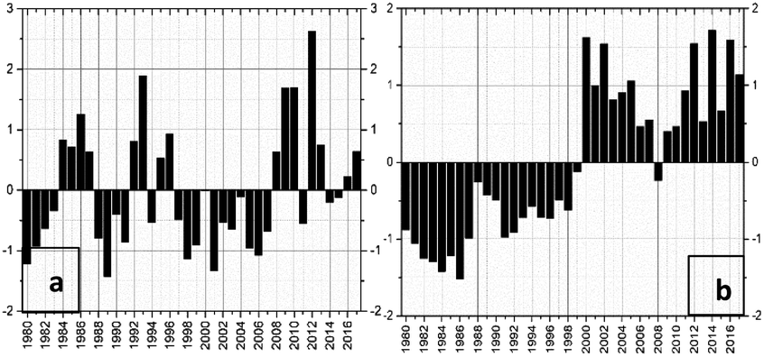 | ||
| Fig. 10 Normalized detrended time series of decomposed average dust surface mass concentration of PM2.5 during the winter season (from November to February) from 1980 to 2018: (a) leading principal component (PC1) and (b) second principal component (PC2). | ||
Because EOF1 explains much variance in dust mass concentrations of PM2.5 during winter (Fig. 10a), the correlation between climatic factors of boreal autumn (September and October) and PC1 was used to identify key areas with an influence on pollutant distribution in China. Fig. 11a shows the composite difference in meridional circulation between the years of high- and low-AAOI. The high and low years were selected after multiplying the standard deviation by 0.5 of the standardized JJ–AAOI. The years 1979, 1984, 1985, 1989, 1993, 1998, 2004, 2010, 2015, and 2016 were selected as the years of high positive JJ–AAOI, whereas the years 1991, 1992, 1996, 1997, 2005, 2007 and 2009 were selected as the years of low negative JJ–AAOI. Similarly, Fig. 11b shows the composite difference of meridional circulation between high and low PC1 year. The high and low years were also selected after multiplying the standard deviation by 0.5 of the standardized PC1. The years with positive high (negative low) PC1 were 1983, 1985, 1991, 1992, 1995, 2008, 2009, 2011, and 2012 (1979, 1980, 1988, 1990, 1997, 1998, 2000, 2004 and 2005). The shadings, which are seen on these figures (i.e., Fig. 10a and b), denote the climatology average of June and July vertical velocity (i.e., omega). A careful look at these figures shows ascending motions from the equator to around 40 °N and descending motion at around 60 °S and 20 °N. The observed intensification of the westerlies at around 60 °S and 75 °S during the high AAOI years has been reported in previous studies.32,52 Because the global meridional circulations in both SH and NH are connected and share ascending air mass branches, the meridional circulation changes in SH also affect the circulations in NH. The results from these figures show that significant ascending and southerly anomalies occur at around 25 °N and 35 °N during the positive JJ–AAOI years. Thus, the higher PC1 is concurrent with the overlaying ascending southerly anomaly, which is endorsed in one way or another by the positive phase of JJ–AAO. These observed scenarios during the positive phase of AAO are favorable for pollutant accumulation.
 | ||
| Fig. 11 Composite difference of September and October meridional circulation between high and low: (a) June and July AAOI years and (b) PC1. The shaded area represents the climatology vertical velocity (omega) with units of 1% Pa s−1 from 1980 to 2018, while the black vector represents the composite difference that reaches a 90% confidence level for the Student's t-test. | ||
Conclusions
The relationship between large-scale circulation and pollutant distribution was studied using a correlation map of AAOI and dust surface mass concentration of PM2.5 over mainland China. The area found to have a significant correlation was normalized and used to develop a time series of dust mass concentration. The correlation coefficient between the time series of dust mass concentration of PM2.5 and AAOI was 0.42: significant at the 95% confidence level. The lead–lag trend of the time series of pollutants and the JJ–AAOI was consistent except on two occasions (from 1988/89 to 1993/94 and 2013/14 to 2017/18). The inconsistency in these two occasions indicates that another prominent system was leading the AAO. Moreover, the highest and lowest AAOI years did not fall within these two occasions, which also supports the existence of other influencing systems, signifying that pollutant distribution does not depend on only one factor. Moreover, the JJ–AAOI was found to have a good correlation with the Antarctic sea ice concentration in the leading month over the key areas: 30 °E–50 °E and 59.5 °S–62 °S, 90 °E–110 °E and 57.5 °S–61.5 °S, 110 °E–170 °E and 61 °S–64 °S, 110 °W–140 °W and 65 °S–68 °S, and 40 °W–60 °W and 59 °S–65 °S. The correlation coefficient of the ice index developed from the regression analysis of the key areas with AAOI was 0.6, which was significant at 99%, indicating that the signals of AAOI are imprinted on Antarctic sea ice before they affect ABL and dust mass concentration. It is noteworthy that mainland China acts as the center of the cyclone (convergence zone). The persistence of the positive phase of J–AAO in NH was found to proceed up to December, in which the signals are transferred from higher latitudes to lower and mid-latitudes through the tropospheric vortex and the circumpolar westerlies. The cross-equatorial signal transfer is evident at pressure levels of 850 hPa and 500 hPa.Moreover, EOF1 was found to explain 40% of the total variability in the dust mass concentration of PM2.5 over mainland China. This is indicated by a swath of positive anomalies over the northeast, particularly over the Taklamakan and Gobi deserts, as well as the eastern part of the country. The maximum spatial loading of EOF1 is centered at around 35 °N–42 °N and 75 °E–110 °E as well as 22 °N–40 °N and 110 °E–125 °E; these areas are potential sources for dust mass before they find their way to the atmosphere through the action of winds. In contrast, EOF2, which explains 29% of the total variability, showed a negative correlation with dust mass concentration of PM2.5 over potential sources identified by EOF1, indicating that a different mechanism controls dust mass concentration. The EOF2 results could be partially attributed to their small variance. Furthermore, the time series of decomposed dust mass concentration of PM2.5 for PC1 revealed a four-year wave train of positive and negative values (+, −, +) before 1992 and the decadal negative train after the year 1997; the trend is concurrent with the calculated high and low years of PC1. The time series of PC2 indicates the existence of a bi-decadal mode of negative values before 2000 and a positive value after, except in 2008, in which there was a negative value. PC1 showed a significant zonally positive correlation with the zonal wind and negative tripole (+, −, +) pattern in the meridional direction. The positively correlated regions over mainland China were centered on the Taklamakan desert (40 °N and 95 °E), as was the case for the AAOI analysis. The zonally positive and negative patterns indicate that the zonal winds influenced the propagation of signals to mid-latitude. Moreover, the composite difference of meridional wind among the years of high and low June AAOI and the years of high and low PC1 showed that the significant ascending and southerly anomalies exhibit at around 25 °N and 35 °N during the years with high J–AAOI. It is noteworthy that this identified area falls within mainland China. Upon further research, the AAO and key areas identified over Antarctic sea ice can be used as the starting point for the effort to develop a comprehensive forecasting model for pollutant distribution in mainland China.
Conflicts of interest
There are no conflicts to declareReferences
- WHO, Ambient Air Pollution: A Global Assessment of Exposure and Burden of Diseases, Geneva, Switzerland, 2016 Search PubMed.
- WHO, 9 Out of 10 People Worldwide Breathe Polluted Air, but More Countries are Taking Action, https://www.who.int/news-room/detail/02-05-2018-9-out-of-10-people-worldwide-breathe-polluted-air-but-more-countries-are-taking-action Search PubMed.
- M. Li and L. Zhang, Haze in China: current and future challenges, Environ. Pollut., 2014, 189, 85–86 CrossRef CAS PubMed.
- X. P. Lyu, Z. W. Wang, H. R. Cheng, F. Zhang, G. Zhang, X. M. Wang, Z. H. Ling and N. Wang, Chemical characteristics of submicron particulates (PM1.0) in Wuhan, Central China, Atmos. Res., 2015, 161, 169–178 CrossRef.
- S. Han, J. Wu, Y. Zhang, Z. Cai, Y. Feng and Q. Yao, Characteristics and formation mechanism of a winter haze–fog episode in Tianjin, China, Atmos. Environ., 2014, 98, 323–330 CrossRef CAS.
- F. Yang, J. Tan, Q. Zhao, Z. Du, K. He, Y. Ma, F. Duan, G. Chen and Q. Zhao, Characteristics of PM2.5 speciation in representative megacities and across China, Atmos. Chem. Phys., 2011, 11, 5207–5219 CrossRef CAS.
- X. P. Lyu, N. Chen, H. Guo, L. Zeng, W. Zhang, F. Shen, J. Quan and N. Wang, Chemical characteristics and causes of airborne particulate pollution in warm seasons in Wuhan, central China, Atmos. Chem. Phys., 2016, 16, 10671–10687 CrossRef CAS.
- S. Wang, S. Yu, R. Yan, Q. Zhang, P. Li, L. Wang, W. Liu and X. Zheng, Characteristics and origins of air pollutants in Wuhan, China, based on observations and hybrid receptor models, J. Air Waste Manage. Assoc., 2016, 2247, 1240724, DOI:10.1080/10962247.2016.
- G. Xu, L. Jiao, B. Zhang, S. Zhao, M. Yuan, Y. Gu and J. Liu, Spatial and Temporal Variability of the PM2.5/PM10 Ratio in Wuhan, Central China, Aerosol Air Qual. Res., 2017, 17, 741–751 CrossRef CAS.
- Y. Mbululo, J. Qin and Z. Yuan, Boundary layer perspective assessment of air pollution status in Wuhan city from 2013 to 2017, Environ. Monit. Assess, 2019, 69(191), 1–12 Search PubMed.
- H. Zhao, H. Che, Y. Wang, Y. Dong, Y. Ma, X. Li, Y. Hong, H. Yang, Y. Liu, Y. Wang, K. Gui, T. Sun and Y. Zheng, Aerosol vertical distribution and typical air pollution episodes over North eastern China during 2016 analyzed by ground-based Lidar, Aerosol Air Qual. Res., 2018, 18, 918–937 CrossRef.
- N. Jiang, Z. Dong, Y. Xu, F. Yu, S. Yin, R. Zhang and X. Tang, Characterization of PM10 and PM2.5 Source Profiles of Fugitive Dust in Zhengzhou, China, Aerosol Air Qual. Res., 2018, 18, 314–329 CrossRef CAS.
- R. J. Huang, Y. Zhang, C. Bozzetti, K. F. Ho, J. J. Cao, Y. Han, K. R. Daellenbach, J. G. Slowik, S. M. Platt, F. Canonaco, P. Zotter, R. Wolf, S. M. Pieber, E. A. Bruns, M. Crippa, G. Ciarelli, A. Piazzalunga, M. Schwikowski, G. Abbaszade, J. Schnelle-Kreis, R. Zimmermann, Z. An, S. Szidat, U. Baltensperger, I. El Haddad and A. S. Prevot, High secondary aerosol contribution to particulate pollution during haze events in China, Nature, 2014, 514, 218–222 CrossRef CAS PubMed.
- Z. Song, D. Fu, X. Zhang, Y. Wu, X. Xia, J. He, X. Han, R. Zhang and H. Che, Diurnal and Seasonal Variability of PM2.5 and AOD in North China Plain: Comparison of MERRA-2 Products and Ground Measurements, Atmos. Environ., 2018, 191, 70–78 CrossRef CAS.
- X. M. Hu, Z. Ma, W. Lin, H. Zhang, J. Hu, Y. Wang, X. Xu, J. D. Fuentes and M. Xue, Impact of the Loess Plateau on the atmospheric boundary layer structure and air quality in the North China Plain: a case study, Sci. Total Environ., 2014, 499, 228–237 CrossRef CAS PubMed.
- Y. Mbululo, J. Qin and Z. Yuan, Evolution of atmospheric boundary layer structure and its relationship with air quality in Wuhan, China, Arabian J. Geosci., 2017, 10, 1–12 CrossRef CAS.
- Y. Mbululo, J. Qin, Z. Yuan, F. Nyihirani and X. Zheng, Boundary layer perspective assessment of air pollution status in Wuhan city from 2013 to 2017, Environ. Monit. Assess., 2019, 69(191), 1–12 Search PubMed.
- M. Wu, D. Wu, Q. Fan, B. M. Wang, H. W. Li and S. J. Fan, Observational studies of the meteorological characteristics associated with poor air quality over the Pearl River Delta in China, Atmos. Chem. Phys., 2013, 13, 10755–10766 CrossRef.
- Z. Yuan, J. Qin, X. Zheng and Y. Mbululo, The relationship between atmospheric circulation, boundary layer and near-surface turbulence in severe fog-haze pollution periods, J. Atmos. Sol.-Terr. Phys., 2020, 200, 105216 CrossRef.
- X. Zheng, J. Qin, S. Liang, Z. Yuan and Y. Mbululo, The Development of Boundary Layer Structure Index (BLSI) and Its Relationship with Ground Air Quality, Atmosphere, 2019, 10(3), 1–21 CrossRef.
- K. Fan and H. Wang, Dust storms in North China in 2002: a case study of the low frequency oscillation, Adv. Atmos. Sci., 2007, 24, 15–23 CrossRef.
- M. Gao, P. Sherman, S. Song, Y. Yu, Z. Wu and M. B. Mcelroy, Seasonal Prediction of Indian Wintertime Aerosol Pollution using the Ocean Memory Effect, Sci. Adv., 2019, 5, eaav4157 CrossRef CAS PubMed.
- Z. Zhang, D. Gong, R. Mao, L. Qiao, S. J. Kim and S. Liu, Possible Influence of the Antarctic Oscillation on Haze Pollution in North China, J. Geophys. Res.: Atmos., 2019, 124, 1307–1321 CrossRef.
- F. Zheng, J. Li, R. T. Clark, R. Ding, F. Li and L. Wang, Influence of the Boreal Spring Southern Annular Mode on Summer Surface Air Temperature over Northeast China, Atmos. Sci. Lett., 2015, 16, 155–161 CrossRef.
- E. Kalnay, M. Kanamitsu, R. Kistler, W. Collins, D. Deaven, L. Gandin, M. Iredell, S. Saha, G. White, J. Woollen, Y. Zhu, M. Chelliah, W. Ebisuzaki, W. Higgins, J. Janowiak, K. C. Mo, C. Ropelewski, J. Wang, A. Leetmaa, R. Reynolds, R. Jenne and D. Joseph, The NCEP/NCAR 40-year Reanalysis Project.pdf, Bull. Am. Meteorol. Soc., 1996, 77, 437–471 CrossRef.
- V. Buchard, C. A. Randles, A. M. da Silva, A. Darmenov, P. R. Colarco, R. Govindaraju, R. Ferrare, J. Hair, A. J. Beyersdorf, L. D. Ziemba and H. Yu, The MERRA-2 Aerosol Reanalysis, 1980 Onward. Part II: Evaluation and Case Studies, J. Clim., 2017, 30, 6851–6872 CrossRef CAS PubMed.
- L. He, A. Lin, X. Chen, H. Zhou, Z. Zhou and P. He, Assessment of MERRA-2 Surface PM2.5 over the Yangtze River Basin: ground-based verification, spatiotemporal distribution and meteorological dependence, Remote Sens., 2019, 11(4), 460 CrossRef.
- C. A. Randles, A. M. da Silva, V. Buchard, P. R. Colarco, A. Darmenov, R. Govindaraju, A. Smirnov, B. Holben, R. Ferrare, J. Hair, Y. Shinozuka and C. J. Flynn, The MERRA-2 Aerosol Reanalysis, 1980 Onward. Part I: System Description and Data Assimilation Evaluation, J. Clim., 2017, 30, 6823–6850 CrossRef CAS PubMed.
- R. Gelaro, W. McCarty, M. J. Suárez, R. Todling, A. Molod, L. Takacs, C. A. Randles, A. Darmenov, M. G. Bosilovich, R. Reichle, K. Wargan, L. Coy, R. Cullather, C. Draper, S. Akella, V. Buchard, A. Conaty, A. M. da Silva, W. Gu, G. K. Kim, R. Koster, R. Lucchesi, D. Merkova, J. E. Nielsen, G. Partyka, S. Pawson, W. Putman, M. Rienecker, S. D. Schubert, M. Sienkiewicz and B. Zhao, The modern-era retrospective analysis for research and applications, version 2 (MERRA-2), J. Clim., 2017, 30, 5419–5454 CrossRef PubMed.
- K. C. Mo, Relationships between low-frequency variability in the Southern Hemisphere and sea surface temperature anomalies, J. Clim., 2000, 13, 3599–3610 CrossRef.
- C. H. Ho, J. H. Kim, H. S. Kim, C. H. Sui and D. Y. Gong, Possible Influence of the Antarctic Oscillation on Tropical Cyclone Activity in the Western North Pacific, J. Geophys. Res. Atmos., 2005, 110, 1–11 Search PubMed.
- T. Liu, J. Li and F. Zheng, Influence of the Boreal Autumn Southern Annular Mode on Winter Precipitation over Land in the Northern Hemisphere, J. Clim., 2015, 28, 8825–8839 CrossRef.
- R. Mao, D. Y. Gong, J. Yang, Z. Y. Zhang, S. J. Kim and H. Z. He, Is there a linkage between the tropical cyclone activity in the southern Indian Ocean and the Antarctic Oscillation?, J. Geophys. Res.: Atmos., 2013, 118, 8519–8535 CrossRef.
- G. E. Silvestri and C. S. Vera, Antarctic Oscillation signal on precipitation anomalies over southeastern South America, Geophys. Res. Lett., 2003, 30, 1–4 CrossRef.
- G. J. Marshall, Trends in Antarctic geopotential height and temperature: a comparison between radiosonde and NCEP-NCAR reanalysis data, J. Clim., 2002, 15, 659–674 CrossRef.
- A. Sen Gupta and M. England, Coupled Ocean–Atmosphere–Ice Response to Variations in the Southern Annular Mode, J. Clim., 2006, 19, 4457–4486 CrossRef.
- J. Liu, X. Yuan, D. Rind and D. G. Martinson, Mechanism Study of the ENSO and Southern High Latitude Climate Teleconnections, Geophys. Res. Lett., 2002, 29, 8–11 Search PubMed.
- C. S. Bretherton, C. Smith and J. M. Wallace, J. Clim., 1992, 5, 541–560 CrossRef.
- C. Hu, Q. Wu, S. Yang, Y. Yao, D. Chan, Z. Li and K. Deng, A Linkage Observed between Austral Autumn Antarctic Oscillation and Preceding Southern Ocean SST Anomalies, J. Clim., 2016, 29, 2109–2122 CrossRef.
- Q. Wu and X. Zhang, Observed Evidence of an Impact of the Antarctic Sea Ice Dipole on the Antarctic Oscillation, J. Clim., 2011, 24, 4508–4518 CrossRef.
- Z. Yuan, J. Qin, S. Li, S. Huang and Y. Mbululo, Impact of Spring AAO on Summertime Precipitation in the North China Part: Observational Analysis, Asia-Pac. J. Atmos. Sci., 2020, 57(1), 1–16 Search PubMed.
- L. Li, R. Zhang, M. Wen, J. Duan and Y. Qi, Effects of the Atmospheric Dynamic and Thermodynamic Fields on the Eastward Propagation of Tibetan Plateau Vortices, Tellus A: Dyn. Meteorol. Oceanogr., 2019, 71, 1–12 CrossRef.
- D. Gong and S. Wang, Definition of Antarctic Oscillation Index, Geophys. Res. Lett., 1999, 26, 459–462 CrossRef.
- D. W. J. Thompson and J. M. Wallace, Annular modes in the extratropical circulation. Part I: month-to-month variability, J. Clim., 2000, 13, 1018–1036 CrossRef.
- K. Fan and H. Wang, Antarctic Oscillation and the Dust Weather Frequency in North China, Geophys. Res. Lett., 2004, 31, 1–5 CrossRef.
- H. Chen and H. Wang, Haze Days in North China and the associated atmospheric circulations based on daily visibility data from 1960 to 2012, J. Geophys. Res.: Atmos., 2015, 120, 5895–5909 CrossRef.
- S. Prabakaran, P. Naveen Kumar and P. Sai Mani Tarun, Rainfall Prediction using Modified Linear Regression, ARPN J. Eng. Appl. Sci., 2017, 12, 3715–3718 Search PubMed.
- S. Hastenrath, J. Clim., 1988, 1, 298–304 CrossRef.
- R. S. Selvaraj and R. Aditya, Statistical Method of Predicting the Northeast Rainfall of Tamil Nadu, Univers. J. Environ. Res. Technol., 2011, 1, 557–559 Search PubMed.
- X. Yuan and C. Li, Climate modes in southern high latitudes and their impacts on Antarctic sea ice, J. Geophys. Res., 2008, 113, 1–13 CrossRef.
- A. M. Carleton, Antarctic Sea-ice Relationships with Indices of the Atmospheric Circulation of the Southern Hemisphere, Clim. Dyn., 1989, 3, 207–220 CrossRef.
- A. Hall and M. Visbeck, Synchronous Variability in the Southern Hemisphere Atmosphere, Sea Ice, and Ocean Resulting from the Annular Mode, J. Clim., 2004, 17, 2249–2254 CrossRef.
- Z. Fei, L. I. Jianping and L. I. U. Ting, Some Advances in Studies of the Climatic Impacts of the Southern Hemisphere Annular Mode, J. Meteorol. Res., 2014, 29(5), 820–835 Search PubMed.
- F. Zheng, J. Li, L. Wang, F. Xie and X. Li, Cross-seasonal Influence of the December–February Southern Hemisphere Annular Mode on March–May Meridional Circulation and Precipitation, J. Clim., 2015, 28(17), 6859–6881 CrossRef.
- B. Wang, R. Wu and X. Fu, Pacific–East Asian Teleconnection: How Does ENSO Affect East Asian Climate, J. Clim., 2000, 13, 1517–1536 CrossRef.
- S. He and H. Wang, Impact of the November/December Arctic Oscillation on the following January temperature in East Asia, J. Geophys. Res.: Atmos., 2013, 118, 12981–12998 CrossRef.
- Z. Wu, J. Li, B. Wang and X. Liu, Can the Southern Hemisphere annular mode affect China winter monsoon, J. Geophys. Res., 2009, 114, 1–11 CrossRef.
- X. Yuan and C. Li, Climate modes in southern high latitudes and their impacts on Antarctic sea ice, J. Geophys. Res.: Oceans, 2008, 113(6) DOI:10.1029/2006JC004067.
- L. Shen and L. J. Mickley, Seasonal prediction of US summertime ozone using statistical analysis of large scale climate patterns, Proc. Natl. Acad. Sci., 2017, 114, 2491–2496 CrossRef CAS PubMed.
- X. Z. Liang and W. C. Wang, Associations between China monsoon rainfall and tropospheric jets, Q. J. R. Meteorol. Soc., 1998, 124, 2597–2623 CrossRef.
- X. Zhang, Z. Yin, H. Wang and M. Duan, Monthly Variations of Atmospheric Circulations Associated with Haze Pollution in the Yangtze River Delta and North China, Adv. Atmos. Sci., 2021, 38, 569–580 CrossRef.
- G. Zhang, Y. Gao, W. Cai, L. R. Leung, S. Wang, B. Zhao and M. Wang, Seesaw Haze Pollution in North China Modulated by the Sub-seasonal Variability of Atmospheric Circulation, Atmos. Chem. Phys., 2019, 15, 565–576 CrossRef.
- Y. Li, F. Xu, J. Feng, M. Du, W. Song, C. Li and W. Zhao, Influence of the previous North Atlantic Oscillation (NAO) on the spring dust aerosols over North China, Atmos. Chem. Phys., 2023, 23, 6021–6042 CrossRef CAS.
- H. Wang and K. Fan, Southern Hemisphere mean zonal wind in upper troposphere and East Asian summer monsoon circulation, Chin. Sci. Bull., 2006, 51, 1508–1514 Search PubMed.
- H. Bian, X. Tie, J. Cao, Z. Ying, S. Han and Y. Xue, Analysis of a severe dust storm event over China: application of the WRF-dust model, Aerosol Air Qual. Res., 2011, 11, 419–428 CrossRef.
- Z. Ma, X. Hu, L. Huang, J. Bi and Y. Liu, Estimating Ground-level PM2.5 in China Using Satellite Remote Sensing, Environ. Sci. Technol., 2014, 48, 7436–7444 CrossRef CAS PubMed.
- J. Wang, M. Zhang, X. Bai, H. Tan, S. Li, J. Liu, R. Zhang, M. A. Wolters, X. Qin, M. Zhang, H. Lin, Y. Li, J. Li and L. Chen, Large-scale transport of PM2.5 in the lower troposphere during winter cold surges in China, Sci. Rep., 2017, 7, 1–10 CrossRef PubMed.
| This journal is © The Royal Society of Chemistry 2023 |