
 Open Access Article
 This Open Access Article is licensed under a Creative Commons Attribution-Non Commercial 3.0 Unported Licence
Large-scale measurement of soil organic carbon using compact near-infrared spectrophotometers: effect of soil sample preparation and the use of local modelling†
Aymbiré A.
Fonseca
 ab,
Celio
Pasquini
*b and
Emanuelle. M. B.
Soares
a
ab,
Celio
Pasquini
*b and
Emanuelle. M. B.
Soares
a
aSoil Department, Federal University of Viçosa, Viçosa, Minas Gerais, Brazil
bChemistry Institute, University of Campinas, Campinas, São Paulo, Brazil. E-mail: pasquini@unicamp.br
First published on 31st July 2023
Abstract
Compact near-infrared (NIR) spectrophotometers are low-cost instruments that enable rapid, non-destructive and environmentally friendly measurement of soil organic carbon (SOC). However, several aspects, such as soil sample preparation modes or modelling strategies, related to the use of these instruments in large and heterogeneous data sets are yet to be addressed extensively. This work aimed to evaluate the performance of two compact NIR spectrophotometers (NeoSpectra and NanoNIR) to determine SOC content in a large-scale application. Also, it is important to understand the implications of soil sample preparation (soil grinding and drying) and the use of local partial least squares regression (LOCAL-PLSR) on the accuracy of the models built using these instruments. The soil samples of the calibration (n = 320, selected using the Kennard–Stone algorithm) and validation sets (n = 160) were collected from Minas Gerais state (approximately 589![[thin space (1/6-em)]](https://www.rsc.org/images/entities/char_2009.gif) 000 km2), Brazil. Three soil sample preparation modes were considered: air-dried and 2 mm sieved samples, air-dried and finely ground samples, and oven-dried and ground samples. Models to determine SOC were developed using the traditional PLSR (GLOBAL-PLSR) and a new approach based on LOCAL-PLSR, and their performance was evaluated using the root mean square error of prediction (RMSEP). The accuracy of the models built using the compact instruments was compared with the accuracy achieved using a bench Vis-NIR spectrophotometer. The NeoSpectra was the best-performing spectrophotometer, showing values of RMSEP, R2 and bias, respectively, between 5.2 and 6.3 g kg−1, 0.522 and 0.645 and −0.08 and −0.594. Significant enhancements in SOC estimation of up to 13% were found when models were calibrated using LOCAL-PLSR and oven-dried and ground soil samples. Our results showed that compact NIR spectrophotometers are a cost-effective alternative to the Vis-NIR spectrophotometers for large-scale SOC measurement. Models built using these instruments were accurate, mainly when LOCAL-PLSR calibration was used together with oven-dried and ground soil samples.
000 km2), Brazil. Three soil sample preparation modes were considered: air-dried and 2 mm sieved samples, air-dried and finely ground samples, and oven-dried and ground samples. Models to determine SOC were developed using the traditional PLSR (GLOBAL-PLSR) and a new approach based on LOCAL-PLSR, and their performance was evaluated using the root mean square error of prediction (RMSEP). The accuracy of the models built using the compact instruments was compared with the accuracy achieved using a bench Vis-NIR spectrophotometer. The NeoSpectra was the best-performing spectrophotometer, showing values of RMSEP, R2 and bias, respectively, between 5.2 and 6.3 g kg−1, 0.522 and 0.645 and −0.08 and −0.594. Significant enhancements in SOC estimation of up to 13% were found when models were calibrated using LOCAL-PLSR and oven-dried and ground soil samples. Our results showed that compact NIR spectrophotometers are a cost-effective alternative to the Vis-NIR spectrophotometers for large-scale SOC measurement. Models built using these instruments were accurate, mainly when LOCAL-PLSR calibration was used together with oven-dried and ground soil samples.
Environmental significanceIncreasing soil organic carbon (SOC) stocks are crucial to improve plant production systems and to mitigate global climate change, among other things. However, it is estimated that monitoring SOC has been generating more than 67000000 L per year of toxic acidic waste containing chromium globally, which poses a risk to human health. In contrast, near-infrared (NIR) spectroscopy is an environment-friendly technique that follows the green chemistry principles. Here we used compact NIR spectrophotometers to measure SOC on a large scale. Focus was given to the methodological aspects of using these instruments. Our results revealed that compact NIR spectrophotometers are a cost-effective alternative for large-scale SOC determination. Local modelling and soil sample preparation are strategies that can improve the performance of compact NIR spectrophotometers in the large-scale determination of SOC.
|
1. Introduction
Increasing soil organic carbon (SOC) levels can benefit several ecosystem services provided by soil, such as carbon sequestration and food production.1,2 However, managing soil to increase SOC requires well-substantiated knowledge of spatial and temporal behaviour of this attribute, which in turn requires characterizing it more extensively. More than 75% of soil analysis laboratories use wet oxidation proposed by Walkley–Black3 to determine SOC.4 Although wet oxidation is cheaper than dry oxidation (reference method), the method is laborious, time-consuming, and generates toxic acidic waste containing chromium.5 Considering the potential of 600 million soil samples to be analyzed globally,6 more than 67000000 L per year (approximately 150 mL per sample) of toxic waste can be generated by routine laboratories to determine SOC. It is therefore of particular importance to developing analytical methods to measure SOC content quickly, at low cost, without generating waste, which can be used in large-scale applications such as routine laboratory and precision agriculture.
In recent years, visible-near-infrared (Vis-NIR) spectroscopy has shown great potential for being implemented in soil analysis laboratories to determine SOC.4,7–10 This spectroscopic technique is fast, non-destructive, highly reproducible, and environmentally friendly, and has low operating costs. However, buying a Vis-NIR spectrophotometer remains rather expensive (usually higher than US $50000.00), mainly for small laboratories. Given recent technological advances in the last decade, several compact near-infrared (NIR) spectrophotometers are available nowadays.11,12 These instruments are usually small in size, light, and inexpensive (usually below US $5000.00), allowing their widespread application in soil analysis in small laboratories. When compared to Vis-NIR spectrophotometers, compact NIR instruments operate in a shorter range of the electromagnetic spectrum,11–13 but in terms of performance in SOC determination, the current literature shows that models based on these instruments can present excellent accuracy.10,14–16 However, the performance of compact NIR spectrophotometers in SOC determination using large and heterogeneous data sets has seldom been studied17 and, until now, methodological aspects such as soil sample preparation for using these instruments have not yet been addressed extensively.
One of the advantages of using diffuse reflectance spectroscopy to determine SOC is the possibility of measuring this attribute using 2 mm sieved soil samples.18 So, this is the most common soil sample preparation mode used in studies with compact NIR spectrophotometers in soil science (Table 1). However, even in a 2 mm sieved soil sample, the great diversity of particles with different origins, morphologies and granulometries can affect the representativeness of its spectrum, which in turn affect the performance of the models developed to estimate SOC.16 Previous research with Vis-NIR spectrophotometers has shown that these variabilities can be reduced by soil sample preparation before spectrum acquisition.19–21 Soil grinding increases the homogeneity of the sample particles, while soil drying reduces water dominance in the NIR spectra.19–21 Thus, these procedures may provide essential improvements to the performance of compact NIR spectrophotometers, especially considering that one of the most limiting aspects associated with these instruments is their smaller probing optical window.22
| Soil attributea | Multivariate methodb | Soil sample preparation | Source |
|---|---|---|---|
| a SOC = soil organic carbon; TN = total nitrogen, and TC = total carbon. b PLSR = partial least squares regression; RF = randon forest, CB = cubist, and SVM = support vector machine. | |||
| Routine soil analysis | PLSR | Oven-dried (40 °C) and 2 mm sieved | Soriano-Disla et al.33 |
| SOC, TN, pH | PLSR | Air-dried and 2 mm sieved | Ahmad Jani et al.15 |
| SOC, TN | PLSR | Oven-dried (40 °C) and 0.2 mm sieved | Barthès et al.14 |
| SOC, clay | PLSR/RF | Air-dried and 2 mm sieved | Karyotis et al.34 |
| SOC, TN | PLSR | Oven-dried (40 °C) and 2 mm sieved | Mura et al.10 |
| Cyanide | PLSR | Air-dried and 2 mm sieved | Sut et al.35 |
| SOC, TC | PLSR, CB, SVM | Air-dried and 2 mm sieved | Sharififar et al.17 |
Additionally, the partial least squares regression (GLOBAL-PLSR) is the most common multivariate method used to calibrate prediction models based on compact NIR spectrophotometers (Table 1). However, soil is a complex multicomponent matrix with several organic and inorganic compounds that absorb NIR radiation,23–26 so the use of databases composed of a wide diversity of soil types in terms of texture, mineralogy, parent material, and vegetation poses a challenge for modelling the spectral information related to SOC.27,28 Usually, increasing the scale of the data set makes it more complex, negatively affecting the accuracy of the models developed for SOC determination.4 An alternative approach for optimizing large spectral libraries is local modelling. The local partial least squares regression (LOCAL-PLSR) selects, from a large data set, a subset of samples spectrally similar to a given sample whose SOC content is to be predicted, reducing, in this way, spectral variabilities related to other soil attributes in the calibration set.29 Studies with Vis-NIR spectrophotometers have shown relevant improvements in the accuracy of models built from large spectral libraries when local modeling is used.30–32 Therefore, it is probable that this multivariate approach can also improve the performance of compact NIR spectrophotometers.
Considering the presented context, the main objectives of this work were to assess the performance of two compact NIR spectrophotometers in the large-scale measurement of SOC and to understand how the soil sample preparation and the use of local modeling can affect the performance of SOC determination models developed using this type of instrument. The results of the models built using compact spectrophotometers were compared to those of models based on the Vis-NIR spectrum.
2. Materials and methods
2.1. Study area and soil samples
The study was carried out using 523 soil samples collected from the Soil Bank of the state of Minas Gerais.36 The sampling points span an area of 589000 km2, covering all the main soil types found in Minas Gerais state, Brazil (Fig. 1). The soil samples were collected at a 0–20 cm depth in areas with preserved vegetation, located in different Brazilian biomes (Atlantic Forest, Caatinga, and Cerrado). After sample collection, the soil was air-dried, and sieved to 2 mm.
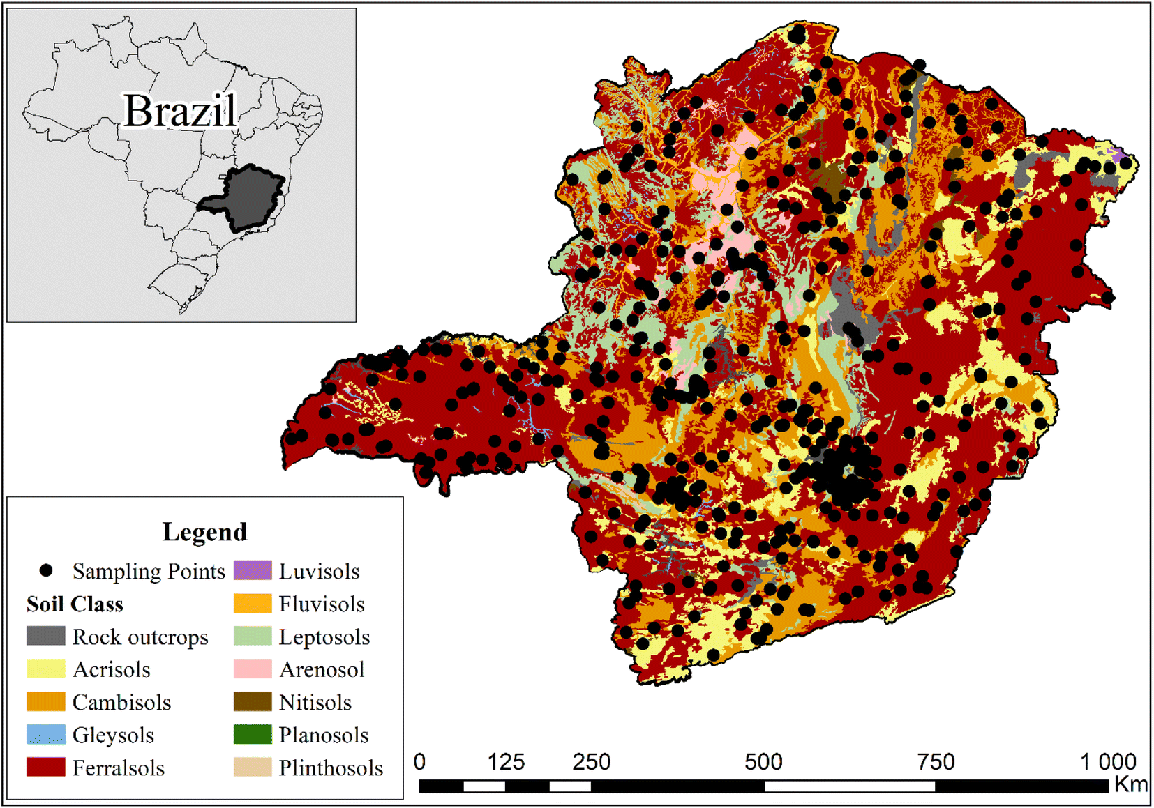 | ||
| Fig. 1 Collection locations and classes37 of the soil samples employed in this work. | ||
2.2. Reference analysis
The SOC content was measured using the Walkley–Black method.3 For this, 10 g subsamples of air-dried soil (<2 mm) were finely ground using a ball mill. Wet oxidation was performed using acidified potassium dichromate solution (K2Cr2O7 + H2SO4) as recommended.3 The SOC content varied from 0.6 g kg−1 to 44.7 g kg−1 (Fig. 2A).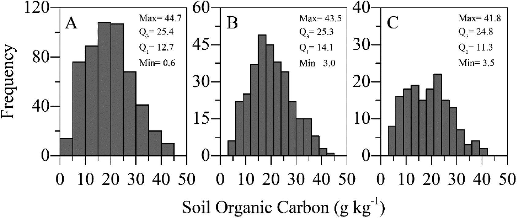 | ||
| Fig. 2 SOC contents as determined by the wet oxidation method and their occurring frequency observed for all data sets (A), in the calibration set (B), and the validation set (C). | ||
2.3. Spectral analysis
A rotation device was used to move the soil samples over the optical probing beam of these instruments during spectral data acquisition,16,22 increasing the representativeness of the spectral data. The soil samples were transferred to cylindrical glass vials with 20 mL volume (Sigma-Aldrich, Ref. DWK986541-500EA). During a measurement cycle (20 s – NeoSpectra; 21 s – NanoNIR), the vials were moved over the optical window of the spectrophotometers, performing six rotations. A complete description of the rotating sample device and its components can be found in Pasquini and Hespanhol (2021).22 In addition to providing better representative spectra, the rotational device minimizes the effect of ambient light on the instruments, as the flask containing the sample or Spectralon completely covers the probing window of the spectrophotometers during measurements.22
Spectrum acquisitions were made at the laboratory ambient temperature (25 ± 1 °C) considering that the effect of the temperature on the performance of the compact instruments has not been characterized yet.
The reflectance spectra (expressed in absorbance) were measured using the intensity of the signal obtained with a vial filled with Spectralon® as a reference for 100% reflectance. The compact spectrophotometers' spectrum acquisition protocol includes a reference measurement before each sample measurement.
To compare the performance of compact instruments in large-scale SOC against the performance obtained using Vis-NIR spectrophotometers, the same set of samples (composed of 523 soil samples) was scanned with a Fieldspec 3 spectroradiometer (Analytical Spectral Devices, ASD, Boulder, CO). This instrument operates in the 350–2500 nm range, with a spectral resolution of 1 nm from 350 to 700 nm, 3 nm from 700 to 1400 nm, and 10 nm from 1400 to 2500 nm.8 Spectral data from the Vis-NIR spectrophotometer were acquired by the GeoCiS group using oven-dried (45 °C) and 2 mm sieved soil samples as an average of 5 measured spectra taken at different locations on the sample.8 These spectra are part of the Brazilian Soil Spectral Library.8
All spectral transformations and pretreatments were performed using an Unscrambler X 10.4 (Camo, Norway).
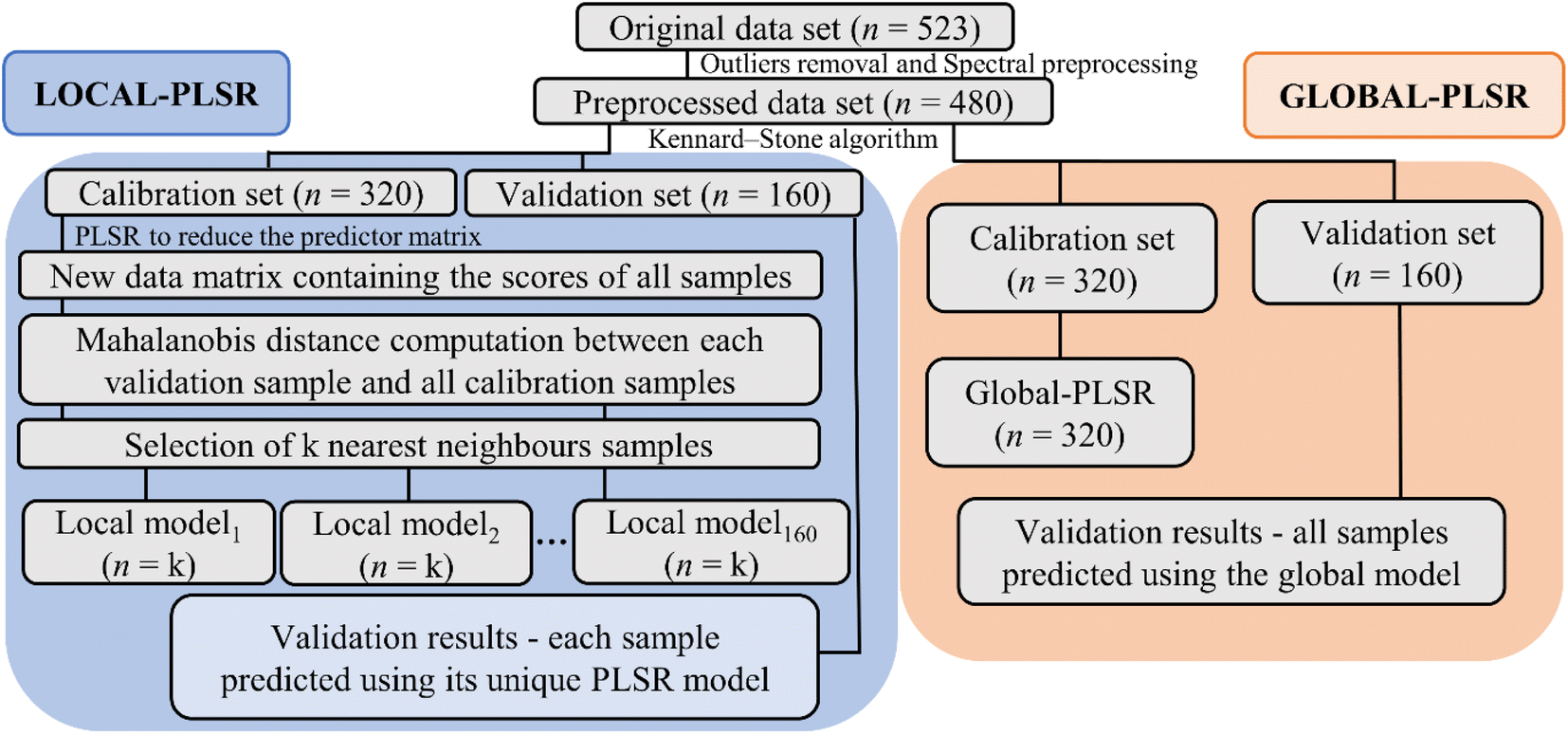 | ||
| Fig. 3 Flow chart of LOCAL-PLSR and GLOBAL-PLSR calibration procedures. For a given sample in the validation set, k is the number of nearest neighbor samples selected in the calibration set considering a given Mahalanobis limit distance. | ||
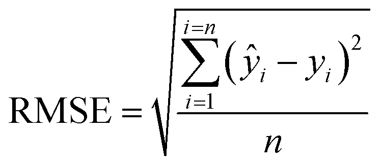
The optimal criterion to select the nearest neighbors to be included in the local calibration set has not yet been well established in the literature. Here, a code was implemented in the Jupyter Notebook interface with the Python language to select the best similarity criteria based on the Mahalanobis distance. Mahalanobis limit distances ranging from 0.1 to 3.5 (in steps of 0.1) were tested. After selecting the samples from the calibration set that satisfied the imposed similarity criterion, the LOCAL-PLSR models were constructed (Fig. 3) and the number of LV was optimized in each case by cross-validation and limited by the number of samples satisfying the distance criterion. The lower root means square error (RMSE) was employed to define the best Mahalanobis distance limit for each dataset (spectrophotometer type/sample preparation mode).
The main libraries used to build and evaluate the local models in the Jupyter Notebook interface were NumPy,41 Pandas,42 SciPy43 and Scikit-learn.44
3. Results
The absorbance and the first derivative spectra acquired using the NeoSpectra and NanoNIR and the different soil sample preparation modes are presented respectively in Fig. S1 and S2 of the ESI.† The spectrum set acquired using the bench Vis-NIR spectrophotometer is also presented in Fig. S1,† and their first-derivative spectra are in Fig. S2 (ESI).†3.1. Performance of compact spectrophotometers
Figures of merit of spectrophotometers' performance for GLOBAL-PLSR models are presented in Table 3, and the results of the randomization test for accuracy comparison among the models are presented in Table S1 of the ESI.† The NeoSpectra was the best-performing compact spectrophotometer for SOC prediction using GLOBAL-PLSR calibration (Tables 3 and S1 of the ESI†). The RMSEC of the models based on the NeoSpectra ranged from 5.4 to 5.7 g kg−1, values approximately 30% lower than that of the NanoNIR (Table 3). Additionally, the RPIQ values of the models built using the NeoSpectra were always greater than 2.0, as well as the one obtained with the Vis-NIR spectrophotometer (Table 3). The NeoSpectra was also the best-performing compact spectrophotometer to predict SOC in independent soil samples (Table 3). During the external validation procedure, the RMSEP of the models built using the NeoSpectra varied in the range of 6.0–6.3 g kg−1, values up to 12% lower than that obtained in the model developed using the Vis-NIR spectrophotometer (Tables 3 and S1 of the ESI†).| Spectrum acquisition protocol | Calibration | Independent validation | |||||
|---|---|---|---|---|---|---|---|
| LV | RMSEC (g kg−1) | R 2 | RPIQ | Bias | RMSEP (g kg−1) | ||
| a Mode I = air-dried and 2 mm sieved soil samples; Mode II = air-dried and ground soil samples; Mode III = oven-dried and ground soil samples. | |||||||
| NeoSpectra | Mode I | 10 | 5.7 | 0.522 | 2.0 | −0.08 | 6.3 |
| Mode II | 9 | 5.4 | 0.564 | 2.1 | −0.03 | 6.0 | |
| Mode III | 10 | 5.4 | 0.578 | 2.1 | −0.39 | 6.0 | |
| NanoNIR | Mode I | 2 | 7.6 | 0.151 | 1.5 | 1.05 | 8.2 |
| Mode II | 3 | 7.3 | 0.227 | 1.5 | 0.16 | 7.6 | |
| Mode III | 3 | 7.2 | 0.235 | 1.6 | 0.18 | 7.6 | |
| Vis-NIR | 9 | 5.5 | 0.549 | 2.0 | −0.01 | 6.8 | |
Models built using the NanoNIR showed worse accuracy (Table 3). Although the models built using this instrument required fewer latent variables to explain variations in SOC contents of the data set, probably as a function of the shorter spectral range covered by this instrument, their error of prediction was about 20% higher than that of the model developed using the Vis-NIR spectrophotometer (Tables 3 and S1 of the ESI†). In addition, the global models built using the NanoNIR presented RPIQ ≤ 1.5 and R2 ≤ 0.235 (Table 3).
Regardless of the SOC content in the soil samples, the results obtained with compact NIR spectrophotometers were highly repeatable. The mean values of SOC estimated from the ten spectra of the three analyzed samples employing the best local models were 15.8 ± 0.6, 21.8 ± 1.1 and 25.8 ± 1.5 g kg−1 when the NeoSpectra was used, and 14.1 ± 0.5, 20.0 ± 0.1 and 21.8 ± 0.1 g kg−1 when the NanoNIR was used. Therefore, the coefficient of variation of the results obtained with the compact instruments ranged from 0.5 to 5.9%. The reference values of SOC in these samples were, respectively, 12.9, 17.6 and 23.4 g kg−1.
3.2. Effect of soil sample preparation mode
The soil sample preparation mode affected the performance of the compact spectrophotometers in large-scale SOC determination (Tables 3 and S2 of the ESI†). Worse accuracy in both calibration and validation stages was obtained when air-dried and 2 mm sieved soil samples (Mode I) were used (Tables 3 and S2 of the ESI†). Using finely ground soil samples (Modes II and III) led to a reduction of 5.3% in RMSEC. It improved by up to 7.3% in model accuracy during the validation stage (Tables 3 and S2 of the ESI†). Additionally, models built using finely ground samples showed higher R2 and RPIQ than those built using the soil sample preparation Mode I (Table 3).Although grinding the soil has improved the performance of compact NIR spectrophotometers, the use of air-dried or oven-dried ground soil samples did not significantly (P value = 0.9) affect the performance of the NeoSpectra and NanoNIR in large-scale SOC determination (Tables 3 and S2 of the ESI†). Models built using soil sample preparation Modes I and II presented RMSEP = 6.0 g kg−1 when the NeoSpectra was used and RMSEP = 7.6 g kg−1 when the NanoNIR was used.
3.3. Effect of local modeling
Significant improvements in large-scale SOC determination were found using LOCAL-PLSR calibration (Tables 4 and S3 of the ESI†). The RMSEPs of the models built using the NeoSpectra ranged from 5.2 to 5.9 g kg−1, and those built using the NanoNIR ranged from 7.0 to 7.5 g kg−1 (Table 4). When minimal soil sample preparation was used (sample preparation Mode I), the RMSEP of the models built with the NeoSpectra reduced from 6.3 to 5.9 g kg−1, while those built with the NanoNIR reduced from 8.2 to 7.5 g kg−1. Thus, improvements of up to 9% in the performance of these instruments were provided by employing LOCAL-PLSR. Nevertheless, the most significant gain of using LOCAL-PLSR calibration occurred when soil sample preparation Modes II and III were used (Table 4). The RMSEP values of the LOCAL-PLSR were up to 15% lower than those obtained using GLOBAL-PLSR (Tables 4 and S3 of the ESI†) when finely ground soil samples were employed. The RPIQ values of the models calibrated using LOCAL-PLSR were higher than those of models built using GLOBAL-PLSR calibration, regardless of the compact spectrophotometer type and the soil sample preparation mode used (Table 4).| Instrument | Soil sample preparation | Independent validation | ||||
|---|---|---|---|---|---|---|
| Mahalanobis limit distance | RMSEP (g kg−1) | RPIQ | R 2 | Bias | ||
| a Mode I = air-dried and 2 mm sieved soil samples; Mode II = air-dried and ground soil samples; Mode III = oven-dried and ground soil samples. | ||||||
| NeoSpectra | Mode I | 2.6 | 5.9 | 2.3 | 0.534 | −0.594 |
| Mode II | 3.5 | 5.3 | 2.5 | 0.631 | −0.324 | |
| Mode III | 3.3 | 5.2 | 2.6 | 0.645 | −0.286 | |
| NanoNIR | Mode I | 1.4 | 7.5 | 1.8 | 0.247 | 0.305 |
| Mode II | 1.6 | 7.1 | 1.9 | 0.332 | −0.411 | |
| Mode III | 1.6 | 7.0 | 1.9 | 0.356 | −0.797 | |
4. Discussion
4.1. Spectrophotometer comparison
The NeoSpectra was the best-performing compact spectrophotometer in SOC determination. This performance appears to be related to the amount of information found over the more comprehensive NIR spectral range scanned using this instrument. The NanoNIR operates in the shorter wavelength range of 900–1700 nm. Although this region contains information regarding soil organic compounds, the spectral data obtained from it are generally related only to the second or third overtones of vibrational modes25,47,48 imparting lower sensitivity to the models. The NeoSpectra, in turn, operates in the range of 1350–2500 nm, and hence, the spectral data acquired using this instrument includes the combination absorption bands.25,47,48 Therefore, more information on the sample constituents is available for modeling using spectral data from the NeoSpectra. In this sense, it was expected that models based on Vis-NIR spectra would be the most accurate. However, this was not observed.It is known that SOC content changes the soil chroma, and these variations, in turn, affect the absorption intensity of electromagnetic radiation in the visible region, which could provide useful information for modeling SOC.4,8,48,49 However, the NeoSpectra performed better than the Vis-NIR spectrophotometer in determining SOC content in independent samples (validation set), although the accuracy achieved by the two instruments was similar for the calibration results. These results may be due to the representativeness of the spectral data acquired by each instrument. Compact spectrophotometers usually probe a smaller portion of the samples than conventional bench instruments, which may impair their performance.16,22 However, in this work these instruments were coupled to a rotation device, increasing the sample area exposed to the optical beam and improving their performance. The Vis-NIR bench instrument has no sample moving device and only 5 spectra were obtained at 5 locations on the sample to compose the average spectra used to construct the models. Furthermore, it is essential to understand that, although the NeoSpectra does not operate in the visible region, its spectra cover almost the entire NIR region. Therefore, the instrument provides information regarding organic species present in the samples with higher sensitivity found in the spectral region of the combination of vibrational modes (1900–2500 nm). This suffices to build accurate models to determine SOC, as can be depicted from the results presented in recent studies by Barthès et al. (2019);14 Beltrame et al. (2016);50 Fonseca et al. (2022);16 Soriano-Disla et al. (2017).33
4.2. Soil sample preparation mode
The RPmIQ of the GLOBAL-PLSR models built using NeoSpectra and the different soil sample preparation modes ranged from 2.0 to 2.1. This performance index is based on the RMSE of the model and the interquartile range of SOC in the soil population under study,45 and values between 2.0 and 2.5 indicate excellent quantitative models.45,51 Although the model built using soil sample preparation Mode I performed well, the accuracy of SOC prediction of the independent samples was higher employing finely ground soil samples. This improvement is due to the soil aggregate breakdown,19–21 which increases the homogeneity of the sample and the representativeness of the spectral data, improving their performance in SOC prediction.16The performance of the NanoNIR was also improved when the GLOBAL-PLSR was built using finely ground soil samples. However, even using the soil sample preparation Modes II and III, the highest RPIQ value achieved using this spectrophotometer was 1.6, indicating that the models performed poorly.45,51
In the current literature, no studies were found regarding the accuracy of compact NIR instruments aimed at SOC determination at a regional scale. Vis-NIR spectrophotometers have been studied for a longer time, and the average RMSEP value reported for regional models based on this instrument and minimally processed samples (air dry ≤ 2 mm soil samples) is 9.0 g kg−1.4 Models built with this kind of spectrophotometer and using a few soil types can be highly accurate, reaching RMSEP values of up to 1.3 g kg−1.16 However, the accuracy of SOC prediction decreases with the increasing scale of the dataset and the diversity of soils it contains.4,27,28 Note that the prediction errors obtained in the present work using the compact instruments were lower than 9.0 g kg−1, demonstrating the low-cost spectrophotometers' great potential.
4.3. Comparison between GLOBAL-PLSR and LOCAL-PLSR models
The performance of the compact spectrophotometers improved when LOCAL-PLSR calibration was used. The gain can be attributed to the reduction of spectral variabilities related to soil mineral composition found in the local calibration sets. In the NIR spectra of soils, the absorption bands associated with inorganic compounds are intense, prominent, and located in different wavelength regions according to the mineral composition.23 The absorption features associated with organic compounds are generally subtle and less intense and often superimposed with those of the mineral compounds.52 As GLOBAL-PLSR models calibrated on the large scale include several soil types, modeling the spectral information related to SOC is more complex, which impairs their performance.28 LOCAL-PLSR models, on the other hand, are calibrated using only those samples from the calibration set exhibiting the greatest spectral similarity and, consequently, mineral composition, with the measured sample. Thus, the variability of soil attributes and their effect on the spectra are reduced while the information related to SOC is evidenced and well located, improving the model's accuracy.28,53LOCAL-PLSR calibration is more cost-effective than grinding the sample to increase the accuracy of compact instruments for SOC determination. LOCAL-PLSR models built using minimal soil sample preparation were more accurate than GLOBAL-PLSR models, even when using laborious and energy-consuming ground soil samples. However, similarly to that observed for GLOBAL-PLSR models, increasing homogeneity by reducing particle size distribution through soil grinding (Barthès et al., 2006; Miltz and Don, 2012; Tamburini et al., 2017) further improves the performance of the LOCAL-PLSR models. As mentioned, the spectrum acquired from ground soil samples best represents its true composition. Therefore, when the spectral data of grinding soils are used to calibrate LOCAL-PLSR models, the selection of spectrally similar samples is more accurate, increasing the models' performance.
It is opportune to mention that the models developed using LOCAL-PLSR calibration can be even more accurate if more extensive spectral libraries are employed. The Mahalanobis distance threshold employed to select the nearest neighbors to be included in the local calibration set affects the performance of LOCAL-PLSR models (see Table S4 of the ESI†). When smaller Mahalanobis distances were used to select the samples with similar spectra to the evaluated sample (more restrictive similarity criteria), the RMSEP values were reduced to 2.8 g kg−1 (Table S4†). However, many samples from the validation set could not be assessed using the more restrictive criteria because the local calibration set could not be composed with enough samples to produce a reliable model. Thus, larger databases are needed to ensure the benefits of restrictive similarity criteria, as the calibration set needs a minimum number of similar samples to fit a model. The use of a more extensive spectral library, comprising about, for example, 10000 soil samples, may considerably improve the accuracy of LOCAL-PLSR models built with compact spectrophotometers.
On the other hand, extensive libraries are very costly. Therefore, instrument standardization needs to be provided sometime permitting large libraries to be transferred to several instruments of the same brand working in different laboratories. The current literature mentions several well succeeded studies reporting this relevant aspect of multivariate calibrations with compact instruments,54–57 conveying confidence that larger soil libraries could be also transferred. The continuity of this work will evaluate instrument standardization aiming for SOC determination.
5. Conclusion
The results of this work proved that compact NIR spectrophotometers are a cost-effective alternative to Vis-NIR spectrophotometers for large-scale SOC determination. The NeoSpectra (1350–2500 nm) was the best-performing spectrophotometer, delivering superior results compared to those of the Vis-NIR spectrophotometer. On the other hand, the use of the NanoNIR (900–1700 nm) resulted in models showing slightly lower accuracy for SOC prediction than the models obtained using the Vis-NIR spectrophotometer. However, using oven-dried and ground soil samples significantly improved the performance of both compact NIR spectrophotometers, especially when the models were calibrated using LOCAL-PLSR. Thus, this approach can make the use of the NanoNIR feasible.The LOCAL-PLSR calibration and grinding and drying of soil samples are strategies that increase the accuracy of compact NIR spectrophotometers in SOC determination. The best performance of the instruments was found when they were used together. Several soil spectral libraries have been built, and as far as we know, all of them are based on Vis-NIR spectra. These libraries are made up of a wide diversity of soil types. Our findings suggest that LOCAL-PLSR can be a better calibration tool than traditional GLOBAL-PLSR for determining SOC using these spectral libraries. However, the present spectral library is representative of the Brazilian state of Minas Gerais. Therefore, although the tested models performed well, they are limited by the representativeness currently covered by this library.
These achievements show the feasibility of expanding the use of NIR technology to aid environmental studies related to urgent issues about carbon sequestering and soil management. In addition, a study is underway to build the first Brazilian national soil spectral library based on compact spectrophotometers and propose a protocol for using this library in routine soil analysis laboratories.
Author contributions
A. A. Fonseca: conceptualization, methodology, formal analysis, investigation, software, data curation, writing-original draft and visualization. C. Pasquini: conceptualization, methodology, software, resources, writing – review & editing and supervision. E. M. B. Soares: conceptualization, methodology, investigation, resources, writing – review & editing, supervision, and project administration.Conflicts of interest
The authors declare that they have no known competing financial interests or personal relationships that could have appeared to influence the work reported in this paper.Acknowledgements
This work was supported by Coordenação de Aperfeiçoamento de Pessoal de Nível Superior – Brasil (CAPES) (Finance Code 001) and by Conselho Nacional de Desenvolvimento Científico e Tecnológico (CNPq) (Grants 465768/2014-8 (INCTAA) and 151343/2022-5). The authors gratefully acknowledge Dr José João Lelis Leal de Souza, Dr Walter Antônio Pereira Abrahão and Dr Reinaldo Bertola Cantarutti for providing the soil samples of the Soil Bank of the state of Minas Gerais, and the Instituto Nacional de Ciências e Tecnologias Analíticas Avançadas (INCTAA) for providing the spectrophotometers used in this study. The authors also acknowledge the Group GEOCIS (Geotecnologias em Ciência do Solo; Geotechnologies in Soil Science), https://esalqgeocis.wixsite.com/english, for the acquisition of the spectral dataset using a Vis-NIR spectrophotometer (FAPESP 2014-22262-0).References
- B. Minasny, B. P. Malone, A. B. McBratney, D. A. Angers, D. Arrouays, A. Chambers, V. Chaplot, Z. S. Chen, K. Cheng, B. S. Das, D. J. Field, A. Gimona, C. B. Hedley, S. Y. Hong, B. Mandal, B. P. Marchant, M. Martin, B. G. McConkey, V. L. Mulder, S. O'Rourke, A. C. Richer-de-Forges, I. Odeh, J. Padarian, K. Paustian, G. Pan, L. Poggio, I. Savin, V. Stolbovoy, U. Stockmann, Y. Sulaeman, C. C. Tsui, T. G. Vågen, B. van Wesemael and L. Winowiecki, Geoderma, 2017, 292, 59–86 CrossRef.
- E. K. Bünemann, G. Bongiorno, Z. Bai, R. E. Creamer, G. De Deyn, R. de Goede, L. Fleskens, V. Geissen, T. W. Kuyper, P. Mäder, M. Pulleman, W. Sukkel, J. W. van Groenigen and L. Brussaard, Soil Biol. Biochem., 2018, 120, 105–125 CrossRef.
- A. Walkley and I. A. Black, Soil Sci., 1934, 37, 29–38 CrossRef CAS.
- R. A. V. Rossel, T. Behrens, E. Ben-Dor, D. J. Brown, J. A. M. Demattê, K. D. Shepherd, Z. Shi, B. Stenberg, A. Stevens, V. Adamchuk, H. Aïchi, B. G. Barthès, H. M. Bartholomeus, A. D. Bayer, M. Bernoux, K. Böttcher, L. Brodský, C. W. Du, A. Chappell, Y. Fouad, V. Genot, C. Gomez, S. Grunwald, A. Gubler, C. Guerrero, C. B. Hedley, M. Knadel, H. J. M. Morrás, M. Nocita, L. Ramirez-Lopez, P. Roudier, E. M. R. Campos, P. Sanborn, V. M. Sellitto, K. A. Sudduth, B. G. Rawlins, C. Walter, L. A. Winowiecki, S. Y. Hong and W. Ji, Earth Sci. Rev., 2016, 155, 198–230 CrossRef.
- F. B. Santana, A. M. Souza and R. J. Poppi, Sci. Total Environ., 2019, 658, 895–900 CrossRef PubMed.
- J. A. M. Demattê, A. C. Dotto, L. G. Bedin, V. M. Sayão and A. B. e Souza, Geoderma, 2019, 337, 111–121 CrossRef.
- A. Ahmadi, M. Emami, A. Daccache and L. He, Agronomy, 2021, 11(3), 433 CrossRef CAS.
- J. A. M. Demattê, A. C. Dotto, A. F. S. Paiva, M. v. Sato, R. S. D. Dalmolin, M. d. S. B. de Araújo, E. B. da Silva, M. R. Nanni, A. ten Caten, N. C. Noronha, M. P. C. Lacerda, J. C. de Araújo Filho, R. Rizzo, H. Bellinaso, M. R. Francelino, C. E. G. R. Schaefer, L. E. Vicente, U. J. dos Santos, E. v. de Sá Barretto Sampaio, R. S. C. Menezes, J. J. L. L. de Souza, W. A. P. Abrahão, R. M. Coelho, C. R. Grego, J. L. Lani, A. R. Fernandes, D. A. M. Gonçalves, S. H. G. Silva, M. D. de Menezes, N. Curi, E. G. Couto, L. H. C. dos Anjos, M. B. Ceddia, É. F. M. Pinheiro, S. Grunwald, G. M. Vasques, J. Marques Júnior, A. J. da Silva, M. C. de V. Barreto, G. N. Nóbrega, M. Z. da Silva, S. F. de Souza, G. S. Valladares, J. H. M. Viana, F. da Silva Terra, I. Horák-Terra, P. R. Fiorio, R. C. da Silva, E. F. Frade Júnior, R. H. C. Lima, J. M. F. Alba, V. S. de Souza Junior, M. D. L. M. S. Brefin, M. D. L. P. Ruivo, T. O. Ferreira, M. A. Brait, N. R. Caetano, I. Bringhenti, W. de Sousa Mendes, J. L. Safanelli, C. C. B. Guimarães, R. R. Poppiel, A. B. e Souza, C. A. Quesada and H. T. Z. do Couto, Geoderma, 2019, 354, 113793 CrossRef.
- R. A. V. Rossel, T. Behrens, E. Ben-Dor, S. Chabrillat, J. A. M. Demattê, Y. Ge, C. Gomez, C. Guerrero, Y. Peng, L. Ramirez-Lopez, Z. Shi, B. Stenberg, R. Webster, L. Winowiecki and Z. Shen, Eur. J. Soil Sci., 2022, 73(4), e13271 Search PubMed.
- S. Mura, C. Cappai, G. F. Greppi, S. Barzaghi, A. Stellari and T. M. P. Cattaneo, Comput. Electron. Agric., 2019, 159, 92–96 CrossRef.
- C. Pasquini, Anal. Chim. Acta, 2018, 1026, 8–36 CrossRef CAS PubMed.
- K. B. Beć, J. Grabska, H. W. Siesler and C. W. Huck, NIR News, 2020, 31, 28–35 CrossRef.
- C. A. T. dos Santos, M. Lopo, R. N. M. J. Páscoa and J. A. Lopes, Appl. Spectrosc., 2013, 67, 1215–1233 CrossRef PubMed.
- B. G. Barthès, E. Kouakoua, M. Clairotte, J. Lallemand, L. Chapuis-Lardy, M. Rabenarivo and S. Roussel, Geoderma, 2019, 338, 422–429 CrossRef.
- H. F. Ahmad Jani, R. Meder, H. A. Hamid, S. M. Razali and K. H. M. Yusoff, J. Near Infrared Spectrosc., 2021, 29, 148–157 CrossRef CAS.
- A. A. da Fonseca, C. Pasquini, D. C. Costa and E. M. B. Soares, Geoderma, 2022, 409, 115636 CrossRef.
- A. Sharififar, K. Singh, E. Jones, F. I. Ginting and B. Minasny, Soil Use Manag., 2019, 35, 607–616 CrossRef.
- S. Li, R. A. V. Rossel and R. Webster, Eur. J. Soil Sci., 2021, 73(1), e13202 Search PubMed.
- E. Tamburini, F. Vincenzi, S. Costa, P. Mantovi, P. Pedrini and G. Castaldelli, Sensors, 2017, 17, 2366 CrossRef PubMed.
- B. G. Barthès, D. Brunet, H. Ferrer, J. L. Chotte and C. Feller, J. Near Infrared Spectrosc., 2006, 14, 341–348 CrossRef.
- J. Miltz and A. Don, J. Near Infrared Spectrosc., 2012, 20, 695–706 CrossRef CAS.
- C. Pasquini and M. C. Hespanhol, Microchem. J., 2021, 170, 106747 CrossRef CAS.
- Q. Fang, H. Hong, L. Zhao, S. Kukolich, K. Yin and C. Wang, J. Spectrosc., 2018, 2018, 1–14 CrossRef.
- B. Stenberg, R. A. V. Rossel, A. M. Mouazen and J. Wetterlind, in Advances in Agronomy, ed. D. L. Sparks, Academic Press, Burlington, 2010, vol. 107, pp. 163–215 Search PubMed.
- R. A. V. Rossel and T. Behrens, Geoderma, 2010, 158, 46–54 CrossRef CAS.
- J. Wetterlind, R. A. V. Rossel and M. Steffens, Eur. J. Soil Sci., 2022, 73(4), e13263 CrossRef CAS.
- Y. Hong, Y. Chen, Y. Zhang, Y. Liu, Y. Liu, L. Yu, Y. Liu and H. Cheng, Soil Sci. Soc. Am. J., 2018, 82, 1231–1242 CrossRef CAS.
- S. Liu, H. Shen, S. Chen, X. Zhao, A. Biswas, X. Jia, Z. Shi and J. Fang, Geoderma, 2019, 348, 37–44 CrossRef CAS.
- J. S. Shenk, M. O. Westerhaus and P. Berzaghi, J. Near Infrared Spectrosc., 1997, 5, 223–232 CrossRef CAS.
- F. Gogé, R. Joffre, C. Jolivet, I. Ross and L. Ranjard, Chemom. Intell. Lab. Syst., 2012, 110, 168–176 CrossRef.
- M. s. Luce, N. Ziadi and R. A. V. Rossel, Geoderma, 2022, 425, 116048 CrossRef.
- C. R. Lobsey, R. A. V. Rossel, P. Roudier and C. B. Hedley, Eur. J. Soil Sci., 2017, 68, 840–852 CrossRef CAS.
- J. M. Soriano-Disla, L. J. Janik, D. J. Allen and M. J. McLaughlin, Biosyst. Eng., 2017, 161, 24–36 CrossRef.
- K. Karyotis, T. Angelopoulou, N. Tziolas, E. Palaiologou, N. Samarinas and G. Zalidis, Land, 2021, 10, 63 CrossRef.
- M. Sut, T. Fischer, F. Repmann, T. Raab and T. Dimitrova, Water, Air, Soil Pollut., 2012, 223, 5495–5504 CrossRef CAS.
- J. J. L. L. de Souza, W. A. P. Abrahão, J. W. V. de Mello, J. da Silva, L. M. da Costa and T. S. de Oliveira, Sci. Total Environ., 2015, 505, 338–349 CrossRef CAS PubMed.
- UFV, UFOP, UFLA and CETEC, Mapa de Solos do Estado de Minas Gerais, Viçosa, 2010 Search PubMed.
- A. Savitzky and M. J. E. Golay, Anal. Chem., 1964, 36, 1627–1639 CrossRef CAS.
- R. W. Kennard and L. A. Stone, Technometrics, 1969, 11, 137–148 CrossRef.
- G. Shen, M. Lesnoff, V. Baeten, P. Dardenne, F. Davrieux, H. Ceballos, J. Belalcazar, D. Dufour, Z. Yang, L. Han, J. Antonio and F. Pierna, J. Chemom., 2019, 33(5), 1–3 CrossRef.
- C. R. Harris, K. J. Millman, S. J. van der Walt, R. Gommers, P. Virtanen, D. Cournapeau, E. Wieser, J. Taylor, S. Berg, N. J. Smith, R. Kern, M. Picus, S. Hoyer, M. H. van Kerkwijk, M. Brett, A. Haldane, J. F. del Río, M. Wiebe, P. Peterson, P. Gérard-Marchant, K. Sheppard, T. Reddy, W. Weckesser, H. Abbasi, C. Gohlke and T. E. Oliphant, Nature, 2020, 585, 357–362 CrossRef CAS PubMed.
- W. McKinney, Proceedings of the 9th Python in Science Conference, 2010, 1, pp. 56–61 Search PubMed.
- P. Virtanen, R. Gommers, T. E. Oliphant, M. Haberland, T. Reddy, D. Cournapeau, E. Burovski, P. Peterson, W. Weckesser, J. Bright, S. J. van der Walt, M. Brett, J. Wilson, K. J. Millman, N. Mayorov, A. R. J. Nelson, E. Jones, R. Kern, E. Larson, C. J. Carey, İ. Polat, Y. Feng, E. W. Moore, J. VanderPlas, D. Laxalde, J. Perktold, R. Cimrman, I. Henriksen, E. A. Quintero, C. R. Harris, A. M. Archibald, A. H. Ribeiro, F. Pedregosa, P. van Mulbregt, A. Vijaykumar, A. P. Bardelli, A. Rothberg, A. Hilboll, A. Kloeckner, A. Scopatz, A. Lee, A. Rokem, C. N. Woods, C. Fulton, C. Masson, C. Häggström, C. Fitzgerald, D. A. Nicholson, D. R. Hagen, D. V. Pasechnik, E. Olivetti, E. Martin, E. Wieser, F. Silva, F. Lenders, F. Wilhelm, G. Young, G. A. Price, G. L. Ingold, G. E. Allen, G. R. Lee, H. Audren, I. Probst, J. P. Dietrich, J. Silterra, J. T. Webber, J. Slavič, J. Nothman, J. Buchner, J. Kulick, J. L. Schönberger, J. V. de Miranda Cardoso, J. Reimer, J. Harrington, J. L. C. Rodríguez, J. Nunez-Iglesias, J. Kuczynski, K. Tritz, M. Thoma, M. Newville, M. Kümmerer, M. Bolingbroke, M. Tartre, M. Pak, N. J. Smith, N. Nowaczyk, N. Shebanov, O. Pavlyk, P. A. Brodtkorb, P. Lee, R. T. McGibbon, R. Feldbauer, S. Lewis, S. Tygier, S. Sievert, S. Vigna, S. Peterson, S. More, T. Pudlik, T. Oshima, T. J. Pingel, T. P. Robitaille, T. Spura, T. R. Jones, T. Cera, T. Leslie, T. Zito, T. Krauss, U. Upadhyay, Y. O. Halchenko and Y. Vázquez-Baeza, Nat. Methods, 2020, 17, 261–272 CrossRef CAS PubMed.
- F. Pedregosa, G. Varoquaux, A. Gramfort, V. Michel, B. Thirion, O. Grisel, M. Blondel, P. Prettenhofer, R. Weiss, V. Dubourg, J. Vanderplas, A. Passos, D. Cournapeau, M. Brucher, M. Perrot and É. Duchesnay, J. Mach. Learn. Res., 2011, 12, 2825–2830 Search PubMed.
- V. Bellon-Maurel, E. Fernandez-Ahumada, B. Palagos, J. M. Roger and A. McBratney, TrAC, Trends Anal. Chem., 2010, 29, 1073–1081 CrossRef CAS.
- A. C. Olivieri, Introduction to Multivariate Calibration, Springer International Publishing, Cham, 2018 Search PubMed.
- J. Workman and L. Weyer, Practical Guide to Interpretive Near-Infrared Spectroscopy, Taylor & Francis Group, Boca Raton, 2008 Search PubMed.
- B. Stenberg, R. A. V. Rossel, A. M. Mouazen and J. Wetterlind, Visible and Near Infrared Spectroscopy in Soil Science, 2010, vol. 107 Search PubMed.
- M. P. C. Lacerda, J. A. M. Demattê, M. v. Sato, C. T. Fongaro, B. C. Gallo and A. B. Souza, Remote Sens., 2016, 8(9), 701 CrossRef.
- K. K. Beltrame, A. M. Souza, M. R. Coelho, T. C. B. Winkler, W. E. Souza and P. Valderrama, J. Braz. Chem. Soc., 2016, 27, 1527–1532 CAS.
- A. P. Leone, R. A. Viscarra-Rossel, P. Amenta and A. Buondonno, Curr. Anal. Chem., 2012, 8, 283–299 CrossRef CAS.
- R. A. V. Rossel, A. Chappell, P. De Caritat and N. J. Mckenzie, Eur. J. Soil Sci., 2011, 62, 442–453 CrossRef.
- Z. Shi, W. Ji, R. A. V. Rossel, S. Chen and Y. Zhou, Eur. J. Soil Sci., 2015, 66, 679–687 CrossRef CAS.
- N. C. da Silva, C. J. Cavalcanti, F. A. Honorato, J. M. Amigo and M. F. Pimentel, Anal. Chim. Acta, 2017, 954, 32–42 CrossRef PubMed.
- L. Li, W. Huang, Z. Wang, S. Liu, X. He and S. Fan, Postharvest Biol. Technol., 2022, 183, 111720 CrossRef CAS.
- X. Li, S. Arzhantsev, J. F. Kauffman and J. A. Spencer, J. Pharm. Biomed. Anal., 2011, 54, 1001–1006 CrossRef CAS PubMed.
- M. Eady, M. Payne, C. Changpim, M. Jinnah, S. Sortijas and D. Jenkins, Spectrochim. Acta, Part A, 2022, 267, 120512 CrossRef CAS PubMed.
Footnote |
| † Electronic supplementary information (ESI) available. See DOI: https://doi.org/10.1039/d3va00046j |
| This journal is © The Royal Society of Chemistry 2023 |