Does the accounting of the local symmetry fragments in SMILES improve the predictive potential of the QSPR-model for Henry's law constants?†
Received
18th January 2023
, Accepted 5th May 2023
First published on 8th May 2023
Abstract
When modeling many physicochemical, biochemical, and ecological processes, numerical data on Henry's law constants are much desired. In addition, these data are used in pharmaceuticals for the development of gaseous drugs, as well as in modeling drug–receptor interactions. Henry's law constant is an indicator of the affinity of compounds for the vapor phase and water. The local symmetry of simplified molecular input-line entry systems (SMILES) comprises compositions of identical symbols that can be represented as three ‘xyx’, four ‘xyyx’, or five symbols ‘xyzyx’. Taking account of these attributes of SMILES can improve the predictive potential of models for Henry's law constants. We updated our CORAL software using the optimal (flexible) descriptor. The updated descriptor improved the predictive potential when applied to the model for Henry's law constants. This new approach also permits fast definition of a set of pollutants that have a minimal impact on climate change and are safe from an environmental point of view.
Environmental significance
Computational support for usual experiments is a necessary element of research work. In order to improve the environmental situation in the atmosphere, data on Henry's law constants are needed for currently used and new substances. Reliable computer prediction of the mentioned constants is a problem solved by means of numerous approaches. The approach proposed here is economical and convenient for quickly evaluating large lists of organic molecules. The possibility of taking into account the influence of local symmetry is an attractive feature and an important advantage of the approach under consideration since it has both a heuristic and general theoretical orientation.
|
1. Introduction
Chemical changes in aerosols affect the fate of atmospheric pollutants and ecology, climate, and human health-relevant aerosol properties. The constants of Henry's law are useful for assessing the processes related to atmospheric pollutants, particularly those related to their transport in the atmosphere. However, at present experimental values of the constants of Henry's law are only available for some compounds. Instrumental problems, detection limits of low concentrations of hydrophobic compounds, and other factors make the experimental determination of the constants of Henry's law difficult and expensive.1,2
In the last few years, quantitative structure–property relationship (QSPR) models have become a popular, inexpensive and rapid tool for predicting different compounds' physicochemical and biochemical behavior.1–5 Henry's law constants have also been studied in the literature.6–10 One of the variants of QSPR analysis focused on the representation of the molecular structure by means of SMILES strings,11 followed by the Monte Carlo determination of the correlation weights for various fragments of the SMILES strings12–14 using CORAL software (http://www.insilico.eu/coral). The present study aims to develop a QSPR model for Henry's law constants using the updated list of SMILES attributes involved in Monte Carlo calculations referred to as the fragments of the local symmetry.
2. Method
2.1 Data
Experimental data on Henry's law constants at 25 °C ([atm m3 mol−1] expressed in decimal logarithms were taken from the literature.2 The source contains 530 heterogeneous compounds which includes pesticides, solvents, aromatic hydrocarbons and persistent pollutants, but the CORAL program (http://www.insilico.eu/coral) detected three duplicates (Table S1, ESI†). Therefore, 527 compounds were used to build up QSPR models. Here, three random splits into active training, passive training, calibration and validation sets are studied.
2.2 Optimal descriptor
The optimal descriptor applied here is calculated as:| | | DCW(T,N) = ∑CW(Sk) + ∑CW(SSk) + CW(xyx) + CW(xyyx) + CW(xyzyx) | (1) |
T and N are parameters of the Monte Carlo optimization. T is the threshold to define rare attributes (an attribute is rare if absent in the active training set). N is the number of epochs of the optimization. Sk and SSk are SMILES attributes with one or two symbols; certain characters jointly indicating one specific situation, such as an atom represented by two letters – e.g. Cl, are considered a single symbol. Previous studies have used and described this approach.15 The novelty in this study are the new SMILES attributes, indicated as ‘xyx’, ‘xyyx’ and ‘xyzyx’, related to symmetrical components present in the SMILES.
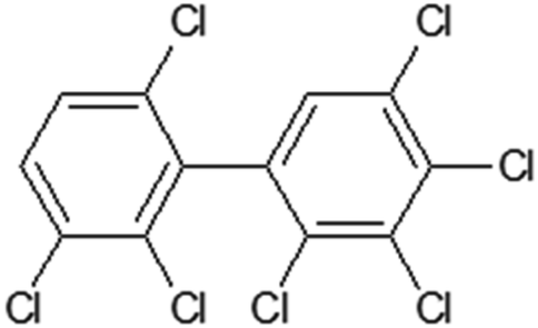
Table 1 contains the general scheme of the DCW(1,15) calculation for 2,2′,3,3′,4,5,6′-heptachlorobiphenyl (Fig. 1). Some parameters are shared in CORAL, while at the end of Table 1, there are the local symmetry fragments (LSF). In some cases, the symbol ‘x’ is equal to the symbol ‘z’. These SMILES attributes are associated with correlation weights (CW), as in eqn (1). The CW may have a positive or negative sign, depending on their role in modeling the Henry constant. The value of the CW suggests the importance of each SMILES attribute. The statistical defect of SMILES attributes indicates the measure of their prevalence: a low value (0.001 or less) indicates that the attribute is not rare.
Table 1 The scheme of DCW(1,15) calculation for 2,2′,3,3′,4,5,6′-heptachlorobiphenyl represented by SMILES = Clc1c(c(cc(c1Cl)c1c(ccc(c1Cl)Cl)Cl)Cl)Cla
| SMILES attribute |
Correlation weight |
Statistical defect |
|
The local symmetry fragments (LSF) are defined as follows: [xyx8] = c1c;c(c;(c(;c(c;c(c;c1c;c(c;c(c: [xyyx1] = (cc(: [xyzyx2] = c(c(c;(ccc(.
|
|
S
k
|
| Cl……… |
1.3661 |
0.00418 |
| c……… |
−0.0459 |
0.00251 |
| 1……… |
−0.6212 |
0.00238 |
| c……… |
−0.0459 |
0.00251 |
| (……… |
−0.6125 |
0.00021 |
| c……… |
−0.0459 |
0.00251 |
| (……… |
−0.6125 |
0.00021 |
| c……… |
−0.0459 |
0.00251 |
| c……… |
−0.0459 |
0.00251 |
| (……… |
−0.6125 |
0.00021 |
| c……… |
−0.0459 |
0.00251 |
| 1……… |
−0.6212 |
0.00238 |
| Cl……… |
1.3661 |
0.00418 |
| (……… |
−0.6125 |
0.00021 |
| c……… |
−0.0459 |
0.00251 |
| 1……… |
−0.6212 |
0.00238 |
| c……… |
−0.0459 |
0.00251 |
| (……… |
−0.6125 |
0.00021 |
| c……… |
−0.0459 |
0.00251 |
| c……… |
−0.0459 |
0.00251 |
| c……… |
−0.0459 |
0.00251 |
| (……… |
−0.6125 |
0.00021 |
| c……… |
−0.0459 |
0.00251 |
| 1……… |
−0.6212 |
0.00238 |
| Cl……… |
1.3661 |
0.00418 |
| (……… |
−0.6125 |
0.00021 |
| Cl……… |
1.3661 |
0.00418 |
| (……… |
−0.6125 |
0.00021 |
| Cl……… |
1.3661 |
0.00418 |
| (……… |
−0.6125 |
0.00021 |
| Cl……… |
1.3661 |
0.00418 |
| (……… |
−0.6125 |
0.00021 |
| Cl……… |
1.3661 |
0.00418 |
![[thin space (1/6-em)]](https://www.rsc.org/images/entities/char_2009.gif) |
|
SS
k
|
| c⋯Cl…… |
1.7521 |
0.00962 |
| c…1…… |
−0.0002 |
0.00251 |
| c…1…… |
−0.0002 |
0.00251 |
| c…(…… |
−0.3031 |
0.00316 |
| c…(…… |
−0.3031 |
0.00316 |
| c…(…… |
−0.3031 |
0.00316 |
| c…(…… |
−0.3031 |
0.00316 |
| c…c…… |
0.1630 |
0.00264 |
| c…(…… |
−0.3031 |
0.00316 |
| c…(…… |
−0.3031 |
0.00316 |
| c…1…… |
−0.0002 |
0.00251 |
| Cl…1…… |
−0.8813 |
0.00908 |
| Cl…(…… |
−0.0033 |
0.00465 |
| c…(…… |
−0.3031 |
0.00316 |
| c…1…… |
−0.0002 |
0.00251 |
| c…1…… |
−0.0002 |
0.00251 |
| c…(…… |
−0.3031 |
0.00316 |
| c…(…… |
−0.3031 |
0.00316 |
| c…c…… |
0.1630 |
0.00264 |
| c…c…… |
0.1630 |
0.00264 |
| c…(…… |
−0.3031 |
0.00316 |
| c…(…… |
−0.3031 |
0.00316 |
| c…1…… |
−0.0002 |
0.00251 |
| Cl…1…… |
−0.8813 |
0.00908 |
| Cl…(…… |
−0.0033 |
0.00465 |
| Cl…(…… |
−0.0033 |
0.00465 |
| Cl…(…… |
−0.0033 |
0.00465 |
| Cl…(…… |
−0.0033 |
0.00465 |
| Cl…(…… |
−0.0033 |
0.00465 |
| Cl…(…… |
−0.0033 |
0.00465 |
| Cl…(…… |
−0.0033 |
0.00465 |
| Cl…(…… |
−0.0033 |
0.00465 |
|
|
Local symmetry fragments (LSF)
|
| [xyx8]…… |
−0.3984 |
0.00855 |
| [xyyx1]… |
0.3706 |
0.00120 |
| [xyzyx2]… |
2.2237 |
0.00445 |
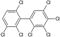 |
| | Fig. 1 The structure of 2,2′,3,3′,4,5,6′-heptachlorobiphenyl. | |
2.3 The Monte Carlo optimization
Eqn (2) needs the numerical data on the CW. The Monte Carlo optimization serves to calculate them. Here two target functions for the Monte Carlo optimization are examined:| | | TF0 = rAT + rPT − |rAT − rPT| × 0.1 | (2) |
| | | TF1 = TF0 + IICC × WIIC + CIIC × WCII | (3) |
r
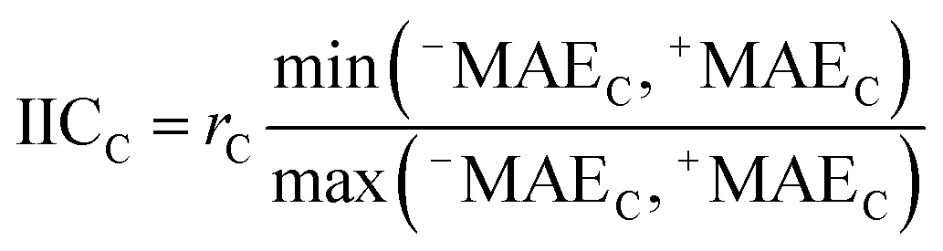
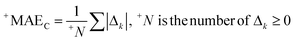
AT and rPT are correlation coefficients between the observed and predicted endpoints for the active and passive training sets, respectively. IICC is the index of ideality of correlation.13,16 IICC is calculated with data on the calibration set as follows:
| |  | (4) |
| |  | (5) |
| |  | (6) |
| |  | (7) |
| |  | (8) |
| | | Δk = observedk − calculatedk | (9) |
The observed and calculated are corresponding values of the endpoint.
The correlation intensity index (CII), similarly to the IIC, was developed as a tool to improve the quality of the Monte Carlo optimization aimed to build up QSPR/QSAR models.
The CII is calculated as follows:17
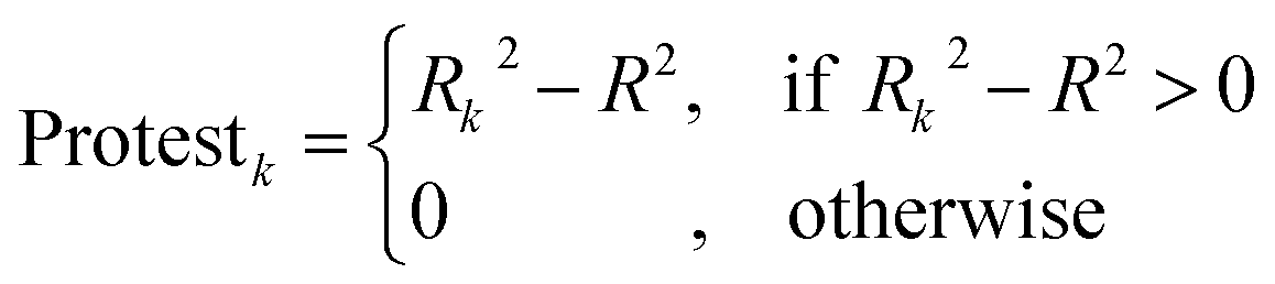
| |  | (11) |
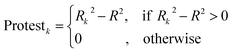
R
2 is the correlation coefficient for a set containing n substances. Rk2 is the correlation coefficient for n − 1 substances of a set after removing of k-th substance. Thus, if the (Rk2 − R2) is larger than zero, the k-th substance counteracts the correlation between the experimental and predicted values of the set. A small sum of “protests” means a better correlation.
The numerical values of weights W_IIC and W_CII for eqn (3) were selected from the preliminary computational experiments (Table 2). One can see that 0.3 is the best value for these weights. It should be noted that using IIC and CII improves the statistical quality of models for external validation sets to the detriment of training sets. Nevertheless, this effect is more of an advantage than a disadvantage.13,16,18,19
Table 2 The determination coefficients (R2) on the calibration set were observed for different combinations of weights for IIC and CII
|
|
WIIC = 0.2 |
WIIC = 0.3 |
WIIC = 0.4 |
| WCII = 0.2 |
0.7256 |
0.7214 |
0.7234 |
| WCII = 0.3 |
0.7096 |
0.7598 |
0.7311 |
| WCII = 0.4 |
0.7020 |
0.7222 |
0.7143 |
3. Results and discussion
3.1 Selection of the CORAL-method
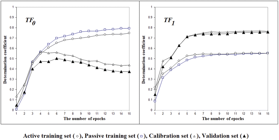
Fig. 2 shows the histories of the Monte Carlo optimization with target functions TF0 (eqn (2), without the IIC and CII) and with TF1 (eqn (3), using the IIC and CII). In the case of target function TF0 the determination coefficients for the calibration and validation sets are lower than with the target function TF1. Thus, one can see (Fig. 2) that the preferable way to generate QSPR models is the Monte Carlo optimization with target function TF1 because this offers better results when predicting new substances, which is the case of the results with the validation set. Furthermore, the spread between the values of the training sets and the others is smaller, which is also preferable, indicating more stable results.
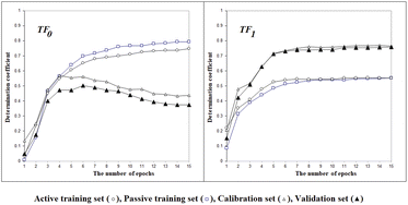 |
| | Fig. 2 The general scheme of the epoch sequence of Monte Carlo optimization for the target functions TF0 and TF1. | |
The next point is to evaluate whether taking into account the LSF represented by three- (‘xyx’), four- (‘xyyx’), and five (‘xyzyx’) symbol configurations. Fig. 3 indicates that the LSF give significant improvement for the calibration set. This feature is a specific characteristic allowed by the use of the representation of the chemical structure as implicit in the CORAL model. Indeed, the symmetry is applied not to the whole molecule but to the individual SMILES attribute: in this case, to the sequence of characters in the SMILES. Thus, this feature represents a situation of local symmetry within the larger structure of the molecule. These particular molecular components help predict the physicochemical property under study better. The sign associated with these SMILES attributes is positive. If at least part of the molecule is symmetrical, it increases the possibility of forming intramolecular bonds between different molecules in the liquid phase, thus reducing Henry's constant value.
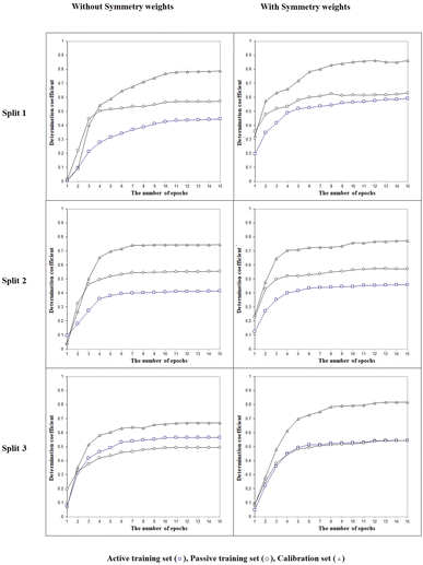 |
| | Fig. 3 The general scheme of the epoch sequence of the Monte Carlo optimization for three splits with and without considering the local symmetry fragments into account. | |
3.2 QSPR-models for Henry's law constants
As indicated above, we developed QSPR models with different settings to predict Henry's law constants. The results were best with TF1 and LSF. Table 3 lists the statistical characteristics of these models for three splits of the set of compounds.
Table 3 Statistical characteristics of Henry's law constants models for splits #1, #2, and #3a
| Split |
Set* |
n
|
R
2
|
CCC |
IIC |
CII |
Q
2
|
|
A = active training set; P = passive training set; C = calibration set; V = validation set; n = the number of compounds in a set; R2 = determination coefficient; CCC = concordance correlation coefficient; IIC = index of ideality of correlation; CII = correlation intensity index; Q2 = leave-one-out cross-validated R2; QF12, QF22, and QF32 = the statistical criteria suggested in the literature;20 〈Rm2〉 = the average Rm2 metric.21
|
| 1 |
A
|
132 |
0.5281 |
0.6912 |
0.6244 |
0.7675 |
0.5051 |
|
|
P
|
133 |
0.6175 |
0.7179 |
0.6621 |
0.7900 |
0.6058 |
|
|
C
|
127 |
0.8375 |
0.9150 |
0.9152 |
0.9030 |
0.8307 |
|
|
V
|
135 |
0.7388 |
0.8582 |
|
|
|
|
|
|
Q
F1
2
|
Q
F2
2
|
Q
F3
2
|
〈Rm2〉 |
RMSE |
MAE |
|
|
A
|
|
|
|
|
1.59 |
1.34 |
|
|
P
|
|
|
|
|
1.66 |
1.38 |
|
|
C
|
0.8369 |
0.8327 |
0.9444 |
0.7697 |
0.580 |
0.434 |
|
|
V
|
|
|
|
|
0.641 |
0.434 |
|
|
|
n
|
R
2
|
CCC |
IIC |
CII |
Q
2
|
| 2 |
A
|
131 |
0.5075 |
0.6733 |
0.6600 |
0.7484 |
0.4922 |
|
|
P
|
133 |
0.6233 |
0.7591 |
0.7362 |
0.8083 |
0.6084 |
|
|
C
|
130 |
0.8332 |
0.9064 |
0.9128 |
0.9069 |
0.8240 |
|
|
V
|
133 |
0.7739 |
0.8862 |
|
|
|
|
|
|
Q
F1
2
|
Q
F2
2
|
Q
F3
2
|
〈Rm2〉 |
RMSE |
MAE |
|
|
A
|
|
|
|
|
1.60 |
1.33 |
|
|
P
|
|
|
|
|
1.65 |
1.40 |
|
|
C
|
0.8309 |
0.8304 |
0.9473 |
0.7604 |
0.555 |
0.444 |
|
|
V
|
|
|
|
|
0.649 |
0.500 |
|
|
|
n
|
R
2
|
CCC |
IIC |
CII |
Q
2
|
| 3 |
A
|
132 |
0.5939 |
0.7452 |
0.7477 |
0.7704 |
0.5771 |
|
|
P
|
131 |
0.5423 |
0.7174 |
0.6098 |
0.7879 |
0.5241 |
|
|
C
|
131 |
0.7861 |
0.8823 |
0.8856 |
0.8740 |
0.7793 |
|
|
V
|
133 |
0.7540 |
0.8551 |
|
|
|
|
|
|
Q
F1
2
|
Q
F2
2
|
Q
F3
2
|
〈Rm2〉 |
RMSE |
MAE |
|
|
A
|
|
|
|
|
1.56 |
1.28 |
|
|
P
|
|
|
|
|
1.72 |
1.40 |
|
|
C
|
0.7794 |
0.7601 |
0.9306 |
0.7004 |
0.646 |
0.518 |
|
|
V
|
|
|
|
|
0.696 |
0.532 |
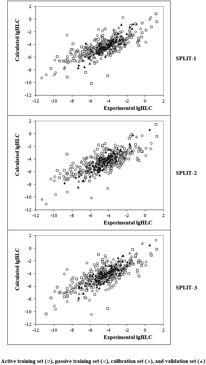
Fig. 4 contains the graphical representation of models observed for the cases of splits 1, 2, and 3. The best model observed for the split 2 (determination coefficient on the calibration set is 0.8332). The model is the following:
| | | lgHLC = −4.653 (±0.012) + 0.3277 (±0.0025) × DCW(1,15) | (12) |
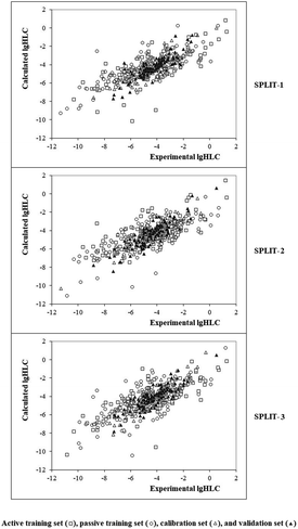 |
| | Fig. 4 Graphical representation of models obtained using the Monte Carlo optimization based on target function TF1. | |
The ESI† section contains the list of correlation weights of the model (Table S3†).
For 2,2′,3,3′,4,5,6′-heptachlorobiphenyl (Table 1) the model, is the following:
| lgHLC = −4.653 + 0.3277 × (−0.2894) = −4.7484 |
The ESI† section contains the technical details on models obtained for three random splits studied here.
3.3 Applicability domain
The largest number of suspected outliers according to the statistical defect14 (over three different splits) is seven. Thus, most compounds examined here were not outliers.
There are some compounds which are outliers for all three models. The molecular features that unite these emissions are:
• The presence of a triple bond;
• The presence of chlorine;
• The presence of a large number of rings.
The diapason of lgHLC for the examined models ranges in the interval (−12.99, 1.30).
3.4 Mechanistic interpretation
Sulfur, the presence of three cycles, and double bonds of carbon and oxygen turned out to be promoters of the decrease in constants. All these chemical fragments are associated with the molecule's polarity, which reduces its volatility. The promoters of increase turned out to be the branching of the atomic framework, aromaticity, as well as the presence of ‘xyx’ and ‘xyzyx’ fragments local symmetry. These components refer to steric factors related to more structures that are rigid. Thus, these compounds can establish intermolecular binding in the liquid phase with greater difficulty, which explains that they are associated with an increase in Henry's law constant. Regarding the symmetry fragments, we observe that they are present in branched aromatic or polycyclic molecules, as implicit in their structure, indicated in Section 2.2: c1c;(c(;c1c;c(c(c;(ccc(. Thus, the interpretation of the role of SMILES fragments for the statistical quality of the model is suggested.
3.5 Comparison with models suggested in the literature
Table 4 compares the statistical quality of models for Henry's law constants suggested in the literature. The determination coefficient and RMSE for the calibration and validation set suggested by Duchowicz et al.2 are n = 176, D = 0.85, RMSE = 0.70 (calibration set) and n = 177, D = 0.81, RMSE = 0.71 (validation set). These values are important since the present study refers to the same dataset. The models from the literature for Henry's law constants,2 obtained using and analysing a large pool of physicochemical and 3D descriptors, gave results with predictive potential similar to those we obtained here. However, the data processing in our case is much simpler since it does not require the calculation of chemical descriptors and successive algorithm implementation.
Table 4 Comparison of the statistical characteristics of different models for Henry's law constants
|
N
train
|
R
train
2
|
RMSEtrain |
N
val
|
R
val
2
|
RMSEval |
Software |
| 700 |
0.88 |
1.03 |
— |
— |
— |
HENRYWIN1 |
| 588 |
0.90 |
0.92 |
— |
— |
— |
HENRYWIN1 |
| 310 |
0.96 |
0.67 |
— |
— |
— |
HENRYWIN10 |
| 128 |
0.94 |
— |
— |
— |
— |
ANN9 |
| 1339 |
0.84 |
1.25 |
— |
— |
— |
US EPA22 |
| 110 |
0.69 |
2.0 |
— |
— |
— |
US EPA7 |
| 29 |
0.93 |
1.12 |
19 |
0.65 |
— |
GA MLR6 |
| 177 |
0.87 |
0.85 |
177 |
0.85 |
0.71 |
Replacement method2 |
| 392 |
0.60 |
1.37 |
135 |
0.74 |
0.64 |
This work |
The group of models in Table 4 is characterized by different statistical qualities. Our results are paradoxical since the statistical quality of the models for the calibration and validation sets is higher than for the training (active and passive) sets (Table 3). Similar situations were observed in analogous computer experiments designed to develop models of other endpoints.16,18,19 It seems reasonable to assess the results of this work as quite promising.
4. Conclusions
The fragments of local symmetry introduced here can improve the quality of the optimal (flexible) descriptors calculated with SMILES. The predictive potential of models for Henry's law constants when applying the correlation weights for local symmetry is significantly better than for models built up without taking these SMILES attributes into account. The suggested models can quickly assess large groups of potential atmospheric contaminants, as is needed to address their impact on climate change and their suitability as safe substances from an ecological point of view.
Data availability
The data used in this work and the models developed are freely available in the ESI† section.
Author contributions
Conceptualization, A. A. T., A. P. T., A. R., and E. B.; methodology, A. A. T., A. P. T., A. R., and E. B.; software, A. A. T.; validation, A. A. T., A. P. T., A. R., and E. B.; formal analysis, A. P. T.; data curation, A. P. T., A. A. T.; writing—original draft preparation, A. A. T., A. P. T.; writing—review and editing, A. A. T., A. P. T., A. R., and E. B.; supervision, E. B. All authors have read and agreed to the published version of the manuscript.
Conflicts of interest
The authors declare that they have no known competing financial interests or personal relationships that could have influenced the work reported in this paper.
Acknowledgements
This work was supported by CONCERT REACH, grant agreement LIFE17 GIE/IT/000461.
References
- J. C. Dearden and G. Schüürmann, Quantitative structure-property relationships for predicting henry's law constant from molecular structure, Environ. Toxicol. Chem., 2003, 22, 1755–1770, DOI:10.1897/01-605.
- P. R. Duchowicz, J. F. Aranda, D. E. Bacelo and S. E. Fioressi, QSPR study of the Henry's law constant for heterogeneous compounds, Chem. Eng. Res. Des., 2020, 154, 115–121, DOI:10.1016/j.cherd.2019.12.009.
- P. R. Duchowicz, J. C. M. Garro and E. A. Castro, QSPR study of the Henry's Law constant for hydrocarbons, Chemom. Intell. Lab. Syst., 2008, 91(2), 133–140, DOI:10.1016/j.chemolab.2007.10.005.
- F. Gharagheizi, P. Ilani-Kashkouli, S. A. Mirkhani, N. Farahani and A. H. Mohammadi, QSPR molecular approach for estimating Henry's law constants of pure compounds in water at ambient conditions, Ind. Eng. Chem. Res., 2012, 51(12), 4764–4767, DOI:10.1021/ie202646u.
- T. Puzyn and J. Falandysz, QSPR modeling of partition coefficients and Henry's law constants for 75 chloronaphthalene congeners by means of six chemometric approaches - A comparative study, J. Phys. Chem. Ref. Data, 2007, 36(1), 203–214, DOI:10.1063/1.2432888.
- A. Bouakkadia, Y. Driouche, N. Kertiou and D. Messadi, Modeling of the henry constant of a series of pesticides: Quantitative structure-property relationship approach, Int. J. Saf. Secur. Eng., 2020, 10(3), 389–396, DOI:10.18280/ijsse.100311.
- C. I. Nicolas, K. Mansouri, K. A. Phillips, C. M. Grulke, A. M. Richard, A. J. Williams, J. Rabinowitz, K. K. Isaacs, A. Yau and J. F. Wambaugh, Rapid experimental measurements of physicochemical properties to inform models and testing, Sci. Total Environ., 2018, 636, 901–909, DOI:10.1016/j.scitotenv.2018.04.266.
- J. Long, Q. Youli and L. Yu, Effect analysis of quantum chemical descriptors and substituent characteristics on Henry's law constants of polybrominated diphenyl ethers at different temperatures, Ecotoxicol. Environ. Saf., 2017, 145, 176–183, DOI:10.1016/j.ecoenv.2017.07.024.
- D. R. O'Loughlin and N. J. English, Prediction of Henry's Law Constants via group-specific quantitative structure property relationships, Chemosphere, 2015, 127, 1–9, DOI:10.1016/j.chemosphere.2014.11.065.
- W. M. Meylan and P. H. Howard, Estimating octanol-air partition coefficients with octanol-water partition coefficients and Henry's law constants, Chemosphere, 2005, 61(5), 640–644, DOI:10.1016/j.chemosphere.2005.03.029.
- D. Weininger, SMILES, a Chemical Language and Information System: 1: Introduction to Methodology and Encoding Rules, J. Chem. Inf. Comput. Sci., 1988, 28(1), 31–36, DOI:10.1021/ci00057a005.
- A. A. Toropov, A. P. Toropova, T. Puzyn, E. Benfenati, G. Gini, D. Leszczynska and J. Leszczynski, QSAR as a random event: Modeling of nanoparticles uptake in PaCa2 cancer cells, Chemosphere, 2013, 92(1), 31–37, DOI:10.1016/j.chemosphere.2013.03.012.
- A. A. Toropov, R. Carbó-Dorca and A. P. Toropova, Index of Ideality of Correlation: new possibilities to validate QSAR: a case study, Struct. Chem., 2018, 29(1), 33–38, DOI:10.1007/s11224-017-0997-9.
- A. A. Toropov, A. P. Toropova, M. Marzo, J. L. Dorne, N. Georgiadis and E. Benfenati, QSAR models for predicting acute toxicity of pesticides in rainbow trout using the CORAL software and EFSA's OpenFoodTox database, Environ. Toxicol. Pharmacol., 2017, 53, 158–163, DOI:10.1016/j.etap.2017.05.011.
- A. P. Toropova, A. A. Toropov, S. E. Martyanov, E. Benfenati, G. Gini, D. Leszczynska and J. Leszczynski, CORAL: QSAR modeling of toxicity of organic chemicals towards Daphnia magna, Chemom. Intell. Lab. Syst., 2012, 110(1), 177–181, DOI:10.1016/j.chemolab.2011.10.005.
- A. P. Toropova and A. A. Toropov, The index of ideality of correlation: A criterion of predictability of QSAR models for skin permeability?, Sci. Total Environ., 2017, 586, 466–472, DOI:10.1016/j.scitotenv.2017.01.198.
- A. A. Toropov and A. P. Toropova, QSAR as a random event: criteria of predictive potential for a chance model, Struct. Chem., 2019, 30(5), 1677–1683, DOI:10.1007/s11224-019-01361-6.
- A. P. Toropova, A. A. Toropov, A. Roncaglioni and E. Benfenati, The index of ideality of correlation improves the predictive potential of models of the antioxidant activity of tripeptides from frog skin (Litoria rubella), Comput. Biol. Med., 2021, 133, 104370, DOI:10.1016/j.compbiomed.2021.104370.
- A. P. Toropova, A. A. Toropov, E. L. Viganò, E. Colombo, A. Roncaglioni and E. Benfenati, Carcinogenicity prediction using the index of ideality of correlation, SAR QSAR Environ. Res., 2022, 33(6), 419–428, DOI:10.1080/1062936X.2022.2076736.
- V. Consonni, D. Ballabio and R. Todeschini, Comments on the definition of the Q2 parameter for QSAR validation, J. Chem. Inf. Model., 2009, 49(7), 1669–1678, DOI:10.1021/ci900115y.
- P. K. Ojha, I. Mitra, R. N. Das and K. Roy, Further exploring rm2 metrics for validation of QSPR models, Chemometr. Intell. Lab. Syst., 2011, 107(1), 194–205, DOI:10.1016/j.chemolab.2011.03.01.
-
US EPA, Estimation Programs Interface Suite TM for Microsoft® Windows, United States Environmental Protection Agency, Washington, DC, USA, 411 edn, 2016, https://www.epa.gov/tsca-screening-tools/epi-suitetm-estimation-program-interface Search PubMed.
|
| This journal is © The Royal Society of Chemistry 2023 |
Click here to see how this site uses Cookies. View our privacy policy here. 
 Open Access Article
 This Open Access Article is licensed under a Creative Commons Attribution-Non Commercial 3.0 Unported Licence
 ,
Alla P.
Toropova
,
Alla P.
Toropova