
 Open Access Article
 This Open Access Article is licensed under a
 Creative Commons Attribution 3.0 Unported Licence
Conceptualizing turbidity for aquatic ecosystems in the context of sustainable development goals†
D.
Sahoo
 *a and
A.
Anandhi
b
*a and
A.
Anandhi
b
aClemson University, 509 Westinghouse Rd, Pendleton, SC 29670, USA. E-mail: dsahoo@clemson.edu
bFlorida A&M University, USA
First published on 4th August 2023
Abstract
Understanding water quality is important to assess water security including the health of the society and the nation. Turbidity is one of the critical parameters to assess the quality of water in aquatic ecosystems. It can affect various eco-hydrological processes, directly or indirectly. The objectives of the current study were to (a) conceptualize turbidity based on the available literature through system-level thinking to synthesize the eco-hydrological processes, (b) understand the relationship between turbidity, processes and Sustainable Development Goals (SDGs), and (c) apply the conceptual model to turbidity data obtained from the Reedy River Watershed in South Carolina, USA. The application would improve the understanding of the stakeholders in making informed decisions to manage turbidity. The developed conceptual model identified drivers of turbidity in SDGs 2, 7, 11, 13, 14 and 15 and identified impacts of turbidity in SDGs 2, 3, 5, 6, 7, 8, 10, 13, 14 and 15. This model was applied to hysteresis and cumulative frequency analysis to identify several key watershed processes that impacted turbidity. The sites that were analyzed in general indicated negative hysteresis. On one occasion, one of the sites marked positive hysteresis. Generally, in urban areas, with a higher percentage of imperviousness, there is an exhaustion of sediment, which could be one explanation for negative hysteresis. Cumulative frequency plots indicated that larger storms caused the majority of sediment and exceeded the limit 10–15% of the time. While the steps of conceptualizing turbidity can be universally applied to all locations, the specific goals and targets identified in this analysis may vary depending on the chosen location. The processes adopted in this framework help in understanding various environmental implications of turbidity. These types of analysis will be of importance for water resources managers to obtain a comprehensive overview of sustainable watershed management, which in turn will contribute to achieving the UN SDGs.
Environmental significanceWith increasing land use and climate change, water quantity and quality issues will continue to challenge researchers, engineers, practitioners, and policymakers in the foreseeable future. An understanding of these issues concerning UN Sustainable Development Goals (SDGs) would help resource managers to address the environmental challenges holistically. In the current work, the authors used turbidity, an indicator of water quality to conceptualize and understand its relationship with various SDGs. The approach examined on an available turbidity dataset from a watershed located in the upstate region of South Carolina (SC), USA. A similar framework can be developed and applied to address various water and environmental issues. |
Introduction
Despite global efforts to achieve water security, in 2011, nearly 0.9 billion did not have sufficient access to safe water,1 and in 2016 nearly 2.1 billion people lack access to safely managed drinking water.2 The scarcities of water resources pose numerous challenges including social and political insecurities, geopolitical conflicts, irremediable environmental damages and even loss of life.3 For instance, a breakdown of 4.3 million deaths per year is found to be associated with air pollution when ∼2.9 billion people are using some form of biomass for cooking and heating, and contaminated water when 1.8 billion people rely on faecal contaminated drinking water sources.4 Several water quality parameters such as dissolved oxygen (DO), pH, specific conductivity, turbidity etc. affect the health of freshwater water systems and are influenced by anthropogenic and natural conditions. Unlike water temperature and pH, turbidity is not an inherent water property.5 It is one of the key parameters that have a significant impact on the water quality of the lotic and lentic systems. Elevated turbidity could significantly deteriorate the aesthetic quality of the streams, rivers, and lakes, impacting the recreational value of the resources. Furthermore, high turbidity values could increase the drinking water treatment cost, impact irrigation, and damage aquatic life, and other societal and ecological uses. Due to the varied impacts of turbidity on aquatic systems, drinking water security and the end-users, different states have freshwater turbidity standards for streams and lakes.6 Given its significance to ecological and hydrological ecosystems, turbidity has gained attention in recent times.Turbidity is a measure of the extent to which water loses its transparency due to the presence of suspended particulates such as sediment, inorganic suspended materials, organic matter, soluble coloured organic compounds, phytoplankton, algae, and other microscopic organisms. The presence of suspended matter in the water column absorbs or scatters the downwelling light that causes turbidity in the water column.7 Although several factors influence turbidity, often suspended sediment is the key factor contributing to turbidity in the aquatic ecosystem. Suspended sediment is generally well correlated with turbidity. Therefore, the measurement of turbidity is relatively inexpensive and could be used as an indicator of sediment concentration. Different instruments use different methods to measure turbidity. The clarity is used to represent turbidity and is measured using in situ disk (Secchi disk, black disk) measurement and light transmissometer techniques.8 Turbidity is typically measured by light sensors. The sensor sends light at a certain wavelength and measures the amount of scattered light. Although the instruments use light primarily, the type of light, number of sensors, number of beams, and measurement of the light could also influence turbidity.8 Because different instruments use different techniques, the same sample would read a different value when measured by different instruments at the same time. While in situ instruments provide accurate turbidity measurements at a given location, they do not provide the spatial distribution of turbidity. More recently, remote sensing technologies have been very beneficial in measuring turbidity from space to capture a larger spatial scale. Turbidity can be analyzed in the lab in addition to remote sensing and in situ sensors. Computer models (e.g., Soil and Water Assessment Tool (SWAT), Loading Simulation Program in C++ (LSPC)) can model sediment transport and turbidity can be used as a surrogate to capture sediment loading. The common units of turbidity are the Nephelometric Turbidity Unit (NTU) and Formazin Turbidity Unit (FTU) used in various in situ instruments. There are other units such as Nephelometric Ratiometric Turbidity Units (NTRUs), Formazin Nephelometric Unit (FNU), Formazin Ratiometric Turbidity Unit (FNRU), Formazin Backscatter Unit (FBU), Nephelometric Turbidity Multibeam Unit (NTMU) and Formazin Nephelometric Multibeam Unit (FNMU).
When turbidity in a waterbody crosses the regulated limit, the waterbody is considered impaired for turbidity. Programs are developed to address the concerns and limit the pollutant's concentration in the waterbody within the permissible boundary that maintains a healthy ecosystem. In South Carolina, a 50 NTU standard is required for streams and rivers and a 25 NTU standard is required for lakes and reservoirs. The USEPA states that turbidity should not be more than 1 NTU at any given time and it should be less than or equal to 0.3 NTUs in at least 95 percent of the samples in any given month for conventional or direct filtration. For systems that use filtration other than conventional or direct filtration should follow the state standard and must include turbidity not exceeding 5 NTU at any given time.9
Turbidity is, directly and indirectly, connected to as well as essential in achieving most of the 17 Sustainable Development Goals (SDGs). Understanding water, including it's quality is crucial for sustainable development and supporting life on Earth. Turbidity shapes several ecological and hydrological processes directly and indirectly. Hence, they touch most, if not all, of the SDGs, specifically SDG 6 (water).2 Water resources are under significant stress and are experiencing high demand which is further exacerbated by increasing pressure from expanding population, globalization, rapid economic growth, unsustainable urbanization, increased demand for land,10 climate change, land use and lifestyle changes, and more recently due to the COVID-19 pandemic. In recent times, turbidity has been used to assess the direct or indirect impacts of COVID-19. Studies11,12 indicated that lockdown during COVID-19 improved the riverine water quality. Although turbidity and SDGs are studied independently, their combined relationship has not been well documented. This study attempts to address this need by conceptualizing the relationship.
Conceptualizations are carried out using conceptual models/frameworks and are regarded as organizational diagrams.13–15 They are useful in collating, visualizing, understanding, and explaining the problems/situations and how they might be solved by bringing together and summarizing information in a standard, logical, and hierarchical way.16–18 They guide research to deliver the necessary insights into key system aspects and increase its understanding.19,20 Although conceptualizations are probably the most important activity to be carried out in a simulation study, they are often ignored because it is the most difficult and least understood part of a simulation study.21,22
While all the previous turbidity studies have focused on the causes and impacts of turbidity in aquatic ecosystems, the current study attempts to conceptualize turbidity of aquatic ecosystems in the context of SDGs. The novelty of this study is to conceptualize them using systems thinking.
The objectives of the study were-
(1) Utilize the systems thinking approach to conceptualize turbidity in terms of how it, directly and indirectly, interacts with some of the ecological and hydrological processes.
(2) Conceptualize the relationship between turbidity and SDGs employing the identified processes in objective 1 and develop a conceptual model.
(3) Apply the conceptual model to a case study: Reedy River Watershed in South Carolina to improve understanding of turbidity in the context of SDGs and its understanding to support stakeholders in making informed decisions.
Materials and methods
In step 1, to conceptualize turbidity, an exhaustive literature search was conducted on turbidity on Google scholar. Keywords related to turbidity (e.g., turbidity, ecological processes, hydrological processes) were used to obtain relevant articles. The articles that contain information on the important factors (e.g., hydrological, ecological) were identified. Since turbidity can directly or indirectly affect various hydrological or ecological processes, each article was further classified accordingly. The symbols that were used for the causes and the effects of the processes while categorizing the articles were-hydrological processes (H), ecological processes (E), general processes (G, i.e., factors other than hydrological and ecological processes), directly (D) and indirectly (I). Once the articles were classified based on either H, E, G, D, or I, the articles were further rearranged again in a tabular format for a better conceptualization of turbidity, likely allowing for a clearer understanding of the information contained in the articles.In step 2, the conceptualization of turbidity was achieved by system thinking where the relationship was established between the components forming the purposeful whole. SDGs drivers of turbidity (e.g., climate change), and impacts of turbidity were the components.23 Further, the targets of the identified SDGs were conceptualized into “high”, “medium”, “low” and “no relevance” to turbidity. Targets classified as having “high” relevance are highly likely to happen in the study region and directly impact turbidity through interventions (e.g., technological, social, administrative, or economic). Targets classified as having “moderate” relevance are moderately likely to happen in the study region and affect turbidity through interventions (e.g., technological, social, administrative, or economic). Targets are classified as having “low” relevance if they are unlikely to happen very often in the study region or only indirectly impact turbidity through interventions (e.g., technological, social, administrative, or economic). The approach to assessing the relevance of the SDGs is described in the “Methods” section.
In step 3, hysteresis (e.g., flow and turbidity) was used as an indicator of various processes associated with turbidity and was further linked with various classes and SDGs. Classes are based on peak flow and peak turbidity.24
In step 4, as an example, turbidity hysteresis24,25 was estimated, analysed, and explained in the context of various process understandings (e.g., drivers, impacts) and SDGs utilizing data collected in the Reedy River Watershed in South Carolina. In addition to turbidity hysteresis, turbidity exceedance plots were created to understand the regulatory violations and flow-based turbidity analysis was conducted to assess the flow regime, storm events and associated turbidity. Details regarding the sites are discussed in the “Study Area Description” of this article.
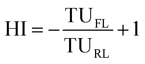
Hysteresis analysis was conducted by computing Hysteresis index (HI) values,24 which can be used to determine if turbidity is influenced by a local source or a non-local source and could help understand sediment contributions from developed and undeveloped watersheds. The below set of equations is used to estimate HI.
For TURL > TUFL,
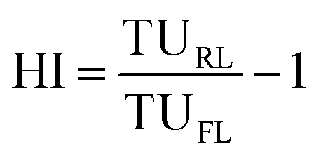
For TUFL > TURL,
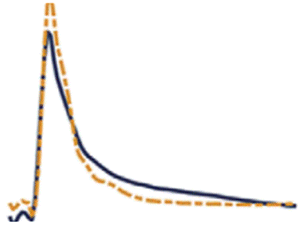
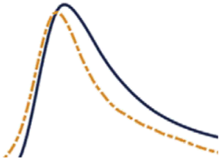
A hysteresis index value was calculated at flow rates equal to 25 percent of the maximum storm event flow, 50 percent of the maximum storm event flow, and 75 percent of the maximum storm event flow (Fig. 1). Using three intermediate values for each storm event gives an index value that better represents the overall hysteresis of the storm event, rather than using only a single point on the hydrograph. These three index values were averaged to give a hysteresis index value for each storm event at each Reedy River monitoring station. The hysteresis index can be either positive or negative depending on the shape of the hysteresis plot.
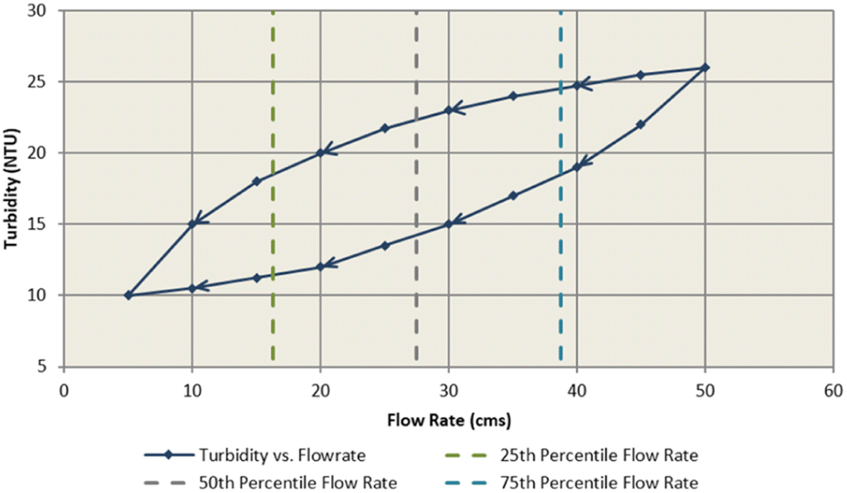 | ||
| Fig. 1 Example of a turbidity hysteresis. Each point represents a water quality reading. The readings for the duration of an event are plotted, with arrows connecting subsequent readings in chronological order. The flow rates equal to 25 percent of the maximum storm event flow, 50 percent of the maximum storm event flow, and 75 percent of the maximum storm event flow are identified to estimate the HI. Additional information is included in the ESI Materials.† | ||
A cumulative frequency analysis was conducted on the daily average turbidity datasets at each station for the period of analysis. The results help understand the exceedances of turbidity in freshwater streams and rivers based on the regulatory standard of 50 NTU in South Carolina. In this analysis, the daily average turbidity value is plotted against the fraction of time that the parameter was observed to be at or below that value. Cumulative frequency plots provide a detailed view of the shape of a parameter's distribution and can help understand the impact of the watershed processes. They can be useful in demonstrating unusual patterns in turbidity of a stream that occur at only certain ranges of the distribution.
To better understand the influence of storm events on turbidity, the turbidity dataset was parsed according to the corresponding flow rate. The turbidity data were divided into subsets corresponding to each of the flow duration exceedance percentiles. Box and whisker plots were then constructed for each of these data subsets, and these were plotted in order from the highest flow range to the lowest flow range. Analyzing the data in this way allows for general observations to be drawn regarding the impact of storm events on turbidity in the river system.
Study area description and dataset of the case study
Greenville County, South Carolina, a Phase-1 Municipal Separate Storm Sewer System (MS4), has been collecting various high frequency (e.g., 15 minutes) continuous real-time water quality information (e.g., turbidity, dissolved oxygen, pH, conductivity, temperature, stage) at strategic locations in the Reedy River as a part of the NPDES permit since 2008. The two sites that were used in the current analysis, are part of the monitoring efforts. The two sites are Hudson, upstream of the City of Greenville, SC. and Parkins, downstream of the City of Greenville, SC (Fig. 2). Data from the two permit years, July 2013–June 2014, and July 2014–June 2015 were used for the current investigation due to the availability and accessibility of the data. While the dataset is from one location and collected for two years, some of the analysis and results derived concerning SDGs can still provide meaningful insights into the processes affecting turbidity in other locations as well.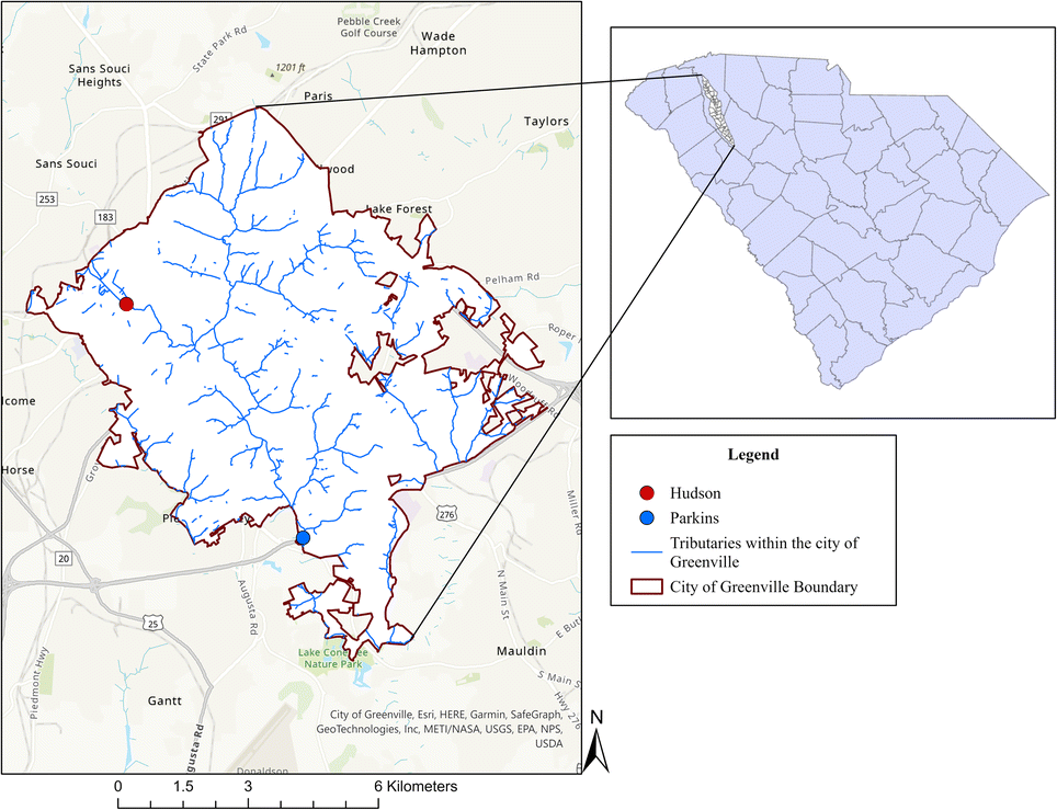 | ||
| Fig. 2 Greenville County's water quality monitoring network in upstate South Carolina, USA. | ||
Results and discussions
The results from the synthesis of over two dozen research articles are assimilated in the below section. The synthesis indicated the impacts of turbidity on aquatic ecosystems. To understand and conceptualize turbidity, the review is summarized and presented in Table 1. The scientific articles indicated various factors that contributed to turbidity such as forest fire, sedimentation, erosion, etc. The studies indicated the impact of urbanization, agriculture, deforestation and other human and climate-induced changes on turbidity. While in general, hydrology impacted turbidity through various processes such as erosion, turbidity influenced various ecological processes and characteristics in aquatic ecosystems such as predation vulnerability, food chain, photosynthesis, etc.| H, E, G, D and I categories | Citations |
|---|---|
| HD | Hjulstrom, 1935 (ref. 45) |
| • A forest fire and volcanic eruptions | Jackson and Starrett, 1959 (ref. 47) |
| • Sedimentation | Grayson et al., 1995 (ref. 48) |
| • Erosion of land | Haggard et al., 2001 (ref. 35) |
| • Erosion of stream bank | Sun et al., 2001 (ref. 49) |
| • Sediment resuspension | Sahoo et al., 2002 (ref. 34) |
| • Sanitary sewer overflows | Roy et al., 2003 (ref. 50) |
| • Nutrient concerns | Jin-liang et al., 2007 (ref. 51) |
| • Pollutant loadings | Peters et al., 2009 (ref. 37) |
| • Stream health | Huey and Meyer, 2010 (ref. 52) |
| Lin et al., 2011 (ref. 46) | |
| Eder et al., 2014 (ref. 41) | |
| Wang et al., 2014 (ref. 53) | |
| Guo et al., 2017 (ref. 38) | |
| Arnold and Toran, 2018 (ref. 40) | |
| Murphy et al., 2018 (ref. 43) | |
| Dar, 2019 (ref. 44) | |
| McMahon et al., 2020 (ref. 54) | |
| HI | DiSalvo et al., 1977 (ref. 55) |
| • Nutrient level | Starkey and Karr, 1984 (ref. 56) |
| Lloyd et al., 1987 (ref. 57) | |
| • Attached are pollutants such as oil and grease, and pesticides | Boxall and Maltby, 1995 (ref. 29) |
| • Stream productivity | Dolgonosov and Korchagin, 2003 (ref. 58) |
| • Dissolved oxygen level | Murphy et al., 2018 (ref. 43) |
| • Intakes of water supply | Villa et al., 2019 (ref. 59) |
| USGS, 2020 (ref. 42) | |
| Lenstra, et al. 2022 (ref. 28) | |
| ED | Bhargava and Mariam, 1990 (ref. 60) |
| • Light penetration | Kim et al., 2001 (ref. 61) |
| • Eutrophication | |
| EI | Abrahams and Kattenfeld, 1997 (ref. 62) |
| • Predation dynamics | Jarvenpaa and Lindstorm, 2004 (ref. 39) |
| • Predation vulnerability | |
| • Recruitment | |
| • Impacts oxygen level | |
| • Algal growth | |
| G | Wang et al., 2010 (ref. 63) |
| • Negative aesthetic and recreational appeal | Österling et al., 2010 (ref. 33) |
| E | Holbrook et al. 2013 (ref. 32) |
| • Biodiversity | USGS, 2020 (ref. 42) |
| • Control of populations of aquatic organisms (including macro-invertebrates and lotic food webs) | |
| D | |
| • Interfere with the ability for higher organisms to graze | |
| • Reductions in primary productivity due to increased light attenuation limit food available for secondary production | |
| I | |
| • Increasing water treatment costs | |
| NC | |
| • Suspended matter instrumentally controls the reactivity, transport and biological impacts of substances in aquatic environments, and provides a crucial link for chemical constituents between the water column, bed sediment and food chain | |
| HD | |
| • Turbidity variation affecting water quality | |
| EI | Vinçon-Leite and Casenave, (2019)64 |
| • Lake eutrophication, hypoxia, anoxia, and loss of biodiversity due to nutrient loading | |
| • The proliferation of primary producers (phytoplankton, aquatic plants, cyanobacteria) | |
| DH | Fournier et al. (2007)30 |
| • In karst, hydro systems are used as natural tracers for providing hydrodynamic information | Jafar-Sidik et al. 2017 (ref. 31) |
| • Understanding and characterizing transport properties of dissolved elements (surface water geochemistry) and particulate matter transport | |
| • Used in the vulnerability of karst aquifer vulnerability assessment to nitrates and phosphate contamination | |
| DE | Borok 10-WQ-022 – Oregon water quality65 |
| • Aquatic life | |
| • Reduced primary production and cascading effects on higher trophic levels | |
| • Effects on fish prey-predator dynamics and subsequent growth effects | |
| • Recreation | |
| • Swimming and aesthetics | |
| • Domestic water supply | |
| THE | Kitchener et al. (2017)66 |
| • Turbidity measurement as a surrogate typically suspended sediment concentration (SSC) or total suspended solids (TSS) | |
| ED | |
| • Reduction of visual range in water (affecting the ability of predators to hunt) | |
| • Photosynthesis | |
| HD | |
| • Sediment-transport processes | |
| DE | Osterling et al. (2010)33 |
| • Habitat degradation, population decline, species extinction, host-parasite relationship | |
| • Impact benthic, filter-feeding organisms through changes in their foraging activity and growth, clogging of interstitial spaces may also negatively affect the development of embryos of the mussel's salmonid host, which incubates its eggs in the gravel, recruitment | |
| IE | |
| • Habitat degradation, population decline, species extinction, species life span changes | |
| • Growth rate, age at maturity, mobility, and foraging mode | |
| NC-E | Ward et al. (2016)26 |
| • Predation vulnerability of introduced species and native species | |
| HD | Huey and Meyer (2010)52 |
| • Indicator of TSS, E. coli and Enterococci spp. | |
| HD | White et al. (2006)27 |
| • Disruptions to the water supply | |
| HI | |
| • This resulted in the construction of a major water filtration plant to address turbidity and water quality issues |
Since turbidity can shape many hydrological and ecological processes, directly or indirectly, once the summary of the articles was synthesized in Table 1 based on different categories (e.g., H, E, G, D, and I), the articles were further reorganized and presented in Table 2 based on combinations such as HD, HI, ED, and EI, to enhance clarity, facilitate better analysis and understanding of the interplay between turbidity and its impacts on the studied processes.
| HD | HI | ED | EI |
|---|---|---|---|
| • Hjulstrom, 1935 (ref. 45) | • DiSalvo et al., 1977 (ref. 55) | • Bhargava and Mariam, 1990 (ref. 60) | • Abrahams and Kattenfeld, 1997 (ref. 62) |
| • Jackson and Starrett, 1959 (ref. 47) | • Starkey and Karr, 1984 (ref. 56) | • Kim et al., 2001 (ref. 61) | • Järvenpää and Lindström, 2004 (ref. 39) |
| • Grayson et al., 1995 (ref. 48) | • Lloyd et al., 1987 (ref. 57) | • Borok 10-WQ-022-Oregon Water Quality65 | • Vincon-Leite and Casenave, 2019 (ref. 64) |
| • Haggard et al., 2001 (ref. 35) | • Boxall and Maltby, 1995 (ref. 29) | • Kitchener et al., 2017 (ref. 66) | |
| • Sun et al., 2001 (ref. 49) | • Dolgonosov and Korchagin, 2003 (ref. 58) | • Osterling et al., 2010 (ref. 33) | |
| • Sahoo et al., 2002 (ref. 34) | • Osterling et al., 2010 (ref. 33) | ||
| • Roy et al., 2003 (ref. 50) | • Murphy et al., 2018 (ref. 43) | ||
| • White et al., 2006 (ref. 27) | • USGS, 2020 (ref. 42) | ||
| • Fournier et al., 2007 (ref. 30) | • Lenstra, et al. 2022 (ref. 28) | ||
| • Kitchener et al., 2017 (ref. 66) | |||
| • Jin-liang et al., 2007 (ref. 51) | |||
| • Peters et al., 2009 (ref. 37) | |||
| • Huey and Meyer, 2010 (ref. 52) | |||
| • Wang et al., 2010 (ref. 53) | |||
| • Lin et al., 2011 (ref. 46) | |||
| • Eder et al., 2014 (ref. 41) | |||
| • Wang et al., 2014 (ref. 53) | |||
| • Guo et al., 2017 (ref. 38) | |||
| • Arnold and Toran, 2018 (ref. 40) | |||
| • Murphy et al., 2018 (ref. 43) | |||
| • Dar, 2019 (ref. 44) | |||
| • McMahon et al., 2020 (ref. 54) |
Hydrology–turbidity–ecosystem interactions (step 1)
The potential broad causes of the presence of suspended particulates and inorganic materials in the aquatic ecosystem are human, animal and nature-induced (Table 1). For example, land disturbances and changes caused by humans and animals, unmanaged construction activities, agricultural and grazing activities, timber harvesting, algae and phytoplankton in the system, instream processes, natural events (fire, volcanos), stream gradient, geology, discharges from wastewater, sanitary sewer, combined sewer overflows, etc. cause alteration of turbidity and likely suspended sediment concentration in the waterbodies. These causes influence the levels of turbidity in an aquatic ecosystem.26,27 Sediment inflows into reservoirs lead to water quality problems, particularly concerning turbidity.27 While the causes of turbidity are human, animal, or natural, some of the characteristics and processes behind the causes of turbidity are land (e.g., watershed processes), water (e.g., in-stream and in-lake processes) and atmosphere based (e.g., hurricane and rainfall processes) Additionally, some combination of these processes (e.g., fire). Turbidity shapes several ecological and hydrological processes directly and indirectly.Turbidity is one of the principal water quality parameters of concern for domestic water supplies.27 Because turbidity is caused by sediment, removal of the sediment from water supplies becomes important. Turbidity caused by sediment brings in several pollutants that are attached to the sediment surface. Oil and grease, metals, and pesticides to name a few that come with sediment.28,29 These attached pollutants are eliminated from the water supply to meet the permit compliance and regulations. Turbidity can serve as one of the natural tracers for characterizing dissolved elements (surface water geochemistry) and suspended particulate matter transport.30,31 Characteristics of particulate matter impact turbidity.
Suspended matter impacts sediment transport and various biogeochemical processes in surface waters. Even small changes in turbidity may be sufficient to alter predation dynamics, by impacting the way visual predators (e.g., trout) detect prey using contrast, while on the other hand, it impacts the ability of species (e.g., endangered humpback).32 Turbidity would likely reduce age, and lake trout intake rates given that foraging experiments on adult lake trout have found a reduction in reaction distances with increasing turbidity. Therefore, turbidity is an important parameter used in predation vulnerability studies which is important when evaluating management options for the preservation of native species (e.g., fishes).25 Turbidity degrades stream habitats and may negatively impact benthic, filter-feeding organisms (e.g., mussels) through reduced foraging activity both growths directly and indirectly.33 Turbidity directly clogs the intestinal spaces in mussels which also affects the development of embryos of the mussel's salmonid host, which incubates its eggs in the gravel. Reduced trout embryos are indirectly affected by mussel recruitment.33 Recruitment (addition of new individuals to populations) is a fundamental process in population dynamics that is impacted by turbidity. For example, recruitment is the linkage between spawning biomass (numbers and position of adults which breed) and new entrants into the population from eggs and larvae that adults deposit. Turbidity impacts predation vulnerability. For example, low turbidity (25 formazin nephelometric units) significantly reduced the predation vulnerability of bonytail to rainbow trout and led to a 36% mean increase in survival (24–60%, 95% CI) compared to trials conducted in clear water.25
Turbidity can indirectly shape several processes as well. Sedimentation and turbidity may also be positively correlated with nutrient levels, which can be associated with increased oxygen consumption and/or have toxic effects on the mussels, resulting in reduced survival of both juvenile and adult mussels.33 A positive relationship between species characteristics (e.g., trout density) and turbidity, may reflect differences in stream productivity.33 Studies have indicated that phosphorus binds well with sediment.34,35 Measuring and quantifying turbidity help in quantifying sediment-bound phosphorus. Phosphorus is one of the limiting nutrients for algal growth in lake systems. Quantification of the fate of phosphorus assists in understanding algal mechanisms in lake systems.
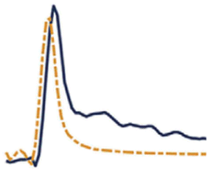
Land disturbances such as urbanization, unmanaged construction activities, timber production, agriculture, and grazing activities impact turbidity in a waterbody as described earlier. Urbanization including light and heavy industry, and urban and suburban development disturbs land and exposes soil.36–38 During rainfall events, the exposed soil erodes and makes its way to the waterbody increasing the turbidity of the water system, if not routed through a best management practice (BMP). Similarly, different types of agricultural activities (e.g., row crops, cover crops, silviculture, livestock grazing), agricultural operations (e.g., tillage, no-tillage) and irrigation management impact erosion and sediment movement to the surface water. This agricultural management and practices contribute to elevated turbidity if appropriate BMPs are not implemented. An example of rainfall and turbidity from the Reedy River watershed is shown in Fig. 3. The figure indicates the influence of rainfall on turbidity. Depending on the land use, generally, turbidity increases with the increase in rainfall.
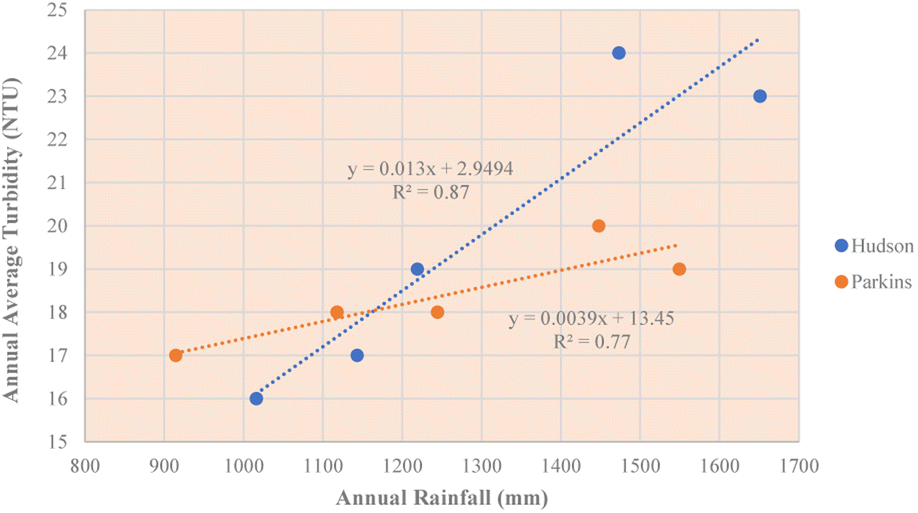 | ||
| Fig. 3 Example of rainfall and turbidity for different watersheds in the Reedy River Watershed, South Carolina. | ||
Turbidity and the algal growth process are interrelated. Algal growth needs light in aquatic ecosystems. Turbid water, either due to sediment or particulate matter, impacts light penetration limiting algal growth. On the contrary, algal growth by itself could impact the turbidity of the water. The impact of water turbidity due to algal growth could affect the mating system and the selection intensity.39
Various instream processes such as bank erosion, and resuspension of the bed sediment to the water column impact the turbidity in the water system. Bank erosion occurs due to a decrease in vegetation density in the riparian area coupled with elevated flows in the channel.40 It contributes soil particles to the water system causing increased turbidity in the stream. Resuspension of streambed sediments to the water column occurs due to stream flows that cause elevated turbidity.41 The dynamics of the particles in the bed change in different flow regimes. The sheer force of the flow in the stream causes the movement of the particle from the riverbed to the water column impacting turbidity. The process is dominant in streams and rivers and less common in lakes.
Natural processes such as volcanic eruptions and forest fires could contribute to turbidity. Volcanic ashfalls with finer particles could increase turbidity if they remain suspended in the water column. It impacts the water supply by clogging and damaging the filters at the intake of the treatment plant causing a financial burden to the treatment facility.42 Wildfires can lead to changes in the landscape. Runoff from a fire contains ash, which increases turbidity in the water system.43 Forest fire exposes the soil which could result in sediment load to the streams and lakes. Increased sediment load to these water systems increases turbidity and shortens the reservoir's lifetime. Rainfall impacts the turbidity of the water body through processes such as soil erosion. Soil erosion in the landscape, depending on the type of land use, could impact the sediment loadings in the waterbody.
Stream slopes or gradients impact the flow of water, and the flow of water impacts the movement of particles in the streams that influences turbidity. Different flow regimes have different carrying capacities of the sediment and the amount of sediment impacts the turbidity.44,45 The flow regimes could be natural or influenced by various land-use changes such as urbanization, development, agriculture etc. Geology and geologic disturbances play a vital role and are natural contributors to the level of turbidity in streams, rivers and lakes. The types of geologic materials in the drainage area affect the turbidity, directly or indirectly. Geologic disturbances such as earthquakes, and geologic or rainfall-induced landslides deliver a huge amount of sediment into the catchment.46
Sanitary sewer carries all sewage and wastewater from their designated sewer sheds, and combined sewer carries domestic sewage, industrial wastewater, and rainwater in one system. Overflows from these systems occur due to weather conditions such as heavy rainfalls. Due to leaks, lack of maintenance and other issues overflows contribute to an increase in turbidity in the waterways. The increase could adversely impact aquatic habitat, recreational value, and ecosystem services.
The results in Table 2 illustrated that compared to the processes related to hydrology, the processes on ecology are better documented for turbidity. Most studies have focused on the direct impacts from hydrology while fewer studies have focused on the indirect impacts on the ecological process in the context of turbidity. The findings from Table 2 highlight the need to further examine the indirect impacts of turbidity on ecological processes.
Turbidity drivers, causes, & SDGs (step 2)
Turbidity is conceptualized in relationship with SDGs through the drivers of interactions both directly and indirectly between various hydrological and ecological processes. Various drivers of turbidity are discussed and summarized from the literature. The linkage between drivers of turbidity and SDGs brings up various environmental implications discussed below.SDG 2-(Food)-agricultural or food production without good soil and water conservation practices (BMPs) can lead to soil erosion that would increase turbidity.67 Loss of soil through soil erosion reduces available topsoil for agriculture which could affect production.
SDG 7-(Energy)-ash is the by-product of coal production and is stored in ash ponds.68 Leaching of fly ash through fly ash ponds or accidental pond breaches could impact the turbidity in the river. The particle sizes of the riverbed could also change. Because of the size of the fly ash, the finer particles could block the sand bed and could reduce the interactions between the surface water and groundwater.
Demand for land to grow corn so that more energy crops and energy can be produced has increased significantly. This has resulted in the clearing of the land to develop bioenergy farms.67,68 Bioenergy agricultural production without good conservation practices (BMPs) can lead to increased turbidity in aquatic systems.68
SDG 11-(Cities)-land use change without the implementation of BMPs can cause erosion and an increase in turbidity.49,54,67 Vegetation in the riparian corridor could reduce bank erosion and help improve water quality. Land-use changes such as urbanization impact turbidity. BMPs are important to reduce the level of TSS and turbidity. Reduction in turbidity could help in developing sustainable cities. The study found that large storms dominate erosion in the catchment. The erosion rate depends on peak storm flow more than other hydrological variables. Combined sewer overflows.69 Sewer sediments could potentially increase turbidity in the watershed. They found that during rain events, the eroded fluxes are very important than the whole sewer sediment accumulated during the non-storm events.
SDG 13-(Climate)-changes in precipitation patterns (e.g., intense storms) can influence turbidity.49 The rate of erosion and rate of turbidity depends on peak storm flow in the watershed. Volcanic eruptions and forest fires lead to ashes which increased turbidity when rainfall washes the ashes away to the river and streams.52
SDG 14-(Life below water)-Flora decay and fauna feeding/excrement cause turbidity in lotic and lentic systems.62 Turbid waters could make a very productive aquatic ecosystem. They help in predation. For fish, turbidity will reduce the distance at which predation–prey interactions occur. The research indicated that the impact of predation risk will be reduced in the turbid aquatic ecosystem.
SDG 15-(Life on land)-cattle crossing causes land disturbances which impact turbidity in streams.70 The study indicated the impact of the herd of dairy cows crossing streams. They produce a plume of sediment, turbidity and high faecal coliform concentrations. When the cows wandered as individuals or small groups, the turbidity was minimal.
Turbidity impacts & SDGs (step 2)
Turbidity is conceptualized in relationship with SDGs through direct and indirect impacts on various hydrological and ecological processes. The impacts of turbidity are discussed and summarized from the literature. The linkage between the impact of turbidity and SDGs brings up various environmental implications discussed below.SDG 3-(Well-being)-consumption of turbid water impacts the health of livestock and human.71 Water quality impact due to turbidity demonstrated that aquatic life and water use for domestic purposes were not suitable. Various diseases associated with turbidity were also marked in this study.
SDG 5-(Gender equality)-when women are responsible for cleaning at home, turbid water increases their burden for processing water (e.g., boiling, filtering).72 The study found that water boiled in Guatemala was a common way to treat water in the home. Turbid water increases the effort of boiling and cleaning. Females in these countries are responsible for household chores. Turbid water increases their household chore time.
SDG 6-(Freshwater)-turbid water impacts the physical, chemical, and biological (bio-physicochemical) integrity of the aquatic system.57 The authors found that primary production decreased in shallow interior Alaskan streams caused by sediment-induced turbidity. This affected the bio-physiochemical integrity of the aquatic system.
SDG 7-(Energy)-hydropower generation with turbid water could lead to the clogging of turbines.73 The study found that sediment-laden rivers and reservoirs cause hydro-abrasive erosion in the turbines which is an important economic issue for power plant generation. Sediment load can be reduced to have less impact on the turbine. Maybe the turbine could be switched off during high turbid load. Turbid water in reservoir-diminishing reservoir capacity causes reduced head-impact hydropower generation.74 Society depends on reservoirs to get water, electricity, and recreational services. With diminishing capacity, all these services are minimized and compromised.
SDG 8-(Economic growth)-turbid water could lead to an increase in the clean-up cost.75 The authors found that the treatment cost of water increases with an increase in turbidity. This affects the cost of water and the availability of water to the community. It's a financial burden to the community and society.
SDG 10-(Inequalities)-turbid waters increase water purification and cleaning cost. It impacts economically vulnerable communities.75 Poor depends on the water either provided by the government or from natural sources. Since turbid water increases the cost of water, it affects the livelihood of the poor more than the rich. Clean and purified water is less affordable for the poor. Inequalities increase in those conditions.
SDG 11-(Cities)-turbid water decreases the drinking water availability from dams/reservoirs. It increases the water treatment cost.76 It also affects the aesthetics of the streams and rivers located in the urban area.
SDG 14-(Life below water)-turbid water affects species richness and biodiversity in various aquatic ecosystems.62,76
SDG 15-(Life on land)-turbid water affect species richness and biodiversity.62
The outcomes of the analysis of the relationship between turbidity, SDGs and targets are visually presented and summarized in Fig. 4 and 5. SDGs 2, 3, 5, 6, 7, 8, 10, 13, 14, and 15 linked to drivers and impacts of turbidity have 102 targets (Fig. 5). Among the 102 targets, 26 targets are of high relevance, 23 targets are of medium relevance, 24 targets are of low relevance, and the rest have no relevance to turbidity.
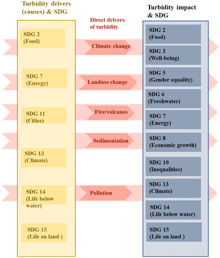 | ||
| Fig. 4 Conceptualization of Drivers and Impacts of turbidity as it relates to SDGs. | ||
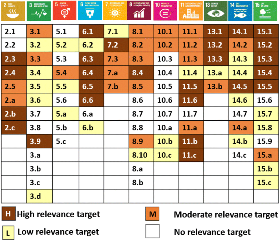 | ||
| Fig. 5 SDGs and their targets that drive and/or impact turbidity. The SDG icons are courtesy of UN SDG. | ||
Turbidity hysteresis and SDGs (step 3)
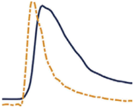
With an understanding that turbidity is impacted by various watershed processes such as land-use change, land disturbances, stream bank erosion, wash load, first flush, and rainfall, a hysteresis analysis helps in understanding these key watershed processes, so that preventive measures can be taken to improve the health of the watershed (Table 3, columns 1 to 4). Three types of hysteresis could occur-no hysteresis (row 1 of Table 3), clockwise positive hysteresis (rows 2, 3, 4 of Table 3), and anticlockwise negative hysteresis (row 5 of Table 3) which helps in understanding watershed disturbances and developments. No hysteresis, clockwise positive hysteresis, and anticlockwise negative hysteresis were adapted from Hamshaw et al., (2018)24 and the processes influencing the hysteresis pattern were adapted from Malutta et al., (2020).25 This study innovatively developed the relationship between columns 1 through 4 and SDGs (column 5 of Table 3) and their relationship with SDGs.| PDF between flow and turbidity | Hysteresis | Class (description of the PDF and hysteresis) | Different processes | SDGs |
|---|---|---|---|---|
|

|
Class I: no hysteresis, the peak of turbidity matches the peak of flow | Sediment discharge and flow time are equal travel time, an abundance of fine sediments in the channel, low availability of fine-grained sediment, abundant supply of sediment/mobilization of sediment in the channel, followed by the transport from the distant source within the watershed | |
|

|
Class II: clockwise, positive hysteresis, the peak of turbidity leads to the peak of flow | Local sediment sources such as in-channel sediment, close-by sediment, bank loss, exhaustion of sediment after the initial flush, formation of the armoured layer before peak discharge, increased baseflow after peak discharge leading to dilution of sediment concentration, runoff events from snowmelt, wash load, early sediment load from tributaries | SDG 2 and 11 |
|

|
Class II: clockwise, positive hysteresis, the peak of turbidity leads to the peak of flow | The turbidity responses are peak, leading the hydrograph however, the peak decreased abruptly, indicating that the local source contributed initially, but then over time, the regional source contributed less to the overall hydrograph, maybe the watershed is very impervious with little source of turbidity in the watershed | SDG 2 and 11 |
|

|
Class II: clockwise, positive hysteresis, the peak of turbidity leads to the peak of flow | The turbidity peaks before the flow drop off pretty sharply, however, the baseflow and the recession limb continue to stretch a bit which could be due to increased baseflow after the peak discharge leading to the dilution of the sediment, which is possibly due to elevated groundwater and interflow. This could also be possible in short near channel sources, early sediment supply by the tributaries and loss of sediment from the tributaries, usually in smaller basins | SDG 11 |
|

|
Class III: counter clockwise, negative hysteresis, the peak of turbidity lags the peak of flow | Sediment wave travels slower than the discharge in general, high soil erodibility, bed/bank erosion, distant sediment source, late sediment supply by tributaries, exhaustion of sediment available due to the previous event, seasonality (lower concentrations early in the year), valley slopes are important sediment source, non-uniform sediment distribution, small evens with high rainfall intensity and very dry soil, channel deposition, the influence of sea tide on hysteresis, landslide, very high moisture and high antecedent rainfall conditions | SDG 2, 7, 11 and 13 |
Example application to the Reedy River Watershed (step 4)
Results from the turbidity data obtained from Hudson and Parkins in the Reedy River is discussed based on conceptualization, its relationship with SDGs and various key analysis such as hysteresis, cumulative frequency plots, flow-based turbidity analysis.On average, Hudson and Parkins marked 24 and 20 NTUs for the year 2013–2014, and 19 and 18 NTUs for the year 2014–2015, respectively. While Hudson experienced rainfall of 58 inches in the year 2013–2014, Parkins experienced 57 inches in the same year. In the year 2014–2015, Hudson marked a rainfall of 48 inches, and Parkins marked 49 inches. Because both the sites marked more rainfall during the year 2013–2014 compared to 2014–2015, turbidity was higher in that year at both the sites compared to the year 2014–2015. In general, the downstream of the city produced less average annual turbidity indicating that the matured urban growth could have less opportunity for elevated turbidity in the aquatic ecosystem. It could also be that the stormwater BMPs implemented in the urban areas helped reduce the sediment load to the downstream waterbodies.
Hysteresis analysis indicated several observations. Table 4 shows average hysteresis index values for the storms analyzed in 2013–2014 and 2014–2015. On average, annually, both the sites marked negative hysteresis except in 2013–2014, where Hudson marked positive hysteresis. Negative hysteresis occurs when peak flow leads the peak turbidity. This property could be classified as class III counterclockwise negative hysteresis (Table 3). In this type of hysteresis, the sediment wave travels slower than the discharge in general. Under this category, various SDGs such as 11 and 13 can be considered. In general, the analysis indicated a large negative hysteresis at the Parkins in both the years, 2013–2014 and 2014–2015. This station had 10 negative hysteresis index results produced from the 12 analyzed storm events in 2013–2014 and 11 negative hysteresis indexes from 12 analyzed storms in 2014–2015. This station captures runoff from the highly developed area of the City of Greenville. Areas with a higher percentage of impervious areas have been associated with lower turbidity readings. Given that Parkins is situated in a highly urbanized area, little sediment is likely contributed to the river from local runoff, keeping the turbidity in the leading limb of the hydrograph lower than the turbidity in the falling limb of the hydrograph, when sediment from the more rural area in the northern part of the watershed is moving past the station. Immediately upstream of the station is located a tributary that drains an impoundment (Fig. 6, E. P. Collins Lake Dam), which might be causing the delay in turbidity flux, causing the negative hysteresis at Parkins. Negative hysteresis could be because the urban stormwater ponds that retain water and help in settling the sediment, could be working well. Stormwater ponds slow down the movement of sediment and flow downstream. Immediate upstream of both locations is located tributaries. They might be contributing to the late sediment supply to the streams causing negative hysteresis. A small negative hysteresis at Hudson in 2014–2015, could be due to some distant source contributing to the turbidity. The watershed is rural by nature and has forest cover. This could be a contributing factor, where turbidity is much delayed.
| 2013–2014 | 2014–2015 | ||||
|---|---|---|---|---|---|
| Hudson | Parkins | Hudson | Parkins | ||
| Jul-13 | 0.51 | −9.85 | Jul-14 | −0.63 | −15.91 |
| Aug-13 | −0.78 | −6.30 | Aug-14 | −0.52 | −10.40 |
| Sep-13 | 0.33 | −2.01 | Sep-14 | 0.70 | −3.50 |
| Oct-13 | 1.15 | −1.75 | Oct-14 | 0.22 | −8.02 |
| Nov-13 | 0.37 | −0.77 | Nov-14 | −0.20 | −0.43 |
| Dec-13 | 0.80 | 0.61 | Dec-14 | 0.35 | 0.20 |
| Jan-14 | 0.01 | −0.60 | Jan-15 | −3.90 | −0.22 |
| Feb-14 | −0.39 | −1.04 | Feb-15 | −0.63 | −0.70 |
| Mar-14 | 0.93 | 0.29 | Mar-15 | 0.10 | −2.10 |
| Apr-14 | −0.06 | −0.70 | Apr-15 | 0.70 | −4.82 |
| May-14 | 0.20 | −13.48 | May-15 | 0.03 | −13.05 |
| Jun-14 | 0.81 | −4.56 | Jun-15 | 0.24 | −12.40 |
| Average | 0.32 | −3.35 | −0.29 | −5.90 | |
 | ||
| Fig. 6 The screenshot of the tributary upstream of Parkins draining an impoundment. | ||
On the contrary, Hudson, in general, marked a positive hysteresis that was obtained from 12 analyzed storms in 2013–2014 (Table 4). Positive hysteresis is caused when peak turbidity leads to peak flows. This property could be classified as class II clockwise positive hysteresis (Table 3). In this type of hysteresis, local sediment sources play a critical role to lead the hydrograph. SDGs 2 and 11 can be explained under this category. This watershed is very rural no impoundment was prominent to control flow and turbidity, and the immediate land use is dominated by urban areas, which could have contributed to the positive hysteresis at this site due to local sediment sources from the bank, or the nearby watershed. There could be some local sources from large tributaries upstream of the site contributing to the increase and peak of turbidity, resulting in positive hysteresis.
Turbidity cumulative frequency analysis (Fig. 7) indicated that Hudson, which is upstream of the City of Greenville, exceeded the 50 NTU limit approximately 15% of the time during the year 2013–2014, while turbidity at Parkins, which is below the City of Greenville, exceeded the 50 NTU limit approximately 10 percent of the time in the same year. The shape of the turbidity exceedance plots at both sites was similar for 2013–2014. In the year 2014–2015, the turbidity exceedance plots (Fig. 7) indicated that at both sites, turbidity exceeded the 50 NTU limit, approximately 10 percent of the time. Although the shape of the curves was similar throughout, the shape of the curves between 10% and 60% exceedance levels indicated that higher turbidity values were marked at Hudson in this zone. The higher-level exceedances indicated the impact of large storms on turbidity.
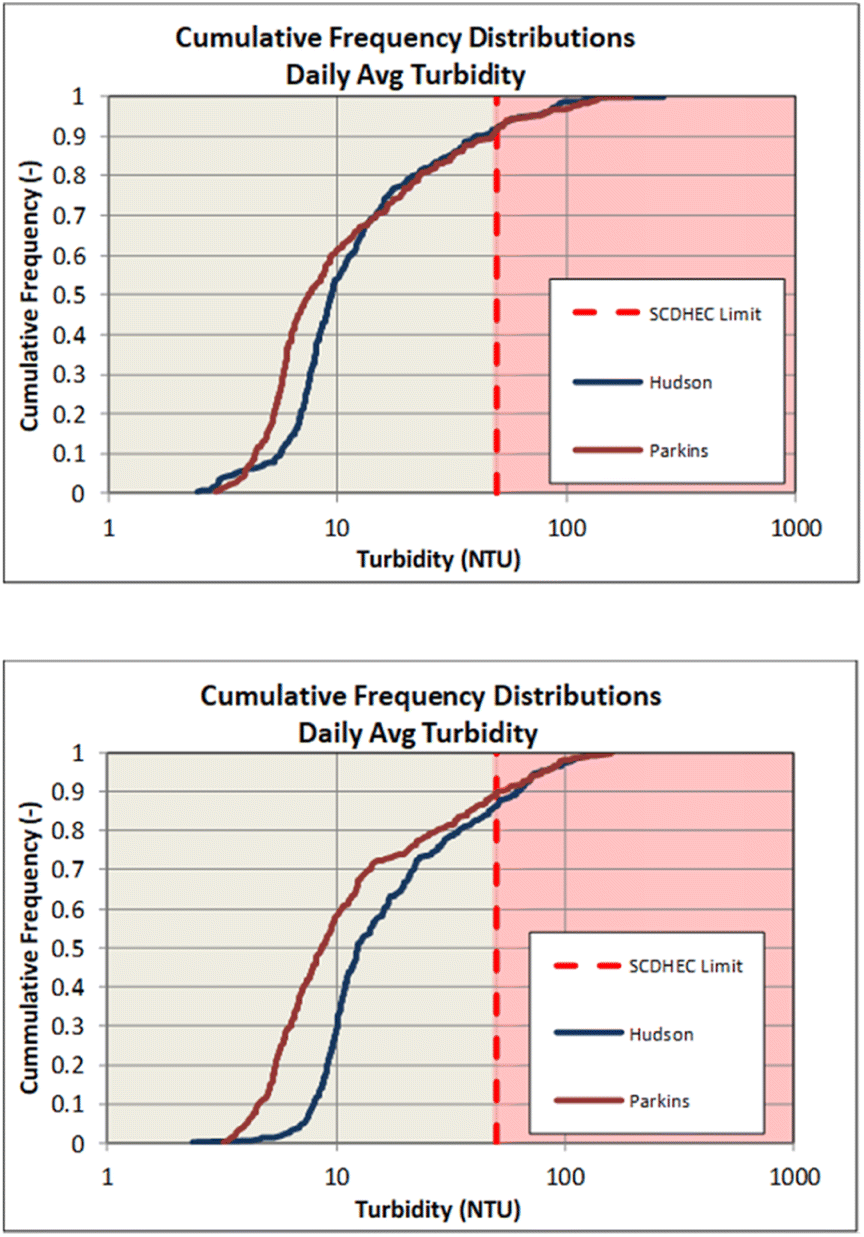 | ||
| Fig. 7 Cumulative daily average turbidity probability plots for the years 2013–2014 (top) and 2014–2015 (bottom). | ||
The flow-based turbidity graphs (Fig. 8) for both years indicated that the highest turbidity was marked in the top 10 percent of the flows at both sites. Following the top 10% of the flow, turbidity decreased rapidly and remained at low levels, below the 50 NTU standard, in all the flow regimes. The highest turbidity is due to high flows and corresponding rainfall. Other processes such as stream bank erosion, bed erosion, and watershed disturbances could have also influenced high turbidity. The mean turbidity in the top 10% of the flow category, was slightly lower at Hudson than at Parkins, indicating the possible influence of various watershed characteristics such as impervious area, urban development and erosive power of the stream at Parkins.
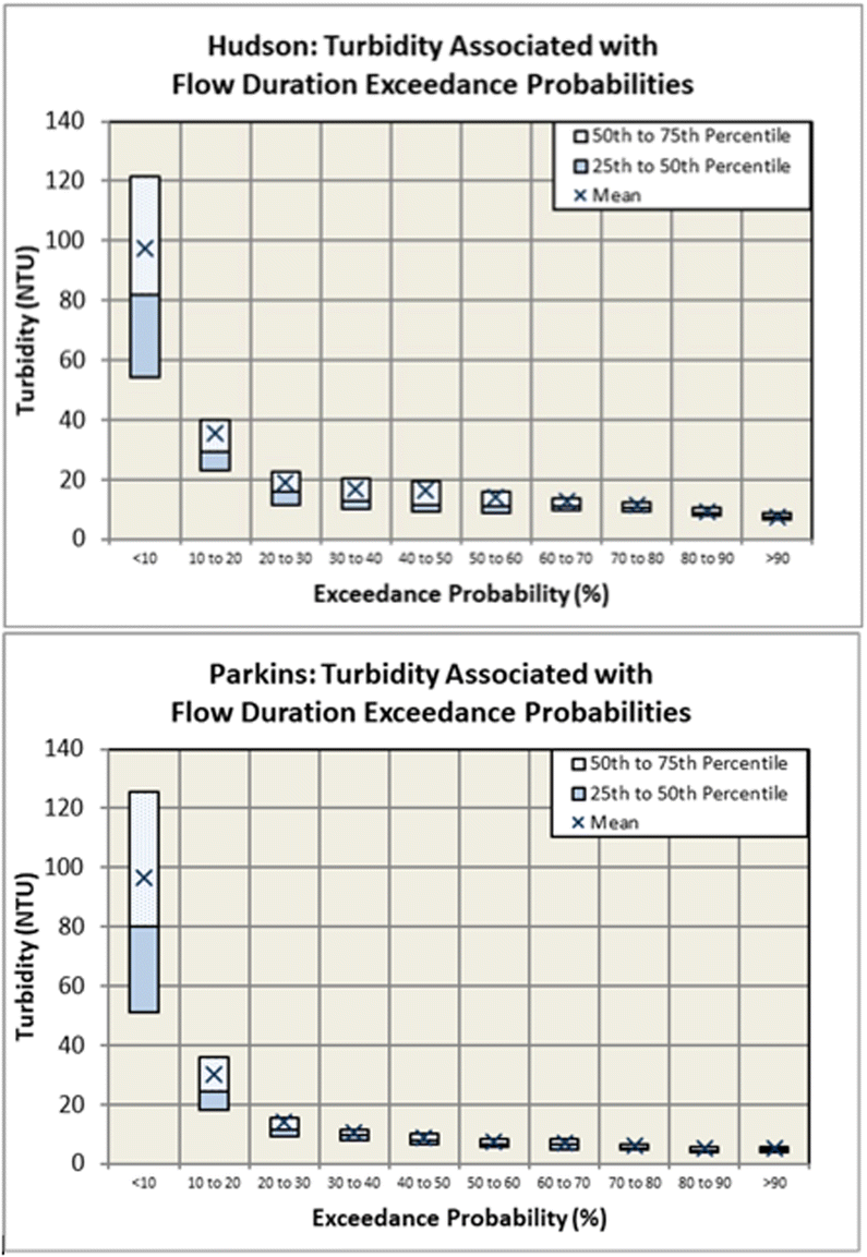 | ||
| Fig. 8 Flow-based turbidity for the year 2013–2014: Hudson (top) and Parkins (bottom). The graph for 2014–2015 is included as ESI Materials.† | ||
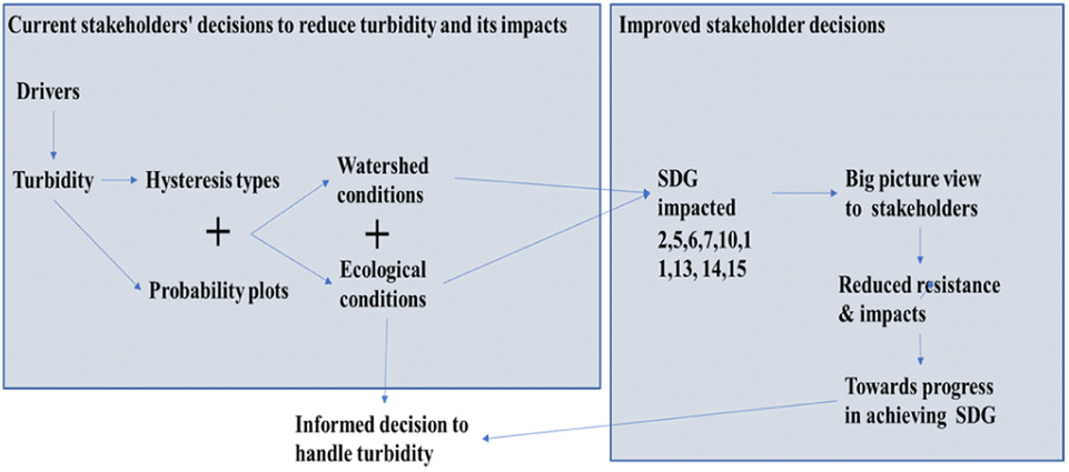
Support stakeholders in making informed decisions in managing turbidity
Stakeholders in the watershed such as wastewater plant managers and operators generally focus on reducing turbidity based on the regulatory standards and requirements set by the state and federal regulatory agencies. The current approach described in this article will provide the managers and operators with information beyond the traditional requirements on turbidity. An understanding of turbidity, the drivers of turbidity, the causes of turbidity, watershed and ecological conditions, their responses, and the relationship with SDGs will provide the bigger picture and could change the stakeholder's perception. The stakeholder's social perception of the different BMPs based on aesthetic and landscape benefits, acceptability, improvement to the quality of life and contributions to sustainable development can be improved. By taking into consideration the bigger picture and considering the holistic impacts of BMPs including their potential influence on economic performance, estimations, and cost analysis, there is an opportunity to drive significant change. Improving stakeholder perceptions and understanding of turbidity can lead to more informed decisions, optimized resource allocation, and better outcomes in terms of environmental sustainability, economic viability and social well-being, which are some of the purposes of UN SDGs.Expanding further, this context will enable the stakeholders such as city managers, county officials, farmers, homeowners, and home builders in taking proactive measures than reactive measures to reduce the impacts of turbidity (Fig. 7). Proactive measures to reduce turbidity in a watershed by understanding various factors that contribute to elevated turbidity would aid in better operations and management of treatment plants (Fig. 9).
 | ||
| Fig. 9 Connections and links showing turbidity and its association with SDGs and water resources research. | ||
Conclusions
The conceptualization of turbidity plays a pivotal role in conducting detailed research to gain a comprehensive understanding of turbidity, its drivers and its impacts on the hydrological and ecological systems. During this research various SDGs and their associated targets were identified and linked to turbidity, highlighting the environmental implications of turbidity within the context of SDGs. While the steps of conceptualization of turbidity can be applied universally, the identified goals and targets can be subjective to the chosen location. An analysis of turbidity data obtained from two monitoring sites in the Reedy River utilizing hysteresis and frequency plots revealed diverse watershed conditions and processes such as impact from urbanization, stormwater ponds, local sediment sources, distant sources, and their linkages to SDGs. The analysis also indicated the probability of high turbidity in the system and the percent time they were observed. While watershed stakeholders and managers often prioritize regulatory standards for turbidity to improve water quality, the current research equip them with a comprehensive understanding of turbidity across the entire landscape. The understanding equipes stakeholders with the knowledge needed to take informed decisions and actions aimed at improving turbidity in various waterbodies.Author contributions
D. Sahoo: conceptualization, methodology, investigation, writing – original draft preparation, data curation, project administration. A. Anandhi: conceptualization, methodology, writing – original draft preparation.Conflicts of interest
There are no conflicts to declare.Acknowledgements
The study was possible due to the data shared by the Reedy River 5R group. The authors would like to acknowledge Ibrahim Busari and Morolake Fatunmbi for their assistance in preparing this manuscript. Dr Anandhi would like to acknowledge the support from USDA-NIFA capacity building grants 2022-38821-37522, USDA-NIFA Evans-Allen Project, Grant 11979180/2016–01711, USDA-NIFA grant no. 2018–68002–27920, as well as National Science Foundation Grant No. 1735235 awarded as part of the National Science Foundation Research Traineeship and Grant No. 2123440.References
- M. Mannan, T. Al-Ansari, H. R. Mackey and S. G. Al-Ghamdi, Quantifying the energy, water, and food nexus: a review of the latest developments based on life-cycle assessment, J. Cleaner Prod., 2018, 193, 300–314 CrossRef.
- A. Mitra and N. Rao, Gender, water, and nutrition in India: an intersectional perspective, Water Altern., 2019, 12, 930–952 Search PubMed.
- L. Bizikova, D. Roy, D. Swanson, H. D. Venema and M. McCandless, The Water-Energy-Food Security Nexus: Towards a Practical Planning and Decision-Support Framework for Landscape Investment and Risk Management, International Institute for Sustainable Development, Winnipeg, 2013 Search PubMed.
- D. L. Keairns, R. C. Darton and A. Irabien, The Energy-Water-Food nexus, Annu. Rev. Chem. Biomol. Eng., 2016, 7, 239–262 CrossRef CAS PubMed.
- R. J. Davies-Colley and D. G. Smith, Turbidity suspended sediment and water clarity: a review, J. Am. Water Resour. Assoc., 2001, 37, 1085–1101 CrossRef.
- South Carolina Department of Health and Environmental Control (SCDHEC), Regulations 61-68 Water Classifications and Standards, 2014 Search PubMed.
- J. U. Grobbelaar, Turbidity, in Encyclopedia of Inland Waters, 2009 Search PubMed.
- Department of Environmental Quality, State of Oregon, Turbidity Technical Review, 2014 Search PubMed.
- USEPA National Primary Drinking Water Regulations, 2009 Search PubMed.
- H. Babaie, A. Davarpanah and N. Dhakal, Projecting pathways to Food-Energy-Water systems sustainability through ontology, Environ. Eng. Sci., 2019, 36, 808–818 CrossRef CAS.
- X. Chen, W. Chen, Y. Bai and X. Wen, Changes in turbidity and human activities along Haihe River Basin during lockdown of COVID-19 using satellite data, Environ. Sci. Pollut. Res., 2021, 1–16 Search PubMed.
- A. P. Yunus, Y. Masago and Y. Hijioka, COVID-19 and surface water quality: improved lake water quality during the lockdown, Sci. Total Environ., 2020, 731, 139012 CrossRef CAS PubMed.
- C. Carmona-Moreno, C. Dondeynaz and M. Biedler, Position Paper on Water, Energy, Food and Ecosystems (WEFE) Nexus and Sustainable Development Goals (SDGs), 2018 Search PubMed.
- S. Robinson, R. Brooks, K. Kotiadis and D. J. Van Der Zee, Conceptual Modeling for Discrete-Event Simulation, CRC Press, 2010 Search PubMed.
- A. Anandhi and N. Kannan, Vulnerability assessment of water resources–translating a theoretical concept to an operational framework using systems thinking approach in a changing climate: case study in Ogallala Aquifer, J. Hydrol., 2018, 557, 460–474 CrossRef.
- A. Anandhi and C. Bentley, Predicted 21st century climate variability in south eastern US using downscaled CMIP5 and meta-analysis, Catena, 2018, 170, 409–420 CrossRef.
- A. Anandhi and -A. CISTA, Conceptual model using indicators selected by systems thinking for adaptation strategies in a changing climate: a case study in agro-ecosystems, Ecol. Modell., 2017, 345, 41–55 CrossRef.
- J. Patrício, M. Elliott, K. Ma zik, K. N. Papadopoulou and C. J. Smith, DPSIR—two decades of trying to develop a unifying framework for marine environmental management?, Front. Mar. Sci., 2016, 3, 177 Search PubMed.
- C. Bentley and A. Anandhi, Representing driver-response complexity in ecosystems using an improved conceptual model, Ecol. Modell., 2020, 437, 109320 CrossRef.
- L. C. Stringer, C. Quinn, H. T. Le, F. Msuya, J. Pezzuti, M. Dallimer, S. Afionis, R. Berman, S. Orchard and M. Rijal, A new framework to enable equitable outcomes: resilience and nexus approaches combined, Earth's Future, 2018, 6, 902–918 CrossRef.
- J. Pagan, M. Pryor, R. Deepa, J. Grace III, O. Mbuya, R. Taylor, J. O. Dickson, V. Ibeanusi, A. Chauhan and G. Chen, Sustainable Development Tool Using Meta-Analysis and DPSIR Framework—Application to Savannah River Basin, US, J. Am. Water Resour. Assoc., 2020, 56, 1059–1082 CrossRef.
- S. Robinson, A Tutorial on Simulation Conceptual Modelling; 2017 Winter Simulation Conference (WSC), IEEE, 2017, pp. 565–579 Search PubMed.
- The National Graduate Institute for Policy Studies (GRIPS), UN Sustainable Development Goals: Blueprint for a Better Future, 2018 Search PubMed.
- S. D. Hamshaw, M. M. Dewoolkar, A. W. Schroth, B. C. Wemple and D. M. Rizzo, A new machine-learning approach for classifying hysteresis in suspended-sediment discharge relationship using high-frequency monitoring data, Water Resour. Res., 2018, 54, 4040–4058 CrossRef.
- S. Malutta, M. Kobiyama, P. L. B. Chaffe and N. B. Bonumá, Hysteresis analysis to quantify and qualify the sediment dynamics: state of the art, Water Sci. Technol., 2020, 81, 2471–2487 CrossRef PubMed.
- L. W. Ward, R. Morton-Starner and B. Vagge, Effects of turbidity on predation vulnerability of juvenile humpback chub to rainbow and brown trout, J. Fish Wildl. Manage., 2016, 7, 1–8 Search PubMed.
- I. White, A. Wade, M. Worthy, N. Mueller, T. Daniell and R. Wasson, The vulnerability of water catchments to bushfires: impacts of the January 2003 wildfires on the Australian Capital Territory, Aust. J. Water Resour., 2006, 10(2), 179–193 Search PubMed.
- W. K. Lenstra, N. A. G. M. v. Helmond, O. M. Zygadlowska, R. v. Zummeren, R. Witbaard and C. P. Slomp, Sediments as a source of iron, manganese, cobalt, and nickel to continental shelf waters (Louisiana, Guld of Mexico, Front. Mar. Sci., 2022, 9, 1–13 Search PubMed.
- A. B. A. Boxall and L. Maltby, The characterization and toxicity of sediment contaminated with road runoff, Water Res., 1995, 9, 2043–2050 CrossRef.
- M. Fournier, N. Massei, M. Bakalowicz, L. Dussart-Baptista, J. Rodet and J. P. Dupont, Using turbidity dynamics and geochemical variability as a tool for understanding the behavior and vulnerability of a karst aquifer, Hydrogeol. J., 2007, 15, 689–704 CrossRef CAS.
- M. Jafar-Sidik, F. Gohin, D. Bowers, J. Howrah and T. Hull, The relationship between suspended particulate matter and turbidity at a mooring station in a coastal environment: consequences for satellite derived products, Oceanologia, 2017, 59(3), 365–378 CrossRef.
- B. V. Holbrook, T. R. Hrabik, D. K. Branstrator and A. F. Mensinger, Foraging mechanisms of age-0 lake trout (Salvelinus namaycush), J. Great Lakes Res., 2013, 39, 128–137 CrossRef.
- M. E. Österling, B. L. Arvidsson and L. A. Greenberg, Habitat degradation and the decline of the threatened mussel Margaritifera margaritifera: influence of turbidity and sedimentation on the mussel and its host, J. Appl. Ecol., 2010, 47, 759–768 CrossRef.
- D. Sahoo, I. Chaubey, B. Haggard, and M. Matlock, Stream nutrient dynamics and sediment nutrient interaction in an agricultural stream, Proceedings of American Society of Agricultural Engineers, Technical Meeting Paper No. 032281, 2003 Search PubMed.
- B. E. Haggard, D. E. Storm, R. D. Tejral, Y. A. Popova, V. G. Keworth and E. H. Stanley, Stream nutrient retention in three northeastern Oklahoma agricultural catchments, Trans. ASABE, 2001, 44(3), 597–605 CAS.
- D. M. Lawler, G. E. Petts, I. D. L. Foster and S. Harper, Turbidity dynamics during spring storm events in an urban headwater river system: The Upper Tame, West Midlands, UK, Sci. Total Environ., 2006, 360, 109–126 CrossRef CAS PubMed.
- D. P. Peters, J. R. Gosz and S. L. Collins, Boundary dynamics in landscapes, The Princeton Guide to Ecology, 2009, pp. 458–63 Search PubMed.
- X. Guo, T. Li, B. He and Y. Yao, Effects of land disturbance on runoff and sediment tield after natural rainfall events in southweatern China, Environ. Sci. Pollut. Res. Int., 2017, 24(10), 9259–9268 CrossRef PubMed.
- M. Järvenpää and K. Lindström, Water turbidity by algal blooms causes mating system breakdown in a shallow-water fish, the sand goby Pomatoschistus minutus, Proc. R. Soc. London, 2004, 271, 2361–2365 CrossRef PubMed.
- E. Arnold and L. Toran, Effects of bank vegetation and incision on erosion rates in an urban stream, Water, 2018, 10, 482 CrossRef.
- A. Eder, M. Exner-Kittridge, P. Strauss and G. BIöschl, Re-suspension of bed sediment in a small stream-results from two flushing experiments, Hydrol. Earth Syst. Sci., 2014, 18, 1043–1052 CrossRef.
- USGS, https://volcanoes.usgs.gov/volcanic_ash/water_supply.html, accessed on 12/20/2020.
- S. F. Murphy, R. B. McCleskey, D. A. Martin, J. H. Writer and B. A. Ebel, Fire, flood, and drought: extreme climate events alter flow paths and stream chemistry, J. Geophys. Res.: Biogeosci., 2018, 123, 2513–2526 CrossRef CAS.
- R. A. Dar, S. A. Mir and S. A. Romshoo, Influence of geomorphic and anthropogenic activities on channel morphology of river Jhelum in Kashmir valley, nw Himalayas, Quat. Int., 2019, 507, 333–341 CrossRef.
- F. Hjulstrom, Studies of the morphological activity of rivers as illustrated by the river Fyris, Bulletin of the Geological Institutions of the University of Uppsala, 1935, 25, 221–537 Search PubMed.
- J. Lin, M. Yang, B. Lin and P. Lin, Risk assessment of debris flows in Songhe Stream, Taiwan, Eng. Geol., 2011, 123, 100–112 CrossRef.
- O. H. Jackson and W. C. Starrett, Turbidity and sedimentation at lake Chautauqua, Illinois, J. Wildl. Manage., 1959, 23, 157–168 CrossRef.
- R. B. Grayson, B. L. Finlayson, C. J. Gippel and B. T. Hart, The potential of field turbidity measurements for the computation of total phosphorus and suspended solids loads, J. Environ. Manage., 1996, 47, 257–267 CrossRef.
- H. Sun, P. S. Cornish and T. M. Daniell, Turbidity-based erosion estimation in a catchment in South Australia, J. Hydrol., 2001, 253, 227–238 CrossRef.
- A. H. Roy, A. D. Rosemond, M. J. Paul, D. S. Leigh and J. B. Wallace, Stream macroinvertebrate response to catchment urbanization (Georgia, USA), Freshwater Biol., 2003, 48, 329–346 CrossRef.
- H. Jin-liang, D. U. Peng-fei, A. O. Chi-tan, L. E. I. Mui-heong, Z. Dong-quan, H. O. Man-him and W. Zhi-shi, Characterization of surface runoff from a subtropics urban catchment, J. Environ. Sci., 2007, 19, 148–152 CrossRef PubMed.
- G. M. Huey and M. L. Meyer, Turbidity as an indicator of water quality diverse watersheds of the Upper Pecos River basin, Water, 2010, 2, 273–284 CrossRef CAS.
- J. Wang, Combined sewer overflows (CSOs) impact on water quality and environmental ecosystem in the Harlem River, J. Environ. Prot., 2014, 5, 1373–1389 CrossRef CAS.
- J. M. McMahon, J. M. Olley, A. P. Brooks, J. C. R. Smart, B. Stewart-Koster, W. N. Venables, G. Curwen, J. Kemp, M. Stewart, N. Saxton, A. Haddadchi and J. C. Stout, Vegetation and longitudinal coarse sediment connectivity affect the ability of ecosystem restoration to reduce riverbank erosion and turbidity in drinking water, Sci. Total Environ., 2019, 707, 1–16 CrossRef PubMed.
- L. H. DiSalvo, H. E. Guard, N. D. Hirsch and J. Ng, Assessment and Significance of Sediment-Associated Oil and Grease in Aquatic Environments Final Report, 1977, pp. 1–146 Search PubMed.
- J. E. Starkey and P. R. Karr, Effect of low dissolved oxygen concentration on effluent turbidity, Water Pollut. Control Fed., J., 1984, 56, 837–843 CAS.
- D. S. Lloyd, J. P. Koenings and J. D. LaPerriere, Effects of turbidity in fresh waters of Alaska, N. Am. J. Fish. Manag., 1987, 7, 18–33 CrossRef.
- B. M. Dolgonosov and K. A. Korchagin, Statistical assessments of relationships between water flow in a river and water turbidity in water intakes, Water Resour., 2005, 32, 175–182 CrossRef CAS.
- A. Villa, J. Folster and K. Kyllmar, Determining suspended solids and total phosphorus from turbidity: comparison of high frequency sampling with conventional monitoring methods, Environ. Monit. Assess, 2019, 191, 605 CrossRef PubMed.
- D. S. Bhargava and D. W. Mariam, Light penetration depth, turbidity, and reflectance related relationships and models, J. Photogramm. Remote Sens., 1991, 46, 217–230 CrossRef.
- B. Kim, Ju-H. Park, G. Hwang, M.-S. Jun and K. Choi, Eutrophication of reservoirs in South Korea, Limnology, 2001, 2, 223–229 CrossRef CAS.
- M. Abrahams and M. Kattenfeld, The role of turbidity as a constraint on predator-prey interactions in aquatic environments, Behav. Ecol. Sociobiol, 1997, 40, 169–174 CrossRef.
- S. Wang, X. Qian and B. Han, Modeling the effects of inflow and outflow volume on turbidity variation in Liuxihe Reservoir, 4th International Conference on Bioinformatics and Biomedical Engineering, IEEE, 2010, pp. 1–4 Search PubMed.
- B. Vinçon-Leite and C. Casenave, Modelling eutrophication in lake ecosystem: A review, Sci. Total Environ., 2019, 651, 2985–3001 CrossRef PubMed.
- Oregon Department of Environmental Quality, Turbidity Technical Review: Summary of Sources, Effects, and Issues Related to Revisiting the State-wide Water Quality Standards for Turbidity, 2010 Search PubMed.
- B. G. B. Kitchener, J. Wainwright and A. J. Parsons, A review of the principles of turbidity measurements, Prog. Phys. Geogr., 2017, 41, 620–642 CrossRef.
- T. McDonald, G. D. Gann, J. Jonson and K. W. Dixon, International Standards for the Practice of Ecological Restoration-Including Principles and Key Concepts, Society of Ecological Restoration, 2016 Search PubMed.
- S. Pal, S. Mahato and S. Sarkar, Impact of fly ash on channel morphology and ambient water quality of Chandrabhaga River of Eastern India, Environ. Earth Sci., 2016, 75, 1268 CrossRef; J. E. Fargione, T. R. Cooper, D. J. Flaspohler, J. Hill, C. Lehman, T. McCoy, S. McLeod, E. J. Nelson, K. S. Oberhauser and D. Tilman, Bioenergy and wildlife: threats and opportunities for grassland conservation, BioScience, 2009, 59, 767–777 CrossRef.
- T. Bersinger, I. Hécho Le, G. Bareille and T. Pigot, Assessment of erosion and sedimentation dynamic in a combined sewer network using online turbidity monitoring, Water Sci. Technol., 2015, 1375–1382 CrossRef CAS PubMed.
- R. J. Davies-Colley, J. W. Nagels, R. A. Smith, R. G. Young and C. J. Phillips, Water quality impact of a dairy cow herd crossing a stream, N. Z. J. Mar. Freshwater Res., 2004, 38(4), 569–576 CrossRef.
- J. N. Halder and M. N. Islam, Water pollution and its impact on the human health, J. Hum. Environ., 2015, 2(1), 36–46 CrossRef.
- G. Rosa, L. Miller and T. Clasen, Microbiological effectiveness of disinfecting water by boiling in rural Guatemala, Am. J. Trop. Med. Hyg., 2010, 82, 473–477 CrossRef PubMed.
- D. Felix, I. Albayrak, A. Abgottspon and R. M. Boes, Optimization of hydropower plants with respect to fine sediment focusing on turbine switch-offs during floods, IOP Conference Series: Earth and Environmental Science, 2016 Search PubMed.
- J. P. C. Podolak and M. W. Doyle, Reservoir sedimentation and storage capacity in the United State: management needs for the 21st century, J. Hydraul. Eng., 2015, 141(4), 1–5 CrossRef.
- K. B. Shrestha, B. R. Thapa, Y. Aihara, S. Shrestha, A. P. Bhattarai, N. Bista, F. Kazama and J. Shindo, Hidden cost of drinking water treatment and its relation with socioeconomic status in Nepalese urban context, Water, 2018, 10, 607 CrossRef.
- S. W. Chung, M. R. Hipsey and J. Imberger, Modelling the propagation of turbid density inflows into a stratified lake: Daecheong Reservoir, Korea, Environ. Model. Softw., 2009, 24, 1467–1482 CrossRef.
Footnote |
| † Electronic supplementary information (ESI) available. See DOI: https://doi.org/10.1039/d2va00327a |
| This journal is © The Royal Society of Chemistry 2023 |