Local structure and lithium-ion diffusion pathway of cubic Li₇La₃Zr₂O₁₂ studied by total scattering and the Reverse Monte Carlo method

Abstract

The lithium-ion conducting solid electrolyte Li₇La₃Zr₂O₁₂ has one crystalline phase that has the cubic garnet structure, and this phase has one of the highest room temperature lithium-ion conductivities of any oxide. Neutron and X-ray total scattering data, analysed by the Reverse Monte Carlo method, have been used to examine the distribution of lithium ions over a wide range of temperatures, and to explore aspects of the stability and flexibility of the basic oxide structure. We compare the results with those from supporting molecular dynamics simulations. Unlike previous work, our method requires no prior assumptions about the Li ion distribution. Using total scattering rather than solely Bragg scattering, we obtain much higher real-space resolution than previously available. The combination of X-ray and neutron scattering allows detailed characterisation of both the mobile and immobile sublattices. Only a small fraction of Li ions are mobile at any one time; diffusion occurs primarily by movement between Li₂ sites via empty Li₁ sites.

---

1 Introduction

Recently, Li₇La₃Zr₂O₁₂ (LLZO)^1–4 has attracted much attention because one of its crystalline phases has both high Li⁺ ion conductivity and stability at elevated temperatures. These are properties that are required of any superionic conductor if it is to have realistic applications in solid state batteries and other ionic devices. In addition to its potential use in its own right, LLZO is an ideal model material that allows us to work towards a more general understanding of the migration of lithium ions across a wide range of temperatures based on the use of a wide variety of techniques, such as those used in this paper.

LLZO and similar materials exist in two phases, of cubic^5–13 and tetragonal symmetry.^14–18 Normally, the tetragonal phase of LLZO is the stable one at room temperature, while the cubic phase of LLZO only exists at high temperature. However, it has been shown that incorporation of some aluminium into the crystal structure with the concomitant reduction in the number of lithium atoms can preserve the stability of the cubic phase down to room temperature.⁵ The two phases have quite different Li⁺-ion conductivities.^1,15

The cubic phase of LLZO, which is the phase with higher conductivity, adopts the well-known garnet structure, with space group Ia3̄d. In this paper we study the distribution of lithium ions in the cubic phase of LLZO to high temperatures using the experimental techniques of neutron and X-ray total scattering analysed by the Reverse Monte Carlo method, supported by molecular dynamic simulations. Our cubic-phase sample, as understood by the careful study of Geiger et al.,⁵ is likely to be stabilised at all temperatures due to the incorporation of some aluminium from the Al₂O₃ crucible used in sample synthesis.

The garnet structure can be described as having a general chemical formula of the form A₃B₂(TO₄)₃, where the (large) A site has 8-fold coordination (Wyckoff site 24c with symmetry 222; fractional coordinates 1/8, 0, 1/4), the B site has octahedral coordination (Wyckoff site 16a with symmetry 3̄; fractional coordinates 0,0,0), the T site has tetrahedral coordination with oxygen (Wyckoff site 24d with symmetry 4̄; fractional coordinates 3/8, 0, 1/4), and the oxygen atoms occupy sites of general symmetry (Wyckoff site 96h). In LLZO the La³⁺ cations are in the A sites, the Zr⁴⁺ cations are in the B sites, and the tetrahedral sites, labelled Li₁, are occupied by Li⁺ cations. Full occupancy of these sites can only accommodate 3 of the 7 cations of the chemical formula, and therefore they must be some other positions, of general symmetry, occupied by the remaining Li⁺ cations. As shown by Rietveld analysis in previous work (see next paragraph), and as confirmed and analysed in more detail here, the tetrahedral sites are actually not fully occupied.

The atomic structure of LLZO has previously been studied by two complementary methods, with a focus on identifying the positions of the Li⁺ ions. The first method is standard crystallography, using both X-ray^5–8 and neutron^8–13 radiation, from which Li⁺ sites can be identified and their site occupancies refined. The second method is molecular dynamics simulations,^12,19 which have given results broadly consistent with the crystal structure refinements. The existence of the different sites for the Li⁺ cations has also been confirmed by recent NMR studies.²⁰

The various diffraction studies of the cubic phase of LLZO^5–13 have identified two possible additional sites for the Li⁺ ions, which are shown in Fig. 1. The first, labelled Li₂, lies near the half-way point between closest Li₁ sites. Taking the standard fractional coordinates of Li₁ given above, one closest neighbour site has fractional coordinates 1/2, 1/4, 1/8, at a distance of just over 2 Å from the two Li₁ sites (note that each Li₁ site has four neighbouring Li₁ sites, in a distorted tetrahedral arrangement). The half-way point between these two Li₁ sites has fractional coordinates 7/16, 1/8, 3/16. However, this is a site of lower symmetry, Wyckoff position 48g, with the value of y = 1/8 being fixed by symmetry, and the x and z fractional coordinates having the relationship (in this specific instance) of z = x + 1/4. Refined values for the fractional coordinates of lithium atoms on this site are close to the mid point between closest Li₁ sites. A third site, Li₃, has frequently been introduced, whose fractional coordinates are typically refined to a distance of around 0.4 Å from Li₂ and approximately on the line connecting Li₂ to Li₁. Li₃ has general site symmetry (Wyckoff position 96h). We note that different crystallographic studies have refined crystal structures with different combinations of the Li₂ and Li₃ sites, and that refined values of site occupancies are not always consistent between different studies. X-ray studies tend to refine higher values of site occupancies on the Li₁ site than in neutron diffraction. It can be argued that the identification of separate Li₂ and Li₃ sites is an approximation to a more general distribution of Li⁺ ions.

Fig. 1 Network of lithium ion sites in the cubic garnet structure of LLZO, shown as a perspective view of the background structure of connected LaO₈ (red) and ZrO₆ (green) polyhedra with a network of lithium sites shown as the blue iso-density surface as obtained from the MD simulations described in this paper (left); as a perspective view showing the lithium sites used in crystallographic analysis (centre); and with the same lithium sites shown in projection down one of the cube axes (right). The three distinct crystallographic sites for lithium atoms as discussed in the text are indicated in the middle image. Atomic coordinates are from Li et al.¹¹ Images were produced using CrystalMaker®.²¹

With more than one position available to the Li⁺ ions there is no reason why the tetrahedral sites should be fully occupied, and this partial occupancy as identified in the neutron diffraction studies^8–13 may be what allows for three-dimensional ionic conductivity. The occupancies of all three sites have been refined in previous studies, giving values for the site occupancies of all sites significantly lower than 1.0. However, the small distance between the Li₂ and Li₃ sites is below the resolution limit of a typical diffraction study, and the positions of these sites, together with atomic displacement parameters, may simply be a way to represent a more continuous distribution of Li⁺. Accordingly, Han et al.¹³ used a method based on maximum entropy to obtain a distribution of scattering centres from neutron diffraction data, and they associated regions of negative value with the distribution of Li⁺ ions (the neutron scattering length of ⁷Li has the negative value of −2.22 fm (ref. 22)) and were therefore able to give a visualisation of the network of pathways available to the lithium ions. This approach confirmed that the major diffusion pathways are based on the Li₁–Li₃–Li₂ linkages.

In this paper we use neutron and synchrotron X-ray total scattering methods together with the Reverse Monte Carlo (RMC) method^23–26 to analyse the Li⁺ site disorder over a wide range of temperatures. In terms of the long-range distributions, such an approach has similarities to the maximum entropy method applied to Bragg diffraction data,¹³ but by focussing on the total scattering data and associated pair distribution functions (PDFs), this approach gives additional insights into short-range structure. Furthermore, by using total scattering rather than solely Bragg scattering, we obtain much higher real-space resolution than obtained in previous studies.

X-ray scattering from any atom is directly proportional to its atomic number, which means that the data for X-ray total scattering will be mostly sensitive to the La³⁺ and Zr⁴⁺ ions, and to a lesser extent to the O²⁻ anions, but will have only low sensitivity to the Li⁺ ions. On the other hand, neutron total scattering will have enhanced sensitivity to the O²⁻ anions and, albeit to a lesser extent, the Li⁺ ions. The combination of the two techniques allows for detailed characterisation of both the mobile and immobile sublattices, improving the accuracy of the description of the spatial distribution of the Li⁺ ions within the garnet framework, while the complementary use of molecular dynamics simulations provides a useful comparison.

The key question tackled in this study concerns the spatial distribution of the Li⁺ ions. Often crystal structure analysis of a disordered material requires prior identification of a set of sites for the disordered atoms (such as the Li₂ and Li₃ sites), which gives the impression that these sites are a realistic representation of the distribution of atomic positions. However, in such cases, evidence of a reasonable fit to the diffraction may not be proof that the model describing the disordered atoms is correct, and thus a total scattering method analysed using a method with no prior assumptions, such as RMC, may yield more definitive evidence for a model of the distribution of disordered atoms.

2 Experimental methods

2.1 Synthesis

The precursor materials used were anhydrous LiOH (natural isotopic composition; sample obtained from Alfa Aesar with 99.5% purity; dried at 200 °C overnight; 10 wt% excess being used to compensate for the loss of lithia under annealing conditions), La₂O₃ (Alfa Aesar, treated at 950 °C overnight), and ZrO₂ (Alfa Aesar, 99.7%). The reactants were ground together with a mortar and pestle and calcined at 950 °C for 12 hours in an alumina crucible. The resultant product was reground and pressed into pellets. The pellets were transferred to an alumina crucible and covered with mother powder, before sintering at 1140 °C for 20 hours to form the single-phase material.

Circular pellets of size 2 cm diameter and thickness 2–3 mm were used for electrochemical impedance measurements (see next part). Other pellets were ground, by hand, into powdered form for the neutron and X-ray scattering measurements (described in Sections 2.3 and 2.4 respectively). All samples were stored in an argon-filled glovebox (<0.1 ppm O₂, <0.1 ppm H₂O) to prevent reaction with moisture.

The samples prepared by this route were of the pure cubic phase at room temperature, with no traces of the known tetragonal phase or of other impurity phases. This was demonstrated by the diffraction measurements reported in this paper, and notably any features of other phases in the diffraction patterns that might be disguised at room temperature would be expected to be revealed when heating across a wide range of temperatures. As noted in the introduction, the stability of the cubic phase at room temperature most likely arises from the incorporation of some aluminium from the alumina crucible.⁵ The amount incorporated is too small to be detected by diffraction and scattering methods, at a level of 1% by weight per formula unit,⁵ as discussed in Section 3.2.

2.2 Electrochemical impedance spectroscopy

Electrochemical impedance spectroscopy (EIS) experiments were carried out within an argon-filled glovebox (<1 ppm O₂, <1 ppm H₂O). For the electrical measurements, gold electrodes were evaporated onto the LLZO pellet by thermal evaporation. The electrical impedance spectra were recorded using a Solartron ModuLab system, and contacted via a probe station on a hot stage in the glovebox. EIS measurements were performed using a 10 mV amplitude voltage over the frequency range of 50 mHz to 1 MHz.

2.3 Neutron powder diffraction and total scattering

Neutron powder diffraction and total scattering data were obtained at a number of temperatures on the GEM diffractometer²⁷ at the ISIS spallation neutron source, Rutherford Appleton Laboratory, UK. The sample of LLZO powder was contained in a cylindrical thin-walled vanadium can of 8 mm diameter. This was mounted inside a standard vanadium-foil furnace for measurements at and above room temperature (at 293 K, 450 K, 600 K, 750 K, 900 K and 1100 K). Data were collected for 6 hours per temperature.

Measurements were also performed on the empty instrument, the empty furnace, and an empty vanadium can within the furnace to account for experimental background scattering and sources of beam attenuation. A measurement was also performed of scattering from a vanadium rod of 8 mm diameter for normalisation. The data were processed using the GudrunN software.²⁸ to obtain the scattering data and pair distribution functions as described below, with a maximum scattering vector of Q_max = 50 Å⁻¹.

For Rietveld analysis, diffraction data were also corrected and reduced using the Mantid software.²⁹ Rietveld refinement of the crystal structures was performed by the GSAS software³⁰ with the EXPGUI interface.³¹ An example of a typical fit to the data from one bank of detectors is shown in Fig. 2; details are given in Section 3.2.

Fig. 2 Example of the quality of the Rietveld refinement of the crystal structure of LLZO from neutron diffraction data (bank 4, average angle = 60°) collected at 1100 K. Observed (+ symbols), calculated (line) and difference (lower) profiles are shown with reflection positions indicated by markers.

2.4 Synchrotron total scattering

Synchrotron powder diffraction and total scattering data were collected on the XPDF beamline (I15-1 instrument) at the Diamond Light Source (UK). The X-rays were monochromatised to give a wavelength of 0.161 669 Å. The powder sample was sealed within a thin-walled borosilicate capillary tube (diameter 1 mm, 50 mm length) for measurements at the same temperatures as the neutron beam measurements. Temperature was controlled using a gas-flow system. Data were also collected on the empty instrument and an empty capillary tube for corrections for background scattering and beam attenuation.

The raw data were initially reduced into one-dimensional data using the program DAWN.³² The total scattering data were further processed for data correction and normalisation using the program GudrunX,^28,33 with the final range of data extending between 0.5 ≤ Q ≤ 25 Å⁻¹. Corrections for fluorescence were applied in which the fluorescence energy of La was assumed to be 38.739 keV.

2.5 Pair distribution functions from total scattering data

Having introduced the experimental methods, here we discuss briefly the formalism used in the data analysis.^24,26,34,35 The differential cross section for the scattering of a beam of radiation as integrated over all changes of energy is defined as:where Q is the scattering vector, is the self-scattering of all atoms, c_m is the fractional proportion of atom type m such that , f_m is the scattering factor of atom of type m (in neutron scattering it is more common to use the symbol b_m, and the scattering factor is called the ‘scattering length’), and the angled brackets, which denote averaging, accounts for the incoherent contribution to the self scattering. In neutron scattering the factor f_m is independent of Q, but in X-ray scattering f_m is a function of Q and reflects the Fourier transform of the electron density of an atom. This has a direct implication on the quantitative interpretation of i(Q) in terms of the pair distribution function.

The function i(Q) is the total scattering structure factor. Here we define the partial PDF g_mn(r) to represent the number of atoms of type n within the shell between r and r + dr centred on a particle of type m, namely of value 4πr²dr × c_nρ × g_mn(r), where ρ is the overall atomic number density. i(Q) can then be written as:

In the case of neutron scattering, where the values of the scattering factors are constant with Q, the overall pair distribution function is defined as:

So that:

In turn, the function D(r) can be obtained as the sine Fourier transform of Qi(Q), but in practice the transform is modified as:

where M(Q) = sin(πQ/Q_max)/(πQ/Q_max) is the Lorch function, which is introduced to reduce the effect of finite maximum scattering vector, Q_max.^{24,26,36–38}

In the case of X-ray total scattering, the experimental value of i(Q) was divided by 〈f(Q)〉² in order to approximately deconvolve the electron density from the PDF that can be extracted from the experimental measurement of i(Q). For systems containing more than one atom type, which of course LLZO is, this deconvolution is approximate.²⁶

2.6 Reverse Monte Carlo analysis

The Reverse Monte Carlo (RMC) method, whilst initially developed for the study of highly-disordered (non-crystalline) materials,²³ is in fact an excellent technique for the study of disordered crystalline materials.^25,39–42 The RMC method is a way to visualise the atomic-scale structure of a material through a simulation based on experimental data. It uses a Monte Carlo method to minimise the difference between experimental functions and the corresponding values computed from the atomic configuration, as expressed in the functionwhere y^obs_i,j is the observed values at data point i in data set j, y^calc_i,j is the calculated counterpart, and σ_j² is weighing function that may represent the statistical accuracy of the data. In this study, the data sets used include i(Q) from both neutron and synchrotron power diffraction, D(r) from the neutron total scattering data, and the Bragg data from the neutron diffraction measurements; for reasons given earlier (Section 2.5) the X-ray PDF was not used as a dataset in the RMC.

In the RMC method an atom is selected at random and then moved by a random amount up to a specified maximum value. The move is accepted if the value of χ² is lowered. On the other hand, if the value of χ² increases by an amount Δχ², the move is accepted with probability exp(−Δχ²/2). Each simulation was run until the value of χ² had reached a stable minimum value.

The RMC simulations were performed using the program v6.7.⁴³ The starting configurations of Li₇La₃Zr₂O₁₂ were generated from the results of Rietveld refinement reported in Section 3.2 using the program.⁴⁴ Configurations were generated as 4 × 4 × 4 supercells of the conventional body-centred cubic unit cell, with linear dimension of around 52 Å and containing 12 288 atoms. The full stoichiometric formula of LLZO was used, rather than one adjusted for trace incorporation of aluminium and reduction in lithium context, because the sensitivity within the data is not sufficiently high (see the discussion in Section 3.2).

Maximum atomic moves of La, O and Zr atoms were limited to 0.05 Å, but moves of Li atoms were allowed to reach 0.1 Å. Minimum distance constraints were applied within the RMC simulation, together with bond-stretching and bond-bending potentials within the ZrO₆ octahedra, and a bond-stretching potential for the La–O bonds. The RMC simulations were performed with sufficient time to give around 300 accepted moves per atom. Six independent RMC simulations were performed for each data set, with results averaged over all six final configurations.

It should be noted that the experimental i(Q) functions were convolved with a sinc function in order to compare with the calculated functions obtained from the D(r) functions that are formed from only the limited range of distances allowed by the finite size of the configuration.^45,46

It is important to note the contrast between the X-ray and neutron total scattering data. The key point in the formalism, for example eqn (2) and (3), is the factor c_mc_nf_mf_n. The relative sizes of these factors for different atom pairs are compared for both X-ray and neutron scattering in Fig. 3, using the values of c_m for LLZO. In the case of X-ray scattering, the dominant contribution is for La–La pairs, but all pairs excluding cases with Li as one ion are reasonably strong. The relative contribution of O–O pairs comes from the fact that there are 4 times as many oxygen atoms as lanthanum atoms, giving a relative factor of 16 for c_O² over c_La². In spite of the high composition of lithium, the low atomic number still means that none of the pairs containing lithium is significant. Thus the X-ray data will primarily contain information about the heavy metal cations and the oxygen anions. On the other hand, the dominant pair in the neutron scattering is the O–O pair. The other significant pairs are for metal cations and oxygen atoms, this time including the Li–O pair. The pairs involving two metal cations are rather less significant. A similar benefit from using both X-ray and neutron total scattering was found in a study of the hydrogen disorder in garnet-structured hydrogrossular, Ca₃Al₂(OH)₁₂; the X-ray data largely determined the underpinning metal oxide crystal structure and the neutron data provided the sensitivity to the hydrogen disorder within this structure. Both datasets were essential for a good structural model.⁴⁷

Fig. 3 Comparison of the relative sizes of the functions c_mc_nf_mf_n in eqn (2) and (3) for all atoms pairs for both X-ray (top bar for each pair) and neutron (bottom bar for each pair) total scattering. For X-ray scattering, the value of f_m used here is equal to the atomic number, and for values for neutron scattering data are the standard compilation.²² Both data sets are normalised here against the largest value in each case (there is no direct comparison between the values for the two radiation types). Note that Li has a negative neutron scatting factor. In the case of X-ray scattering, the dominant terms are those where the two atoms are heavy (i.e. not lithium) atoms. In the case of neutron scattering, the dominant terms are for the metal–oxygen pairs, this time including the lithium atom. What is clear is that in spite of the large fraction of lithium atoms in the chemical formula, the contribution from the Li–Li pairs is small for both types of radiation. Colour scale from top to bottom is red to blue for X-ray scattering and pink to green for neutron scattering.

Fig. 3 shows the complementarity of the synchrotron X-ray and neutron total scattering data. The X-ray data provide information about the network of the heavy cations (La and Zr) and oxygen, and the neutron data give more weight to the oxygen atoms, and a higher degree of sensitivity to the Li–O pair. What is important to note is that there is very weak sensitivity to Li–Li pairs in both synchrotron X-ray and neutron total scattering data. This is despite the relatively high concentration of lithium in this compound, c_Li = 7/24 = 0.29. This means that we might expect to be able to obtain good information about the structure of the La₃Zr₂O₁₂ network and its fluctuations, and about the density of the Li ions within the channels in the network, but we are unlikely to be able to obtain robust information on the Li–Li correlations. This is likely to be the case in most similar studies of Li-containing materials.

The fitted scattering functions i(Q) for both synchrotron X-ray and neutron data are shown in Fig. 4, which presents both the experimental data and the calculated curves from the RMC for each temperature. Small disagreements at low-Q arise from difficulties in the data correction and normalisation processes, and in our opinion are not significant. Very few studies use both neutron and X-ray total scattering measurements,⁴⁷ and obtaining consistency in the data normalisation between these two data sets is known to be difficult. The corresponding fits to the D(r) functions, which were obtained from the sine Fourier transform of the Qi(Q) functions (eqn (4)), are shown for both radiation types in Fig. 5. In the case of the synchrotron PDF, these data were not used in the RMC, as noted before, but the D(r) functions were reconstructed from the RMC partial functions g_mn(r) for comparison with experiment (these functions are normalised to give unit slope at low r). There are some small discrepancies between the RMC calculation of the PDF and the data at low values of r, which reflects the fact that the low-r region of any PDF is the part with the highest sensitivity to errors in the correction and normalisation of the experimental total scattering data. That said, we consider that the agreement between the experimental and calculated PDFs for the case of X-ray scattering, where we purposely did not include the X-ray PDF in the RMC sets of data, is very good. Finally, in Fig. 6 we compare the experimental Bragg scattering patterns with the calculated profiles from both RMC and Rietveld refinement for each temperature.

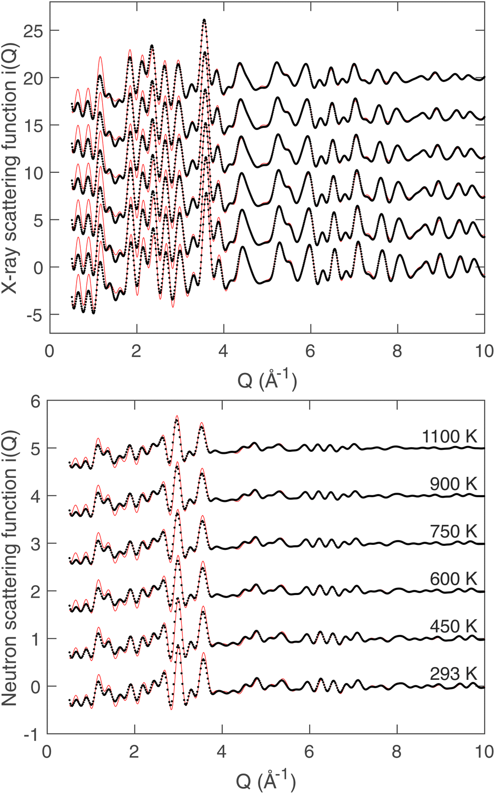Fig. 4 Synchrotron (top) and neutron (bottom) scattering functions i(Q) for LLZO at the studied temperatures. A constant offset has been applied to separate data from different temperatures, with the order in temperature for both plots defined in the plot for neutron scattering. In each case the data are shown as black points, and the results from RMC modelling are represented by the red solid lines.

Fig. 5 Synchrotron (top) and neutron (bottom) pair distribution functions D(r) obtained from Fourier transform of the scattering functions. Experimental data for all temperatures are represented as black points. The red solid lines in the case of the neutron PDF is the result of the calculation by RMC, but in the case of the X-ray PDF where these data were not used in the RMC, the red lines are the functions reconstructed from the partial g_mn(r) functions generated from the RMC configurations with suitable scalings of atomic scattering to match the meaning of the experimental function and normalised. A constant offset has been applied to separate results for different temperatures, and the order of temperatures is the same as that given in Fig. 4.

Fig. 6 Neutron Bragg diffraction data (black points) for LLZO modelled using RMC analysis (red solid lines). Data for different temperatures are shown with a constant offset as in Fig. 4 and 5.

2.7 Molecular dynamics simulations

Classical molecular dynamics (MD) simulations were performed using the package.⁴⁸ Empirical force-fields were used, which include the long-range Coulomb potential and short-range Buckingham potential functions to describe the energy between two ions of type m and n, E_mn(r), assumed to be functions of inter-ionic separation r only:

The ions were treated as rigid entities with no induced polarisation, and assigned formal charges, Q_La = +3e, Q_Zr = +4e, Q_Li = +e, Q_O = −2e, where e is the positive unit charge value. The parameters of the force field were taken from the work of Wang et al.,¹² who used a combination of literature values (for example, the parameters for the O–O interactions were taken from the model for silica of Sanders et al.⁴⁹) and new values; the parameters of the force field are given in Table 1. The starting configurations were the same as used in the RMC work (linear dimensions of around 52 Å, and 12 288 atoms), and simulations were performed at the same temperatures as in the neutron and X-ray total scattering measurements.

Table 1 Force field parameters for the molecular dynamics simulations, from the work of Wang et al.,¹² with interactions between cations assumed to be given only by the Coulomb interaction. Ions are assigned their formal charge values. The parameters are defined by eqn (7)

	A (eV)	ρ (Å)	C (eV Å^6)
Zr–O	1385.02	0.35	0
La–O	4579.23	0.3044	0
Li–O	632.102	0.2906	0
O–O	22764.30	0.1490	27.63

---

Simulations were performed within thermodynamic ensembles that were either constant-stress^50,51 and constant temperature,^52,53 or the standard constant-volume constant-energy microcanonical conditions. Simulations were performed using a time step of 0.001 ps.

3 Results and discussion

3.1 Ionic conductivity

3.1.1 Electrochemical impedance spectroscopy. Fig. 7 shows typical Nyquist plots derived from EIS measurements on LLZO at selected temperatures. Only at room temperature is a part of a semicircle visible at high frequencies, attributable to the grain boundary contribution, followed by a low frequency tail attributable to the build up of charge at the blocking gold electrodes. At all other temperatures the semicircle lay outside the frequency window of the measurements and therefore only total resistances could be measured directly from the interpolated intercept of the tail with the real axis. The total ionic conductivity is found to be about 2.1 × 10⁻⁶ S cm⁻¹ at room temperature, about two orders of magnitude lower than in previous studies,¹¹ possibly reflecting a greater contribution from the grain boundaries to the total resistance measured in the present work. On the other hand, the ionic conductivity is still higher than that of the tetragonal phase.

Fig. 7 Nyquist plots of the AC impedance data for LLZO at a number of temperatures.

The diffusion constant can be calculated from the conductivity using the Nernst–Einstein-equation:

where Q is the charge of the lithium and N is the concentration of lithium ions. The dependence of the extracted values of log  D on 1000/T are given in Fig. 8. Assuming that D follows an Arrhenius behaviour,

D = D₀ exp(−E_a/k_BT), (9)

Fig. 8 Logarithm of diffusion constant D versus 1000/T for both experimental conductivity data at lower temperatures (open circles) and from MD simulation (filled circles). The two lines are fitted to the parts of the data sets (dashed and continuous respectively) consistent with the linear relationship. The two slopes give activation energies of 0.36 eV for the experimental conductivity data and 0.22 eV for the simulation data.

The data at higher temperatures are consistent with activation energy E_a = 0.36 eV. This is very close to the value E_a = 0.34 eV obtained over a narrower range of temperatures by Li et al.¹¹ The prefactor D₀ = 45.0 Ų ps⁻¹.

3.1.2 Lithium-ion diffusion studied by molecular dynamics simulations. The diffusion of lithium ions over time can be obtained from the standard result for the mean-square displacement of the ions, 〈r²〉, over time, t, that is obtained from a general diffusion equation:

〈r²〉 = q_iDt (10)

where q_i is numerical constant that depends on dimensionality and is equal to 6 for 3-dimensional diffusion. The variation of the mean-squared displacements of the Li⁺ ions with time for the different temperatures is shown in Fig. 9. From eqn (10) values for the diffusion constant for different temperatures have been extracted from the data of Fig. 9, and the results are compared with experimental data in Fig. 8. The slope of the data at higher temperatures yields an activation energy of E_a = 0.17 eV. This is about two times lower than for experiment, but a difference is to be expected since the MD results are purely for the bulk whereas the experimental value contains contribution from diffusion along the grain boundaries. The diffusivity pre-factor D₀ in eqn (9) is 1.43 Ų ps⁻¹. This is substantially lower than from experiment, although the lower activation energy means that the diffusivity is higher at lower temperatures, as seen in Fig. 8.

Fig. 9 Dependence of the mean squared displacement of lithium ions for temperatures over the range 293–1100 K calculated by MD simulation.

3.2 Crystal structure analysis

Rietveld refinement of the crystal structure of LLZO from neutron powder diffraction data was performed by describing the crystal structure with sites Li₁ and Li₂ for the lithium ions, with site occupancies constrained to ensure that the total amount of lithium in the two sites was commensurate with the stoichiometric chemical formula. Thus the respective site occupancies c₁ and c₂ were constrained as c₁ + 2c₂ = 7/3. Attempts were made to include the Li₃ site too, but unlike the experience of previous workers, we found that it was hard to produce stable refinements. In any case, the aim was not to characterise the lithium distribution using crystallographic sites, but simply to check that our results were consistent with previous work, although our measurements do extend beyond the range of temperatures in previous studies.

We note that some previous authors attempted to include site occupancies for aluminium,^8,9,11 allowing the value to be refined, and others treated the total lithium content as a refined quantity by not adding constraints on the sum of all site occupancies.^5,9–12 However, the inconsistency of reported results, and indeed our own experience with regard to the stability of refinements, and corresponding estimates of the standard errors, suggests to us that the amount of aluminium and reduction in the total amount of lithium is not significant when compared to the sensitivity of the data to exact chemical composition in the Rietveld refinements. Thus we have used the stoichiometric chemical formula in the Rietveld refinements and in the subsequent RMC studies, whose initial configurations are generated directly from the results of the Rietveld refinement (Section 2.6).

The structural parameters of LLZO obtained from Rietveld refinement of the neutron scattering data for all temperatures are given in Table 2. The values of the atomic fractional coordinates are consistent with previous refinements.^5–13,15,17 As noted earlier, the refined values of site occupancies are not consistent between previous studies. However, our value of c₁ is consistent with that obtained in an earlier neutron powder diffraction study, although in that case a stable refinement that included the Li₃ site was achieved. The refinements suggest that the region around the Li₂/Li₃ sites is nearly fully occupied by one lithium ion, leaving the Li₁ site with occupancy typically of between 1/3–1/2, as suggested by previous refinements.^11,13 The obvious conclusion from this is that diffusion occurs by atoms moving between the Li₂/Li₃ sites via vacant Li₁ sites.

Table 2 Lattice parameters, atomic fractional coordinates and Li₂ site occupancy of Li₇La₃Zr₂O₁₂ obtained from Rietveld refinement. The crystal structure has space group Ia3̄d. Zr has fractional coordinates 0,0,0, La has fractional coordinates 1/4, 0, 1/4, Li₁ has fractional coordinates 3/8, 0, 1/4, defining the usual tetrahedral site in the garnet structure, and Li₂ has fractional coordinates 1/8, y, y + 1/4. Note that the Li₁ site occupancy is constrained from the value of that of the Li₂ site as described in the text. Occupancies for the data at 1100 K were unstable in the refinement and their values were therefore set by hand. Standard deviations are given for the last significant figures in brackets

T (K)	a (Å)	O x	O y	O z	Li2y	Li2 occ.	Li1 occ.
298	12.92244(7)	0.10246(5)	0.19708(5)	0.28088(4)	0.1792(2)	0.987(3)	0.359(6)
450	12.95295(13)	0.10216(6)	0.19682(6)	0.28096(5)	0.1781(3)	0.877(4)	0.579(8)
600	12.98000(7)	0.10224(6)	0.19716(6)	0.28072(5)	0.1797(3)	0.909(12)	0.52(2)
750	13.00941(6)	0.10218(5)	0.19724(5)	0.28082(5)	0.1799(2)	0.942(3)	0.449(6)
900	13.04482(6)	0.10204(5)	0.19765(5)	0.28051(5)	0.1807(3)	0.972(3)	0.389(6)
1100	13.08637(7)	0.10175(6)	0.19752(5)	0.28051(6)	0.1804(3)	1	1/3

---

The lattice parameters reported in Table 2 show a linear thermal expansion. The coefficient of volumetric thermal expansion from the data is α_V = 11.8 × 10⁻⁶ K⁻¹. This is slightly lower than the value inferred from the data of Han et al.¹³

3.3 Local structure analysis

3.3.1 Behaviour of the La₃Zr₂O₁₂ network. Selected partial PDF (pPDF) functions g_mn(r) are shown in Fig. 10, comparing the results from both MD and RMC analyses. The larger differences between the RMC and MD results are for the Li–O pPDF (Fig. 10a), which we will discuss below (Section 3.4). The La–O and Zr–O pPDFs (Fig. 10b and c) show close agreement between the RMC and MD results. In the case of the La–O pPDF (Fig. 10b) the first peak is broader and the second peak narrower in the MD results, compared to the corresponding RMC results. A similar pattern is seen in the Zr–O pPDF (Fig. 10c) but to a lesser extent. The O–O pPDF (Fig. 10d) shows some differences between the RMC and MD results at low r, which may reflect the behaviour around the Li⁺ ions.

Fig. 10 The partial pair distribution functions g(r) calculated from RMC simulations (black curves) and MD simulations (red curves) for (a) Li–O, (b) La–O, (c) Zr–O and (d) O–O atom pairs at low-r, shown for all temperatures as indicated in panel (a). A constant offset has been applied to separate data from different temperatures, with the key to temperature values given in the Li–O function (a).

The distributions of the Zr–O and La–O bond lengths from both RMC and MD simulations at each temperature are shown in more detail in Fig. 11. One very interesting feature from both the RMC and MD results (actually more strongly seen in the latter) is that the distribution of La–O distances is not symmetric but shows a wider spread to larger distances. This suggests quite a strong anharmonicity, and reflects a similar situation seen in CsPbI₃ (ref. 54), albeit to a lesser extent. In the crystal structure there are two distinct La–O bond lengths (2.53 and 2.63 Å at a temperature of 1100 K), but these are not sufficiently different to explain the width of the distribution.

Fig. 11 The distributions of La–O and Zr–O bond lengths (top and bottom respectively) at the different temperatures (blue to red corresponds to 293 K to 1100 K) in both the RMC and MD models (left and right respectively), each averaged over six independent configurations.

The distributions of O–Zr–O and O–La–O bond angles from both RMC and MD analyses at the different temperatures are shown in Fig. 12. The RMC and MD results are consistent in most respects. The key features in the O–Zr–O distribution reflect a slightly distorted octahedron, with nearly right-angle bond angles deviating from the ideal 90° by a few degrees. The fluctuations in the O–Zr–O bond angles are slightly larger in the RMC than in the MD, and there are features to indicate a few large distortions of around 20°.

Fig. 12 The distributions of O–La–O and O–Zr–O bond angles (top and bottom respectively) at the different temperatures (blue to red corresponds to 293 K to 1100 K) in both the RMC and MD models (left and right respectively), each averaged over six independent configurations.

The LaO₈ polyhedron is not of regular shape. There are two distinct La–O distances in the average structure as noted above, and of the 28 O–La–O bond angles there are 10 distinct angle values. Thus this distribution of O–La–O angles is rather more complicated than for the angles within the ZrO₆ octahedra, as seen in Fig. 12. The MD and RMC results both capture this distribution, with the peaks in the distribution from the RMC simulation being slightly broader than from the MD simulation. There is again evidence for some unreasonably low angles in the RMC simulation, with the small peak around 50–60°.

The data for bond lengths and angles (Fig. 11 and 12 respectively) show that the ZrO₆ and LaO₈ polyhedra retain their integrity across the full range of temperatures in both RMC and MD calculations (aside from some low angles in the RMC simulation), with only a slight broadening with increasing temperature. Thus we conclude that the backbone network structure with channels for Li-ion diffusion remains robust across the studied temperature range.

3.4 Distribution of lithium ions

3.4.1 Visual representations of the lithium-ion density. By collapsing the configurations, each of which contains 64 unit cells, down into a single unit cell, then combining the atoms of 6 configurations at a time, and drawing only the lithium ions, we can get a feel for the diffusion pathways. Examples from both RMC and MD calculations (at 273 K) are shown in Fig. 13. The two simulations are consistent with each other, particularly with regards to the fact that the Li₁ sites appear to be connected via pathways passing through the Li₂ sites. One key difference in these plots is that the distribution of atomic positions in the RMC configurations appears to be broader than in the MD configurations. Thus the spatial distribution of the network of lithium positions is perhaps more easily seen in the distribution from the MD configurations.

Fig. 13 Distribution of the instantaneous positions of the lithium ions in the RMC (left) and MD (right) configurations, at temperatures of 293 K (top) and 1100 K (bottom). These images were obtained by collapsing each configuration down to one unit cell and then adding the atoms from 6 separate configurations. The network of lithium positions is more easily seen in the results from the MD configurations, but the same network characterises the distributions of the RMC configurations. The positions of one set of Li₁ and Li₂ sites are indicated in the plot of the MD results at 293 K (top right). These images were produced using CrystalMaker®.²¹

Simply plotting atoms in a three-dimensional space is a poor way to represent the quantitative density of atoms. Such a plot, in which points are represented by finite-size spheres, tends to exaggerate the visual representation of the lower-density regions and masks the true density of the higher-density regions which contain many overlapping spheres. In Fig. 14 we represent the densities of lithium ions in the collapsed configurations as isosurfaces, and show results for the lowest and highest temperatures for both the RMC and MD configurations. The density plots show concentrations of atoms around the Li₁ and Li₂ centres (the latter encompass the Li₃ sites), and highlight the pathways connecting Li₁ sites via the Li₂/Li₃ centres. In Fig. 1 we show the relationship between the network of lithium positions and the rest of the crystal structure by plotting one of the lithium atom density isosurfaces together with the crystal structure represented as connected ZrO₆ and LaO₈ polyhedra.

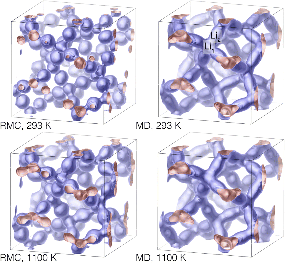Fig. 14 Density isosurfaces of lithium positions in the RMC (left) and MD (right) configurations at 293 K (top) and 1100 K (bottom). The positions of one set of Li₁ and Li₂ sites are indicated in the plot of the MD results at 293 K (top right), as in Fig. 13. These images were produced using CrystalMaker®.²¹

The shapes of the density isosurfaces show little differences between the range of temperatures, except that there is a bulging of the necks connecting the Li₁ and Li₂ centres. This point is pertinent for the subsequent analysis: it appears that even at high temperatures the lithium ions are mostly located around the Li₁ and Li₂/Li₃ centres.

Isosurface representations highlight the network containing the distribution of positions of lithium atoms as a visual representation, but are limited for more quantitative analysis. Because the Li₁–Li₂ pathway does not lie in a simple crystallographic plane, projections of atomic density (integrating the density in the perpendicular direction) are more useful than slices taken through the three-dimensional crystal. Fig. 15 shows the projections of the lithium-ion densities onto a surface perpendicular to the crystallographic 4₁ axis. To reduce statistical noise, not only did we combine six independent configurations in each case but we also applied some of the symmetry operations. In the case of LLZO, the use of projections is helped by the fact that there is limited overlap of the Li₁ positions and no overlap of the Li₂ positions, as seen in Fig. 1.

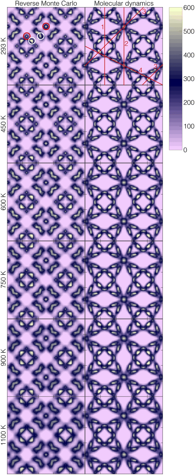Fig. 15 Lithium-ion densities of LLZO, shown in projection down the [001] axis, from RMC (left) and MD (right) configurations for each of 6 temperatures. Each square plot shows a single unit cell. The right-hand side shows the colour scheme to indicate the density, with pink representing zero density and yellow showing the maximum density. In the top left panel the red circles highlight examples the tetrahedral Li₁ sites, and the white circles highlight examples of the Li₂ sites. The red lines in the top right panel indicate four lines used in further analysis in Fig. 16.

Representations of the lithium-ion density are shown in Fig. 15 for both the RMC and MD configurations, for all temperatures. The colour contour maps are shown in projection down [001], and show a single unit cell in each case. The density plots show clearly the accumulation of atomic density around the Li₁ and Li₂ positions, as indicated in the top RMC image of Fig. 15. There are three points to make. The first is that the RMC and MD configurations look different at first sight, but we will see that is because of the visual impact of the differences in the distributions around Li₂/Li₃ centres and differences in the lithium atomic density within the channels connecting lithium sites, rather than because of differences in the major part of the distributions. We will explore the differences quantitatively below. The second point is that both the RMC and MD configurations display a large concentration of the density of lithium ions around the Li₁ and Li₂/Li₃ centres, which are identified by the red (Li₁) and white (Li₂) circles in one of the images in Fig. 15. The third point is that the visual impression of changes with temperature are only slight. At the highest temperatures most of the lithium ions appear to still be associated with the Li₁ and Li₂ centres. However, some increased density between the centres following the lines of the network can be seen, and this will be demonstrated more quantitatively next.

3.4.2 Quantitative analysis of the lithium-ion density. To quantify the analysis of the lithium-ion density, we show in Fig. 16 the density along four lines in the projections that contain the Li₁ and Li₂ centres. These are illustrated by the red lines in the image for the density projection for the MD results at 293 K in Fig. 15. We consider each of these lines in turn.

Fig. 16 Lithium ion density profiles for thin slabs through the projections shown in Fig. 15 calculated from configurations generated by RMC (left) and MD (right). From top to bottom are the slices indicated as lines 1 to 4 in the top-right panel of Fig. 15. Temperatures from 293–1100 K are indicated by the colour change from blue to red. The range of x spans the full repeat distance across the unit cell.

Line 1: this line, parallel to the [100] axis, passes through four Li₁ centres at starting position x = 1/8 and separated by Δx = 1/4. These peaks can be clearly seen in both the results from the RMC and MD configurations. The distributions are slightly broader in the RMC configurations.

The effect of temperature appears to show some broadening of the peaks, but the clearer effect is the decrease in the heights of the peaks.

Line 2: this line is parallel to Line 1, but is displaced by a/4 and passes through two Li₁ centres at positions x = 1/4 and x = 3/4, having a different orientation of the environment around the individual Li₁ centres (recall that the 4 nearest Li₁ sites to any other Li₁ site form a distorted, not regular, tetrahedral arrangement). Results from both the RMC and MD configurations show the two peaks associated with the two Li₁ centres. For the MD configurations the peaks are slightly broader than for Line 1, reflecting the different orientation of the Li₁ centres. It can be seen from Fig. 15 that the Li₁ site appears to have something of a pancake shape. The major difference between the RMC and MD results is that this line passes through areas of higher lithium-ion density around the Li₂/Li₃ centres in the RMC model that are not present in the MD configurations, reflecting some differences in the distributions around these centres.

The effect of temperature is the same as for Line 1. In the case of the MD results the peak is simply broadened, but in the case of the RMC results it can be seen that the reduction in the heights of the peaks is offset by the increase in heights of the peaks of the site bands coming from the overlap of the line with the density associated with the Li₂/Li₃ centres.

Line 3: this line is parallel to [110] and passes through Li₁ centres in both orientations (crossing both Line 1 and Line 2), and passes near the Li₂ sites. The origins of the line are in an area of the projection with low density of lithium ions within a square defined by four Li₁ sites. The line passes through one set of Li₁ centres at positions x = 1/4, 3/4. It passes through a set of Li₂ centres at x ≃ 1/16, 7/16, 9/16 and 15/16. Between the Li₁ and Li₂ centres the line passes close to pairs of Li₂ sites. For both the RMC and MD data the peaks associated with the two Li₁ sites and four Li₂ centres can clearly be seen in Fig. 16. The main difference between the RMC and MD results lies in the density profiles either side of the two Li₁ peaks, which reflect the slightly different shapes of the broad distributions associated with the Li₂/Li₃ centres.

The effect of temperature is a decrease in the heights of the peaks as before. In the case of the MD configurations there is an increase in the peaks associated with the distribution either side of the Li₁ peaks at x = 1/4, 3/4 associated with the line passing near (not through) the nearby Li₂/Li₃ centres.

Line 4: this line is parallel to [120] and passes through the Li₁ centres in both orientations as well as passing through the Li₂ centres. The origins are within the flattened lozenges defined by four Li₁ centres. One Li₁ centre is at position x = 1/2, and the other two in the alternative orientation are at x = 1/4, 3/4. The Li₂/Li₃ centres that are intersected by Line 4 are positioned between two Li₁ centres either side of x = 1/2, and the line also passes by the Li₂/Li₃ centres that lie the other side of the two Li₁ centres of the alternative orientation. All of these features are seen in the density profiles in Fig. 16. The main difference between the RMC and MD data concerns the height of the Li₁ peak at x = 1/2, which is the same as the difference in Line 2.

Regarding the variation with temperature, the comments made with regard to Line 3 apply to Line 4 also.

The key similarities in the distributions of the lithium ions in the RMC and MD configurations as revealed by this analysis is that in both cases the lithium ions are mostly clustered around the Li₁ and Li₂/Li₃ centres. The key differences are in the details of the shape of the distribution around the Li₁ sites, where the distribution is more anisotropic in shape in the MD configurations than in the RMC configurations, and in the shape of the distribution around the Li₂/Li₃ centres, which is not constrained by symmetry.

To quantify the differences between the RMC and MD simulations with regard to the distribution of the lithium ions around the Li₁ and Li₂/Li₃ centres, and the way these change with temperature, we analysed the number of lithium ions in the vicinities of the Li₁ site and the nominal Li₂ sites, the latter being located (for this analysis) half way between closest Li₁ sites. There is a small separation (around 0.1 Å) between this ideal position and the position refined from the powder diffraction data¹¹ (see also Table 2). The results are shown in Fig. 17. For this analysis we simply counted the number of lithium ions lying within a certain radius of each Li₁ and Li₂ site. Fig. 17 shows the normalised number density for a range of distances from the two sites. We might have converted this to a distribution function by dividing by the square of the distance, which would give a peak at zero distance rather than zero value, but in practice we found that this over-emphasises the statistical noise.

Fig. 17 Lithium ion density distributions around the Li₁ and Li₂ sites (top and bottom respectively) as functions of distance from the nominal site positions, calculated from configurations generated by the RMC (left) and MD (right) methods. Temperatures from 293–1100 K are indicated by the colour change from blue to red.

The data of Fig. 17 for the Li₁ site show significant differences between the results from RMC and MD results in terms of the spread of distances. The key point is that the distribution is broader for the MD configurations, reflecting the pancake distribution discussed earlier, and the distribution then merges into that for the distant Li₂ site. In both cases the distribution around the Li₁ sites broadens and the lithium cations move into the channels connecting the Li₁ and Li₂/Li₃ sites.

In contrast, the distributions around the nominal Li₂ sites are around 50% broader than around the Li₁ sites in both cases, and are similar in both the RMC and MD configurations in this view of the lithium ion density, even though the actual distributions, as seen in the density plots of Fig. 15, are different in shape. The distributions around the nominal Li₂ sites broaden slightly on increasing temperature, and although there is an increase in the density of lithium ions with temperature at larger distances there is less of a decrease in the density near the Li₂ sites.

In Fig. 18 we show the change in lithium-ion density with temperature. These data have been calculated from the data in Fig. 17 by averaging around a small region at distances of 0.8 Å and 1.2 Å for the Li₁ and Li₂ sites, respectively. For both sites in both the RMC and MD configurations we see the growth in the density between Li₁ and Li₂/Li₃ sites with temperature, but there are differences between the two models. In the RMC results we see growth in density in the channels near the Li₁ and Li₂/Li₃ sites, but in the MD results we see much larger density in the channels near the Li₁ site than in the RMC results. The data in both plots in Fig. 18 cannot reasonably be described by a simple Arrhenius-like behaviour.

Fig. 18 Variation of the density of lithium ions around distances 0.8 Å and 1.2 Å from sites Li₁ and Li₂, respectively, with temperature, calculated from the configurations generated by the RMC (left) and MD (right) methods.

This detailed analysis has shown three things. Firstly, in both RMC and MD models, most of the lithium ions have positions around the Li₁ and Li₂/Li₃ centres, with only a small amount of lithium within the network of channels connecting lithium sites. Secondly, there are differences in the shapes of the distributions of the lithium ions around these two sites in the RMC and MD models. We recall that the Li₁ site is one of special symmetry (4̄), whereas the Li₂ has no special symmetry and thus the shape of the ionic distribution is not constrained by symmetry. Thirdly, we can see that the effect of temperature is to allow some of the lithium ions to leave the regions of higher density around the Li₁ and Li₂/Li₃ centres and move into the network of channels connecting the lithium sites.

The main conclusion, when considering the information common to both the RMC and MD modelling, is that the lithium ions in LLZO are mostly located around the Li₁ or Li₂/Li₃ centres, with some motion between centres enabled by thermal excitation. In the next part, where we consider the dynamics calculated by the MD simulations, we will see more evidence for the localisation of the lithium ions.

3.5 Ionic vibrational density of states

From the MD simulations we calculated the velocity autocorrelation functions (VACFs) as functions of time, t, from the set of velocities v_m(t) for each atom type m:where the angled brackets denote averaging over a range of starting times in the simulation, and over all atoms of the same type. The VACFs for each atom type were calculated for 6 different simulations and averaged, and are shown in Fig. 19. It can be seen that there is little variation with temperature in each case.

Fig. 19 The velocity autocorrelation functions (VACF) for Li, La, Zr and O atoms for all temperatures calculated from the molecular dynamics simulations. Temperatures from 293–1100 K are indicated by the colour change from blue to red.

Fourier transformation of the VACFs gives the power spectra Z_m(f) for a range of frequencies f. The mass-weighted combination of the individual Z_m(f) spectra gives the full phonon density of states. Fig. 20 shows the power spectra for the four types of atom, which we consider in turn below.

Fig. 20 The power spectra of Li, La, Zr and O atoms for all temperatures obtained by Fourier transformation of the VACFs shown in Fig. 19. Temperatures from 293–1100 K are indicated by the colour change from blue to red.

The lanthanum Z(f) shows a strong peak at low frequencies centred on 5 THz. This lower frequency, as compared with the other atom types, reflects the fact that La has the largest mass. The zirconium Z(f) shows a wider spread of frequencies, the higher of which will be associated with Zr–O bond stretching modes. The Z(f) includes the same peak at 5 THz seen for La, a large peak at 7 THz, and other features at higher frequencies. We note a peak seen at 13 THz. The oxygen Z(f) reflects the interaction of this anion with all three different cations, and has a broad spectrum across the frequency range from 0–32 THz. The shape of the spectrum has features reflecting the peaks in the zirconium Z(f), including the peak at 13 THz, but also has features seen in the lithium Z(f), which we now discuss.

Lithium is the lightest element in the system and so, if bonded to the wider network, will display features at higher frequencies than La or Zr, which is indeed seen to be the case. The Li Z(f) shows features seen in the power spectra of other elements, such as the peaks at 5 THz (La); it has a peak at 12 THz which is slightly lower than the peaks at 13 THz seen in Z_Zr(f) and Z_O(f), but these distributions contain many more frequencies than in single peaks so the difference is not significant. It can be concluded that over most of the frequency range the lithium ion appears to be vibrating as a bound particle, with the higher frequency reflecting the light mass of the atom compared with the other atoms. The coincidence of the upper frequencies in the power spectrum of lithium with that of oxygen suggests that the bound Li–O pair execute bond-stretching types of vibration.

The lithium power spectrum, Z_Li(f), shown in Fig. 20 also has an interesting feature at low frequencies. For an ideal solid, it is found that Z(f) ∝ f² at low frequencies, reflecting the contribution of the acoustic modes (the famous Debye function). Finding this behaviour exactly is difficult in a simulation because the Z(f → 0) part of the power spectrum is the part most susceptible to noise in C(t), and any noise might break the equality ∫C(t)dt = 0 that is implicit in the expectation that Z(f = 0) = 0. Nevertheless, we see in the Z(f) spectrum for lithium a non-zero intercept at f = 0 that increases on heating. This is to be expected if some of the motions of the lithium atoms are diffusion rather than vibration, with an increase in the value of Z_Li(f = 0) on heating as more ions are excited into diffusion motions. Thus we can infer from the results for Z_Li(f) shown in Fig. 20 that the dynamics of the lithium ion reflect some degree of diffusion motion in addition to vibrational motion. However, the contribution is small, and the main conclusion from the Z_Li(f) data is that lithium ions are primarily bound to the sites identified in the structural analysis of the diffraction and total scattering experimental studies and MD simulations, executing vibrational motions, with only a small fraction of the motions corresponding to diffusion.

4 Conclusions

In this paper we have explored the three-dimensional distribution of lithium ions in the fast-ion conductor Li₇La₃Zr₂O₁₂ using a combination of simulation methods, namely the RMC method based on both neutron and X-ray total scattering data, and the MD method. There is a high degree of consistency between the two methods, albeit with some differences concerning the distribution of lithium positions around the Li₂/Li₃ centres. The backbone La₃Zr₂O₁₂ network is robust at all temperatures. The network defines a set of curved pathways for the motions of lithium ions.

The results of the MD simulations are consistent with the measurements of ionic conductivity measurements presented in Section 3.1. Differences between results are likely to reflect inaccuracies in the interatomic potential and are not significant.

The key picture to emerge from this study is that in LLZO only a small fraction of the lithium ions are mobile at any instant in time. Instead most of the lithium ions are found around either the Li₁ or Li₂ centres, bonded to oxygen atoms at these sites, and participating in the higher frequency vibrations. The Li₂ sites are nearly fully occupied, whereas the Li₁ sites typically have around 2/3 vacancies. Thus lithium-ion diffusion mostly occurs by the ions moving between the large Li₂ sites via empty Li₁ sites.

Author contributions

Haolai Tian: investigation, formal analysis, funding, validation, software, writing (original draft), writing (review & editing), visualisation. Guanqun Cai: investigation, formal analysis, writing (review & editing). Lei Tan: investigation, writing (review & editing). He Lin: investigation, writing (review & editing). Anthony E. Phillips: writing (review & editing). Isaac Abrahams: writing (review & editing). David A. Keen: investigation, formal analysis, writing (review & editing). Dean Keeble: investigation, formal analysis, writing (review & editing). Andy Fiedler: investigation, writing (review & editing). Junrong Zhang: writing (review & editing). Xiang Yang Kong: conceptualization, funding acquisition, supervision, writing (review & editing). Martin T. Dove: funding acquisition, investigation, formal analysis, methodology, validation, supervision, software, writing (original draft), writing (review & editing), visualisation.

Conflicts of interest

There are no conflicts to declare.

Acknowledgements

Haolai Tian is grateful to the China Scholarship Council (No. 201704910231) for financial support. Guanqun Cai and Lei Tan were supported by student scholarships also from the China Scholarship Council. This work is also funded by the National Natural Science Foundation of China (Grant Numbers 11675195 (MTD and LT) and 21761132004 (XYK and AF)). This research used radiation facilities operated by ISIS and Diamond of STFC for provision of beam time (project numbers RB1910237 and ee19378 respectively). The archived neutron scattering data are available with DOI: 10.5286/ISIS.E.RB1910237. The research also made us of the HPC facility of China Spallation Neutron Source, supported by IHEP Computer Center, and Yakang Li in particular. We are grateful to David Palmer of CrystalMaker Software Limited for support in using CrystalMaker®,²¹ particular for the iso-density surface plots shown in Fig. 1 and 14.

References

1. R. Murugan, V. Thangadurai and W. Weppner, Angew. Chem., Int. Ed., 2007, 46, 7778–7781.
2. A. J. Samson, K. Hofstetter, S. Bag and V. Thangadurai, Energy Environ. Sci., 2019, 12, 2957–2975.
3. K. Kataoka, J. Ceram. Soc. Jpn., 2020, 128, 7–18.
4. C. Wang, K. Fu, S. P. Kammampata, D. W. McOwen, A. J. Samson, L. Zhang, G. T. Hitz, A. M. Nolan, E. D. Wachsman, Y. Mo, V. Thangadurai and L. Hu, Chem. Rev., 2020, 120, 4257–4300.
5. C. A. Geiger, E. Alekseev, B. Lazic, M. Fisch, T. Armbruster, R. Langner, M. Fechtelkord, N. Kim, T. Pettke and W. Weppner, Inorg. Chem., 2011, 50, 1089–1097.
6. J. Awaka, A. Takashima, K. Kataoka, N. Kijima, Y. Idemoto and J. Akimoto, Chem. Lett., 2011, 40, 60–62.
7. K. Kataoka and J. Akimoto, J. Ceram. Soc. Jpn., 2019, 127, 521–526.
8. D. Rettenwander, G. Redhammer, F. Preishuber-Pflügl, L. Cheng, L. Miara, R. Wagner, A. Welzl, E. Suard, M. M. Doeff, M. Wilkening, J. Fleig and G. Amthauer, Chem. Mater., 2016, 28, 2384–2392.
9. H. Buschmann, J. Dölle, S. Berendts, A. Kuhn, P. Bottke, M. Wilkening, P. Heitjans, A. Senyshyn, H. Ehrenberg, A. Lotnyk, V. Duppel, L. Kienle and J. Janek, Phys. Chem. Chem. Phys., 2011, 13, 19378–19392.
10. H. Xie, J. A. Alonso, Y. Li, M. T. Fernández-Díaz and J. B. Goodenough, Chem. Mater., 2011, 23, 3587–3589.
11. Y. Li, J.-T. Han, C.-A. Wang, S. C. Vogel, H. Xie, M. Xu and J. B. Goodenough, J. Power Sources, 2012, 209, 278–281.
12. Y. Wang, A. Huq and W. Lai, Solid State Ionics, 2014, 255, 39–49.
13. J. Han, J. Zhu, Y. Li, X. Yu, S. Wang, G. Wu, H. Xie, S. C. Vogel, F. Izumi, K. Momma, Y. Kawamura, Y. Huang, J. B. Goodenough and Y. Zhao, Chem. Commun., 2012, 48, 9840–9842.
14. J. Percival, E. Kendrick, R. I. Smith and P. R. Slater, Dalton Trans., 2009, 5177–5181.
15. J. Awaka, N. Kijima, H. Hayakawa and J. Akimoto, J. Solid State Chem., 2009, 182, 2046–2052.
16. J. Awaka, N. Kijima, K. Kataoka, H. Hayakawa, K. ichi Ohshima and J. Akimoto, J. Solid State Chem., 2010, 183, 180–185.
17. R. Wagner, G. J. Redhammer, D. Rettenwander, A. Senyshyn, W. Schmidt, M. Wilkening and G. Amthauer, Chem. Mater., 2016, 28, 1861–1871.
18. M. P. Stockham, A. Griffiths, B. Dong and P. R. Slater, Chem. –Eur. J., 2022, 28, e202103442.
19. M. Klenk and W. Lai, Phys. Chem. Chem. Phys., 2015, 17, 8758–8768.
20. G. Larraz, A. Orera, J. Sanz, I. Sobrados, V. Diez-Gómez and M. L. Sanjuán, J. Mater. Chem. A, 2015, 3, 5683–5691.
21. D. C. Palmer, Z. Kristallogr. – Cryst. Mater., 2015, 230, 559–572.
22. V. F. Sears, Neutron News, 1992, 3, 26–37.
23. R. L. McGreevy and L. Pusztai, Mol. Simul., 1988, 1, 359–367.
24. M. T. Dove, M. G. Tucker and D. A. Keen, Eur. J. Mineral., 2002, 14, 331–348.
25. D. A. Keen, M. G. Tucker and M. T. Dove, J. Phys.: Condens. Matter, 2005, 17, S15–S22.
26. M. T. Dove and G. Li, Nucl. Anal., 2022, 1, 100037.
27. A. C. Hannon, Nucl. Instrum. Methods Phys. Res., Sect. A, 2005, 551, 88–107.
28. A. K. Soper, GudrunN and GudrunX : Programs for Correcting Raw Neutron and X-Ray Diffraction Data to Differential Scattering Cross Section, Rutherford Appleton Laboratory Technical Report RAL-TR-2011-013, 2011.
29. O. Arnold, J. C. Bilheux, J. M. Borreguero, A. Buts, S. I. Campbell, L. Chapon, M. Doucet, N. Draper, R. F. Leal, M. A. Gigg, V. E. Lynch, A. Markvardsen, D. J. Mikkelson, R. L. Mikkelson, R. Miller, K. Palmen, P. Parker, G. Passos, T. G. Perring, P. F. Peterson, S. Ren, M. A. Reuter, A. T. Savici, J. W. Taylor, R. J. Taylor, R. Tolchenov, W. Zhou and J. Zikovsky, Nucl. Instrum. Methods Phys. Res., Sect. A, 2014, 764, 156–166.
30. A. C. Larson and R. B. Von Dreele, General Structure Analysis System (GSAS), Los Alamos National Laboratory Technical Report LAUR 86-748, 2004.
31. B. H. Toby, J. Appl. Crystallogr., 2001, 34, 210–213.
32. M. Basham, J. Filik, M. T. Wharmby, P. C. Y. Chang, B. El Kassaby, M. Gerring, J. Aishima, K. Levik, B. C. A. Pulford, I. Sikharulidze, D. Sneddon, M. Webber, S. S. Dhesi, F. Maccherozzi, O. Svensson, S. Brockhauser, G. Naray and A. W. Ashton, J. Synchrotron Radiat., 2015, 22, 853–858.
33. A. K. Soper and E. R. Barney, J. Appl. Crystallogr., 2011, 44, 714–726.
34. D. A. Keen, J. Appl. Crystallogr., 2001, 34, 172–177.
35. D. A. Keen, Crystallogr. Rev., 2020, 26, 141–199.
36. E. Lorch, J. Phys. C: Solid State Phys., 1969, 2, 229–237.
37. E. Lorch, J. Phys. C: Solid State Phys., 1970, 3, 1314–1322.
38. A. K. Soper and E. R. Barney, J. Appl. Crystallogr., 2012, 45, 1314–1317.
39. S. Adams and J. Swenson, Phys. Rev. Lett., 2000, 84, 4144–4147.
40. J. Swenson and S. Adams, Phys. Rev. B: Condens. Matter Mater. Phys., 2001, 64, 024204.
41. S. Adams, Solid State Ionics, 2002, 154–155, 151–159.
42. S. Adams and J. Swenson, J. Phys.: Condens. Matter, 2005, 17, S87–S101.
43. M. G. Tucker, D. A. Keen, M. T. Dove, A. L. Goodwin and Q. Hui, J. Phys.: Condens. Matter, 2007, 19, 335218.
44. M. T. Dove and G. Rigg, J. Phys.: Condens. Matter, 2013, 25, 454222.
45. V. M. Nield, D. A. Keen, W. Hayes and R. L. McGreevy, J. Phys.: Condens. Matter, 1992, 4, 6703–6714.
46. R. L. McGreevy, J. Phys.: Condens. Matter, 2001, 13, R877–R913.
47. D. A. Keen, D. S. Keeble and T. D. Bennett, Phys. Chem. Miner., 2018, 45, 333–342.
48. I. T. Todorov, W. Smith, K. Trachenko and M. T. Dove, J. Mater. Chem., 2006, 16, 1911–1918.
49. M. J. Sanders, M. Leslie and C. R. A. Catlow, J. Chem. Soc. Chem. Commun., 1984, 1271–1273.
50. M. Parrinello and A. Rahman, Phys. Rev. Lett., 1980, 45, 1196–1199.
51. S. Melchionna, G. Ciccotti and B. Lee Holian, Mol. Phys., 2006, 78, 533–544.
52. S. Nosé, Mol. Phys., 1984, 52, 255–268.
53. W. G. Hoover, Phys. Rev. A, 1985, 31, 1695–1697.
54. J. Liu, A. E. Phillips, D. A. Keen and M. T. Dove, J. Phys. Chem. C, 2019, 123, 14934–14940.

---