In situ investigation of ion exchange membranes reveals that ion transfer in hybrid liquid/gas electrolyzers is mediated by diffusion, not electromigration

Abstract

Ion-exchange membranes (IEMs) play a crucial role in (photo)electrochemical conversion and storage devices such as (photo)electrolyzers, electrodialysis cells, fuel cells, and batteries. These devices require media separation and selective mass transfer to sustain targeted electrochemical processes. To optimize IEM properties, a thorough understanding of the molecular-level processes under operating conditions is essential. This is particularly important for ion transfer and rejection across polymer membranes. Currently, it is widely accepted that ion transfer occurs through diffusion across the membrane mediated by the local electric field generated by the ionized functional groups and via electromigration induced by the presence of an applied bias between two electrodes placed on each side of the membrane. However, a direct investigation of such processes under working conditions using a chemically-sensitive technique is still missing. In this study, commercially available cation- and anion-exchange membranes were investigated in hybrid liquid/gas electrolyzers by coupling in situ ambient pressure hard X-ray photoelectron spectroscopy (AP-HAXPES) with finite element analysis (FEA). Our findings show that selective ion transport across the membrane separating the liquid from the gas side is driven by diffusion mediated by the ionized functional groups present in the membranes, rather than electromigration. Additionally, we were able to directly detect unwanted polarization fields at the interface between the liquid electrolyte and the polymer membrane. This occurred when the polarity of the applied potential was the same as the charge of the ionized functional groups present in the IEMs. The generation of such polarization fields was attributed to the accumulation of co-ions at the liquid electrolyte/membrane interface, resulting from their rejection and consequent inability to diffuse through the membrane. This leads to a loss in the cell voltage, with detrimental effects on the overall performance and reaction selectivity of hybrid liquid/gas (photo)electrolyzers. This study serves as a proof-of-concept for the use of in situ AP-HAXPES to investigate polymer membranes during operation and sheds new light on the ionic dynamics within the IEMs employed in hybrid liquid/gas electrolyzers.

---

Marco Favaro

Marco Favaro is the deputy head of the Institute for Solar Fuels at the Helmholtz Zentrum Berlin (HZB), Germany. After his PhD in Materials Science and Engineering at the University of Padua (Italy), concluded in 2014, he spent two years as a Post-doctoral fellow at the Joint Center for Artificial Photosynthesis in Berkeley, USA, in the group of Dr Junko Yano. He moved to Germany in 2017 to join the HZB. Here, his research activity focuses on understanding chemical composition/electronic-structural properties/performance interplay in photoelectrocatalysts by coupling operando multimodal spectroelectrochemical investigations with advanced synchrotron-based in situ/operando spectroscopies.

---

1. Introduction

Ion-exchange membranes (IEMs) are critical components of (photo)electrochemical conversion and storage devices such as (photo)electrolyzers, electrodialysis cells, fuel cells, and batteries.^1–4 These devices rely on efficient product and media separation and selective mass transport to sustain targeted electrochemical processes.^5–8 IEMs spatially separate two electrodes into two compartments with their respective electrolytes, where one or more electrochemical reactions takes place. Based on the IEM type and selectivity, specific mobile ions can pass from one compartment to the other, thereby closing the electrical circuit. Once transferred across the membrane, these ions can then further participate in the ongoing electrochemical process(es).⁹ Cation-exchange membranes (CEMs) contain negatively-charged functional groups that promote the transfer of cations (e.g. protons) while preventing the transfer of anions. Anion-exchange membranes (AEMs) instead contain positively-charged functional groups that enable anion transfer (typically hydroxide ions) while rejecting cations. Counter-ions are the mobile ions in the membrane having the opposite charge of the membrane functional groups, whereas co-ions have the same charge.

The optimization of ion selectivity, as well as other key properties such as conductivity and mechanical/chemical stability against degradation, are critical challenges in developing efficient and durable ion-exchange membranes (IEMs) for (photo)electrochemical devices.^10,11 Limitations in these properties can negatively impact the device performance and lifetime.^12–14 While it is generally accepted that ion transfer occurs through diffusion across the membrane mediated by local electric fields generated by ionized functional groups, and via electromigration induced by an applied bias between two electrodes on either side of the membrane,¹⁵ direct investigation of these processes under working conditions using chemically sensitive techniques is still lacking. In this context, X-ray photoelectron spectroscopy (XPS) has been used to characterize IEMs.^16,17 Although these studies provide valuable information about the membrane near-surface chemical composition, the ultra-high vacuum (UHV) conditions in which they are usually carried out do not necessarily reflect the membrane chemical composition and its evolution under relevant operating conditions. Indeed, properties such as mechanical/chemical stability¹⁸ and ionic conductivity^19–21 are closely linked to the hydration level and chemical environment in which the membranes operate.²² Recently, different types of polymer membranes were investigated at near-ambient conditions using different spectroscopy methods,^23,24 including ambient pressure hard X-ray photoelectron spectroscopy (AP-HAXPES).^25,26 AP-HAXPES has proven to be a powerful investigation tool for many energy-related applications.^27–32 When applied to the investigation of IEMs, its distinctive features can provide direct information about the physical/chemical properties of polymer membranes under realistic working conditions:

- AP-HAXPES is a chemically sensitive technique that allows the IEMs' chemical composition of the surface and near-surface region to be retrieved. AP-HAXPES (and, in general, photoelectron spectroscopy) provides additional information on the chemical and oxidation state of the elements present in the IEMs;

- AP-HAXPES can be used to perform spectroscopy on the valence orbitals of the elements present on the IEMs, thereby providing information about the chemical bonding in the material and corresponding density of states;

- AP-HAXPES allows obtaining the information mentioned above while maintaining the electrical polarization on the sample under investigation.^27–29,31 AP-HAXPES enables the direct determination of local built-in electrical potentials by measuring the kinetic energy shift of the detected photoelectrons over a reference state;^27,28,31

- Owing to the relatively high photon energy used, and therefore photoelectron kinetic energy, AP-HAXPES allows obtaining the aforementioned information at relatively high pressure, eventually matching the vapor pressure of water at r. t. (this is also an advantage over the use of soft X-ray photoemission, where operational pressures are limited to a few mbar due to the increased elastic and inelastic scattering of photoemitted electrons at gas molecules);

- AP-HAXPES is a surface sensitive technique, enabling the investigation of the surface and near-surface chemical composition of IEMs from the topmost layer down to about 20–30 nm, making it a suitable technique to study complex interfaces such as triple phase boundaries.

To monitor the near-surface chemical properties of commercially-available cation- and anion-IEMs under realistic conditions, we used synchrotron-based AP-HAXPES. The measurements were carried out at vapor pressures of 15–20 mbar, close to the water vapor pressure at room temperature (relative humidity, RH ∼60–80%). Moreover, we investigated the evolution of the membrane near-surface chemical composition under operating conditions by performing in situ AP-HAXPES while applying electrical potentials of different polarity across the membrane. The membrane was placed in a customized hybrid liquid/gas electrolyzer where half-cell electrochemical reactions occur at the triple phase boundary formed at the solid/liquid/gas interface. These investigations are relevant for the development and optimization of this type of electrolyzer, in particular catholyte-free (zero-gap) devices, which are promising for efficient electrochemical CO₂ reduction.⁹ The substitution of the liquid catholyte with a hydrated gaseous phase circumvents the limited CO₂ solubility in aqueous electrolytes and the dilution of the reaction products, which requires subsequent separation steps for product recovery.^33–35

Consequently, production costs and overall device complexity could be reduced, hence facilitating the scalability of such technology.^33,36 We investigated two ion exchange membranes, Nafion® 115 as a CEM and Fumasep® FAA-3-PK-75 as an AEM. These membranes are used in various (photo)electrochemical devices operating in acidic/neutral and base aqueous environments, respectively.^37–42 For the in situ experiments, we used a model supporting electrolyte, namely 1.0 M aqueous sodium chloride (NaCl) solution, due to its widespread application in (photo)electrochemical technologies^43–46 and its role in water desalination.⁴⁷ This work provides insights into the chemical properties of fully hydrated IEMs and their ionic fingerprints upon polarization in a hybrid liquid/gas phase electrolyzer, thus representing a proof-of-concept of the potential application of in situ AP-HAXPES for the investigation of polymer membranes under realistic operating conditions. Our experimental findings are supported by finite element analysis (FEA), where the selective transfer and ion rejection across the membranes were simulated using the Nernst–Planck equation on the same time- and length-scales of the in situ experimental investigations. The combination of AP-HAXPES and FEA allows us to shed new light on the ionic dynamic within polymer membranes used in hybrid liquid/gas (photo)electrolyzers.

2. Experimental section

2.1. Membranes, electrolyte

The two selected ion exchange membranes investigated in this work were a commercially available cationic exchange membrane (Nafion® 115, Alfa Aesar) and an anionic exchange membrane (Fumasep® FAA-3-PK-75, purchased in bromide and dry form, Fumatech, GmbH). Both types of membranes were received as 30 × 30 cm² sheets and cut into disks of (20 ± 0.5) mm diameter using a stainless steel puncher. Prior to the experiments the membranes were cleaned and activated using the following protocols. The Nafion® 115 membranes were first thoroughly rinsed with Milli-Q® ultrapure water (resistivity 18.2 MΩ cm at 25 °C, total organic carbon (TOC) ≤5 ppb) and then sonicated in Milli-Q® water for 10 min. In order to oxidize and remove potentially remaining metal polymerization starters, such as cesium (Cs), the membrane was left for one hour in an aqueous solution of hydrogen peroxide (H₂O₂ : H₂O 30%_v, Carl Roth GmbH + Co. KG) at room temperature (r. t., 21 °C) under continuous stirring. Afterwards, the membrane was thoroughly rinsed with Milli-Q® water and immersed in a 1.0 M aqueous solution of sulfuric acid (H₂SO₄, 95–97%, Honeywell, Fluka). The H₂SO₄ solution was brought to its boiling point under stirring and reflux. The solution containing the membranes was left boiling for one hour to further remove impurities and to activate the membrane (via proton pumping). After that, the solution was allowed to cool down to at least 40 °C before removing the membranes and washing them copiously with Milli-Q® water. The activated membranes were then stored in an aqueous solution of H₂SO₄ (50 mM). Borosilicate glassware (Schott) was used for both cleaning/activation and storage of the Nafion® 115 membranes. The Fumasep® FAA-3-PK-75 samples were thoroughly rinsed with Milli-Q® water and sonicated in Milli-Q® water for 10 min. After a rapid dip in an aqueous hydrogen peroxide solution (H₂O₂ : H₂O 30%_v, Carl Roth GmbH + Co. KG) at r. t., the membranes were soaked in a 0.5 M aqueous solution of sodium hydroxide (diluted from 1 M NaOH, Honeywell, Fluka) at r. t. under continuous stirring for one hour (hydroxide pumping). Subsequently, the membranes were removed from the NaOH solution, copiously washed with Milli-Q® water, and stored in an aqueous solution of NaOH (100 mM) until use. High-density poly-ethylene (HDPE) lab ware (Thermo Fisher Scientific Nalgene®) was used for both cleaning/activation and storage of the Fumasep® FAA-3-PK-75 membranes, in order to avoid extensive Si contamination from the silica leaching in base environments. Each run of the aforementioned protocols allowed the cleaning/activation/storage of 5 membrane disks.

Before their investigation, the membranes were taken out of their respective storing solution, copiously rinsed with Milli-Q® water, and then gently dried between clean, lint-free precision wipes (Precision Lens Cleaning Wipes, 304 × 304 mm, Science Service).

2.2. Ambient pressure hard X-ray photoelectron spectroscopy (AP-HAXPES) experiments

2.2.1. Membrane holder for ex situ experiments and in situ electrochemical cells. The investigation of the membranes using AP-HAXPES requires sample holders to support the membranes during the measurements. For the AP-HAXPES experiments on membranes under hydrated conditions, i.e. at 15–20 mbar of water vapor in the analysis chamber, the membrane under investigation was mounted on a customized PEEK membrane holder (Fig. S1†), placed between a top Au contact (Alfa Aesar, 44163 Premion, 0.25 mm thick, 99.999%) and bottom Pt electrode (Alfa Aesar, 13153, diameter 1.5 mm, 99.95%). During the ex situ experiments described in this work, both electrodes were connected to the ground of the electron spectrometer, with the Au contact serving also as calibration for the binding energy scale (see Section 2.2.2). However, electrical polarization of the membrane samples is also allowed by this holder, offering for instance the possibility to carry out impedance spectroscopy in a two-electrode configuration (with the Au top contact grounded to the electron spectrometer) while performing AP-HAXPES in different vapor environments.

For the in situ AP-HAXPES experiments, two customized electrochemical cells are available at the SpAnTeX end-station (for the end-station description see Section 2.2.2). Digital photographs of the in situ static and flow electrochemical cells are reported in Fig. S2a and b,† respectively. Regarding the in situ flow electrochemical cell, the liquid electrolyte is pumped from an external reservoir to the cell mounted in the analysis chamber via a liquid feedthrough (PEEK, 1/16 inch OD, 0.75 mm ID) using a 8-rotor peristaltic pump (Carl Roth, Cyclo II EP76.1), allowing the possibility to flow and recirculate the electrolyte. The presence of the fluid capacitor (Fig. S2b†) enables the substantial suppression of the flow pulsation (due to the positive displacement pump) for flow rates ranging between 1 ml min⁻¹ and 50 ml min⁻¹. The flow rate is adjustable in steps of 0.5 ml min⁻¹. Given the chemical inertness of PEEK and FFKM, both electrochemical cells are compatible with aqueous (acid and base) and organic electrolytes (e.g. dimethylformamide, dimethyl sulfoxide, ethylene- and propylene carbonate, ethyl-, propyl-, and butyl cyanide, etc.). Prior to its introduction in the in situ electrochemical cells, the electrolyte solution is either outgassed for 30 min at low pressure (about 15 mbar for aqueous solutions) in a dedicated off-line chamber, or purged for 30 min with Ar gas. The mounting of the membrane sample is a crucial step and it follows the same procedure for both in situ static and flow cells, as described in the following paragraph. After filling the liquid reservoir with the selected electrolyte in order to prime the circuit and to keep the membrane hydrated, the membrane sample is positioned between an O-ring placed on the cell body and the Au top contact. The two O-rings (FFKM Kalrez®, Ø 15.40/1.55 mm, Büchi) present on the electrochemical cell body and cap (see Fig. S2a†) ensure the sealing of the cell during operations. Four ISO M3 × 0.35 Torx®10 bolts (stainless steel 304) fixed the cap to the cell body. The mechanical (“clamping”) pressure applied to the membranes is an important parameter that must be kept constant for all the investigated membranes in order to guarantee sealing and data reproducibility. Properties such as conductivity and permeability of membranes, mechanical stability, as well as current/potential characteristics of polymer electrolyte membrane (PEM) fuel cells, are strongly influenced by the clamping pressure.^48,49 The reproducibility of the applied clamping pressure was ensured by using ISO M3 HELICOIL® threaded inserts (Böllhoff, stainless steel 304) in the PEEK cell body, calibrated for torques up to 0.10 N m. The use of metallic bolts and threaded inserts also ensures a higher resistance against wearing compared to polymer-based materials, which is also an important source of non-reproducibility over time of the clamping pressure. The calibration of the torque was performed using a torque wrench (Wiha, ESD TorqueVario®-S, 0.04–0.46 N m), setting the applied torque (M) to 0.04 N m. It is possible to determine the total force (and therefore pressure) applied to the membrane as follows. The average angle of the thread helix α can be obtained using this relation:⁵⁰α = tan⁻¹[p/(2·π·r)], where p is the distance between the threads (pitch) and r the mean (pitch) radius of the bolt. These values depend on the type of thread, and can be found in any mechanical engineering handbooks.⁵¹ For an ISO M3 fine thread, p = 0.350 mm, d = 2·r = 2.773 mm, and α = 2.3°. The force F applied to a single self-locking bolt associated with the torque M can be calculated as F = M/(r·tan[φ_s + α]). Note that φ_s is the friction coefficient. In our case, the chosen friction coefficient was within class B, equal to 0.12 for austenitic stainless steel.⁵² The total force applied to the cap by the four bolts was about 2730 N (i.e. 682.5 N × 4). Hence, the clamping pressure applied to the membrane by the cap, whose area is equal to about 12 cm², was equal to ∼2.28 MPa. This value ensures that the cell remains tight over time (no liquid loss through the O-ring), and that no mass transport losses occurred due to excessive clamping pressure. Borgardt and co-workers reported in fact that mass transport and ohmic losses rise drastically in polymer electrolyte membrane (PEM) fuel cells when clamping pressures are above the critical value of 2.5 MPa.⁴⁸ To the best of our knowledge, no similar type of information could be retrieved in the literature for H-type (photo)electrolyzers. The cap is provided with a circular opening (Ø = 12.0 mm), allowing the X-ray beam to reach the membrane and the analyzer nozzle to approach the membrane for the photoelectron collection (Fig. S2a†). The aperture of the nozzle has a diameter of 0.3 mm, and typical working (sample-to-nozzle) distances range between 0.3 and 0.4 mm.

The in situ electrochemical cells enable various (photo)electrochemical experiments in a two- or three-electrode configuration. In the latter case, a miniaturized reference electrode, a quasi-reference electrode (Pt or Ag wire), or a Luggin capillary can be used. For the AP-HAXPES experiments, the membrane holder and the in situ electrochemical cells are mounted on the four degrees of freedom (DOF) manipulator installed on the analysis chamber of the SpAnTeX end-station, where movements along the x, y, and z directions and rotations around the manipulator main axis (θ) are possible.

2.2.2. AP-HAXPES measurements, data analysis, and XANES measurement. The AP-HAXPES experiments were carried out at the Spectroscopic Analysis with Tender X-rays (SpAnTeX) end-station, at the KMC-1 beamline of the BESSY II synchrotron facility (Helmholtz-Zentrum Berlin). The SpAnTeX end-station is a modular system that allows measurements using separate and interchangeable experimental modules. The SpAnTeX end-station is equipped with a PHOIBOS 150 HV NAP electron spectrometer (SPECS). Details about the end-station and the beamline can be found in ref. ⁵³ and ⁵⁴, respectively. The data acquired in this work were obtained using the electrochemical module. The AP-HAXPES data were acquired at 15–20 mbar at a temperature of 21 °C. Note that at this temperature, the vapor pressure of water in equilibrium with its liquid is equal to ∼24.8 mbar (determined using the Antoine equation parametrized for water).⁵⁵ The RH for the aforementioned pressures ranged therefore between 60% and 80%. Depth profiling of the near-surface region of the membrane was conducted with photon energies of 3000, 4000, 5000, and 6000 eV, with a kinetic (binding) energy step of 50 meV, a dwell time of 200 ms, and using a spectrometer pass energy of 30 eV. The incidence angle of the X-ray beam with respect to the membrane surface and the photoelectron collection angle (angle formed between the electron spectrometer axis and the normal to the sample surface) were both equal to 10°. The binding energy (BE) scale was calibrated by setting the Au 4f_7/2 core level BE to 84.00 eV, and shifting the spectra accordingly. The data were collected using the “cyclic mode” available in the acquisition software provided with the electron spectrometer (Prodigy, SPECS). In this mode, one scan for each core level peak included in the loop is acquired after the other, and each scan is stored. This is useful to minimize spectral changes induced by an eventual drift of the X-ray beam or of the sample-to-nozzle working distance. In addition, this mode allows a real time monitoring of the actual polarization of the sample under the applied bias and eventual radiation-induced damage accumulating over the course of the experiment. The spectral fitting was performed with the software XPSPEAK41 by using the Gaussian–Lorentzian (G–L) sum function with a value range of the G/L ratio between 90/10 and 60/40, and optimized Shirley background. In order to build atomic relative ratios of the different elements, the peak areas extracted from the spectral fits were corrected by photoionization cross-sections calculated considering the geometry of SpAnTeX, and with parameters extrapolated from the data reported in ref. ⁵⁶ and ⁵⁷. The electron inelastic mean free path eIMFP (λ_e) (i.e. the length that a photoelectron of a given kinetic energy covers between the emission from the atom and the first inelastic scattering event) was calculated using the Simulation of Electron Spectra for Surface Analysis (SESSA) tool using the Tanuma, Powell, and Penn algorithm.^58,59 The number of photoemitted electrons N that are ejected from the sample is related to the depth at which the emission takes place by a Beer–Lambert type of law: N = N_d·exp(−d/λ_e). N_d is the number of electrons emitted at the depth d within the sample. The information depth in XPS is generally defined as the depth from the sample surface from which 95% of the emitted electrons are inelastically scattered before they can reach the surface. This means setting the N/N_d ratio equal to 0.05, and therefore d/λ_e ∼3.

X-ray Absorption Near Edge Spectroscopy (XANES) was acquired at the sulfur K-edge, with a step size of 100 meV and a dwell time of 200 ms. The absorption edges were measured in partial electron yield (PEY) mode, integrating over a 35 eV wide kinetic energy window centered at a photoelectron kinetic energy of 1650 eV. The resulting spectra were fitted using symmetric pseudo-Voigt (G–L) functions.

For fitting the core level and absorption spectra, an iterative Newton–Raphson method was used to determine the best–fit parameters, namely the G–L ratio, peak binding/kinetic energy, spectral broadening, and integrated area. The fittings reported in this work achieved an average chi-square (χ²) value of approximately 0.29, indicating a good fit to the experimental data.

2.2.3. Electrochemical data acquisition during the in situ AP-HAXPES investigations. The experiments were carried out using the in situ static electrochemical cell operated in a two-electrode configuration. Before the in situ experiments, the Pt wires and Au foil top contact were polished with silicon carbide papers of different grades; 30 μm (150 sweeps), 6 μm (100 sweeps), and 1 μm (100 sweeps). The electrodes were then cleaned in an ultrasonic bath for two cycles in a mixture of Milli-Q® water : ethanol (1 : 1_v) for 10 min each, followed by one cycle in Milli-Q® water for 15 min.

The polarization of the membranes during the in situ AP-HAXPES investigations was obtained by applying a potential difference between the Au top contact and the Pt electrodes immersed in the cell's electrolyte reservoir using a potentiostat/galvanostat (SP-300, Biologic), as in a wired (photo)electrochemical device. The Au contact atop the outer side of the membrane (i.e. exposed to the vapor environment of the analysis chamber) was used as the “working electrode”, whereas both Pt rods immersed in the cell's electrolyte reservoir were used as the “counter electrode”. A star (Y) connection was established between the Au electrode, the potentiostat channel board, and the electron spectrometer, with the central node connected to the Earth ground. Note that this was achieved using the “ground” mode for the potentiostat channel, and by selecting the “WE to ground” mode for the cell available on the potentiostat control software (EC-Lab V11.34, BioLogic). The application of a positive (negative) potential to the grounded Au electrode means that the potentiostat applies a negative (positive) potential to the Pt electrodes. Thus, this potential polarizes both the liquid in the electrolyte reservoir and the polymer membrane placed in between the metal electrodes. The core level BE shift (ΔBE) of elements belonging to the liquid electrolyte and the membranes is expected to follow a linear relation with the applied potential, with a −1 eV V⁻¹ slope.^60,61 Therefore, one spectrum acquired at the half-cell OCP (U_OCP), and another one of the same core level acquired at a given potential U should exhibit a ΔBE = e(U − U_OCP), where e is the elementary charge. Fig. S3† illustrates the relationship between the binding energy of core levels of elements present in the electrolyte/membrane assembly and the applied potentials.

2.2.4. AP-HAXPES measurement protocol. For the AP-HAXPES experiments, the membrane holder and the in situ static electrochemical cell were mounted on the four DOF manipulator installed on the analysis chamber (see Section 2.2.1). For the in situ investigations reported in this work, the reservoir of the in situ static cell was filled with 1.0 M sodium chloride (NaCl, Baker Analyzed® reagent) aqueous electrolyte prior to the mounting of the cell on the manipulator.

For both ex situ and in situ experiments, a 25 ml reservoir filled with Milli-Q® water was additionally placed inside the analysis chamber as a source of water vapor for the AP-HAXPES investigations. The chamber was then pumped down via a bypass connected to a dry scroll pump (Edwards nXDS10iC) to about 20 mbar. During the AP-HAXPES measurements, the bypass was kept closed and the only active pumping of the analysis chamber was through the electron spectrometer nozzle (with a three-stage differential pumping and a nozzle aperture diameter of 300 μm, the flow rate through the aperture can be estimated to about 10 ml s⁻¹). With the SpAnTeX end-station at thermal equilibrium with the BESSY II experimental hall, the final pressure in the analysis chamber was self-adjusting around the water vapor pressure at about 21 °C (i.e. the temperature of the experimental hall). As reported in Section 2.2.2, the AP-HAXPES data were acquired at pressures ranging between 15 mbar (RH ∼60%) and 20 mbar (RH ∼80%).

In situ AP-HAXPES data were first acquired at half-cell open circuit potential (OCP). Afterwards, a cyclic voltammetry (CV) was carried out at a scan rate of 50 mV s⁻¹ between –1 V and +1 V, followed by a linear sweep voltammetry (LSV) at a scan rate of 50 mV s⁻¹ to transition to the desired potential (+1 V or –1 V, in a two-electrode configuration). Once reached, the desired potential was kept constant while the current was monitored over time by chronoamperometry (CA) measurement for the whole duration of the in situ AP-HAXPES measurement (about 1.5 hours per applied potential). Afterwards, for the same sample, the bias polarity was reversed and a second AP-HAXPES data set was collected. This allowed us to investigate the evolution of the physical/chemical properties of the membranes upon fast potential switching, similar to what is conducted with accelerated stress tests in gas diffusion electrode setups.⁶² A new sample of the same membrane type was then mounted, first acquiring spectra at the half-cell OCP and, immediately after, at the same potential as the last one applied to the previous sample. Therefore, for each membrane type two samples were investigated with in situ AP-HAXPES. Hereafter S1 and S2 identify the Nafion® N115 samples, and S3 and S4 identify the Fumasep® FAA-3-75 samples. This procedure was performed in order to assess any possible sample hysteresis that each potential might induce, as well as degradation of the polymers induced by the radiation dose absorbed during the experiment. Note that for each potential, a fresh spot on the membrane was investigated, and each spot was kept under X-ray irradiation from a minimum of 30 minutes up to a maximum of 90 minutes (i.e. the time needed to acquire a full dataset with satisfactory statistics, see below). The corresponding electrochemical data can be found in ESI in Fig. S4 and S5† for the N115 and FAA-3-PK-75 membranes, respectively. The in situ AP-HAXPES data set (one for each investigated potential) consists of C 1s, Na 1s, and Cl 2p core levels. These core levels were acquired to monitor the evolution of the surface chemistry of the membranes (C 1s) and the fingerprints of the mobile ions transferred from the aqueous NaCl electrolyte through the membrane and to the membrane surface (Na 1s and Cl 2p). The spectra were acquired at a fixed photon energy of 3000 eV, with a kinetic energy step of 50 meV, a dwell time of 200 ms, and using a spectrometer pass energy of 30 eV. The incidence angle of the X-ray beam with respect to the membrane surface and the photoelectron collection angle (angle formed between the electron spectrometer axis and the normal to the sample surface) were both equal to 10°. To increase the signal-to-noise ratio of the measurements, the spectra were averaged over several scans acquired in cyclic mode to minimize the effect of eventual shifts of the beam position.

2.3. Finite element model description

Fig. 1 illustrates the 2-D schematic of the finite element model geometry considered here, based on simplifying our in situ AP-HAXPES experimental configuration. Due to the particular hybrid liquid/gas configuration, our finite element modelling of the device used a simplified consideration by taking the membrane as a porous medium. The computational domain includes the liquid electrolyte (blue region in Fig. 1, electrolyte thickness = d_el) and the membrane (red region in Fig. 1, membrane thickness = d_m) placed between a working electrode and a counter electrode. The height of the computational domain (h_cell), counter electrode (h_CE) and working electrode (h_WE) are 10, 8 and 3 mm, respectively (i.e. the same geometrical dimensions of the hybrid liquid/gas electrolyzer used for the in situ AP-HAXPES investigations). Note that since the detection range of our in situ AP-HAXPES experiments is limited to 20–30 nm from the surface, the experimental data based on our AP-HAXPES spectra should only be compared with the finite element analysis results at x = d_el + d_m, i.e., the triple phase boundary (membrane/liquid/vapor interface).

Fig. 1 Schematic of the 2-D computational domain consisting of the liquid electrolyte, the membrane, and the two electrodes at the edges. h_cell = cell height, h_CE = counter electrode height, h_WE = working electrode height, d_el = electrolyte thickness, d_m = membrane thickness.

The transport of ionic species (Na⁺ and Cl⁻) in the electrolyte and membrane was calculated by solving the Nernst–Planck equation. The reaction source, diffusion and migration terms were considered, while the convection term was ignored to mimic the experimental conditions in the static electrochemical cell:

N_i is the molar flux vector, D_i is diffusivity, c_i is the concentration, and z_i is the charge of species i. F is Faraday's constant, R is the gas constant, T is the absolute temperature, and ϕ_l is the electrolyte potential. The linearized Butler–Volmer equation was solved to determine the local current density (j_loc) at the electrode–electrolyte interface, and charge conservation was considered in the electrolyte.

η = ϕ_s − ϕ_l − E₀ (4)

j_l = ∑j_loc = −σ_l∇ϕ_l (5)

j₀, α_a and α_c are the exchange current density and the anodic and cathodic transfer coefficients, respectively. η is the overpotential, ϕ_s is the electrode potential, and E₀ is the equilibrium potential. j_l is the electrolyte current and σ_l is the electrolyte conductivity. Equilibrium potentials for H₂ and Cl₂ evolution were considered at the cathode and anode, respectively; however, this is not crucial since the total applied potential investigated in our study (OCP, +1 V and −1 V) are below the required levels for these reactions.

The membrane was considered as a porous medium with ε_p as the volume fraction of the liquid phase (i.e., porosity). The Bruggeman approximation was used to calculate the effective conductivity (σ_l,m) and the effective diffusivity of counter ions inside the membrane (D_i,m).

D_i,m = ε_p^3/2D_i (6)

σ_l,m = ε_p^3/2σ_l (7)

The effective diffusivity of co-ions determined from the detection limit of our AP-HAXPES measurements were used (see Section 3.2.3 and 3.3). Note that the concentration of charged groups in the ion exchange membranes was not explicitly considered, and the permeability of the membrane was therefore governed by the asymmetric diffusivities of the counter ions and co-ions. For the OCP condition, the potentials of both the working and counter electrodes were set to zero, while for the +1 V (−1 V) condition, the working electrode potential was set to zero, and the counter electrode potential was set to −1 V (+1 V). No flux (−n·N_i = 0) and insulation (−n·j_l = 0) boundary conditions were used at all edges except for the working and counter electrodes.

The baseline parameters used in our simulations are tabulated in Table S1.† The geometry was meshed with 183,735 free triangular elements (see Fig. S6†). Time-dependent simulations were performed using the PARDISO direct solver of COMSOL Multiphysics® 6.0. The relative tolerance for the simulation was 0.005.

3. Results

The physical/chemical properties of Nafion® 115 (hereafter N115) and PEEK-reinforced FAA-3-PK-75 (hereafter FAA-3-75) membranes investigated in this work are given in Table 1, based on the technical data sheets⁶³ and the literature.^64–67

Table 1 Denomination and literature values of some physical/chemical properties of the membranes investigated in this work. EW: equivalent weight, IEC: ion-exchange capacity

Exchange membrane	Density [g cm^−3]	EW [g mol^−1]	IEC = 1000/EW [meq g^−1]	Nominal thickness [μm]	Area (sheet) resistance [Ω cm^−2]	Resistivity [Ω cm]
Nafion 115	1.98	1100	0.9	125	0.2 (ref. ^67)	14.1
Fumasep FAA-3-PK-75	1.07	833–714 (ref. ^65)	1.2–1.4 (Cl^− form)	70–80	1.2–2.0 (Cl^− form)	181.8

---

Nafion® consists of a hydrophobic polymer backbone and a side group characterized by a hydrophilic sulfonic acid termination (Fig. S7a†), obtained by the copolymerization of tetrafluoroethylene (Teflon) and the perfluorovinyl ether group with a sulfonyl fluoride termination.⁶⁸ The negatively-charged sulfonate group of the activated membrane repels anionic charges by electrostatic repulsion, while facilitating the transport of cations through the membrane. FAA-3 membranes consist of a polyaromatic backbone chain with ether bonds, and quaternary ammonium functional groups^18,64 as depicted in Fig. S7b.†

3.1. Characterization of the chemical properties of IEMs using AP-HAXPES

N115 and FAA-3-75 membranes were first investigated in their pristine conditions (after the cleaning/activation procedure reported in Section 2.1) and before their exposure to the NaCl electrolyte by AP-HAXPES at a water partial pressure of 16–18 mbar at room temperature (relative humidity, RH, ∼63–71%). The core level spectra of N115 (red) and FAA-3-75 (blue) are shown in Fig. 2. The information depth of the HAXPES measurements depends on the kinetic energy of the photoelectrons collected (i.e. on the binding energy of the respective core level, for a fixed photon energy), and is defined as three times the electron inelastic mean free path eIMFP (3λ_e, see Section 2.2.2 for more details). Using a photon energy of 3000 eV, the photoelectrons originating from the photoionization of the carbon (C) 1s core level bear information from the first 18–20 nm of the near-surface region of the polymers (these values were calculated using the Tanuma–Powell–Penn algorithm).⁶⁹ The C 1s spectrum of N115 in Fig. 2a exhibits several contributions that can be assigned to the different local environments within the polymer. The lowest binding energy (BE) contribution corresponds to hydrocarbon contamination, i.e. the adventitious carbon (AC) at 285.5 eV. The presence of AC is likely caused by background contamination resulting from both sample handling and uptake of contaminants displaced from the analysis chamber walls during the exposure of the sample to the water vapor.⁷⁰ The contributions centered at 287.6 eV and 290.2 eV are attributed to the carbon bonded to the sulfonate group –CF₂–SO₃⁻ and the carbon in the –OCF– functional group, respectively. The main peak at 292.2 eV is assigned to the carbon in the polymer –CF₂– backbone, in line with literature values.^16,71 The peak contribution at the highest BE value of about 294 eV corresponds to carbon in both –CF₃– and –OCF₂– bonding configurations.

Fig. 2 C 1s (a), O 1s (b), F 1s (c), S 1s (d), and N 1s (e) core levels taken on N115 (red spectra) and FAA-3-75 (blue spectra) membranes at hv = 3000 eV. C 1s core level (f) taken on N115 at hv = 3000 eV (red) and 6000 eV (brown). S–K XANES spectrum (g) of N115, acquired in partial electron yield (PEY) at a photoelectron kinetic energy (KE) of 1650 eV. C 1s core level (h) taken on FAA-3-75 at hv = 3000 eV (light blue) and 6000 eV (dark blue). Br 3d core level (i) taken on FAA-3-75 at hv = 3000 eV, 4000 eV, and 5000 eV. Note that all the spectra reported in this panel were taken at a water partial pressure of 16–18 mbar at room temperature (21 °C, 63–71% RH).

The O 1s core level spectrum in Fig. 2b exhibits a peak at a BE of about 535 eV that corresponds to oxygen as in the fluoroether functional group (–F₂COCF–), partially overlapping with the dominating O 1s contribution from the water vapor (H₂O_vap). In the BE range between 535 eV and 531.5 eV, the O 1s spectrum exhibits two contributions: one corresponding to oxygen in liquid water (H₂O_liq) trapped in the polymer pores (BE ∼534 eV), and another one at the lowest BE side of the spectrum (about 533 eV) arising from the oxygen in the sulfonate group (–SO₃⁻). Finally, the fluorine and sulfur 1s core levels are each detected as a single peak centered at 689.4 eV (Fig. 2c) and 2477.3 eV (Fig. 2d), and correspond to the C–F bond and the sulfur in the sulfonate group, respectively.

The quantitative estimation performed by fitting the different peak contributions of the core levels in Fig. 2 is summarized in Table 2 in terms of chemical formulae and relative atomic concentration of the elements in percentages (%). For N115 we observe a deviation of the experimental values from the expected nominal formula C₂₀F₃₉O₅S;¹⁶ specifically, we find a slight overestimation of the carbon and oxygen percentages, and an underestimation of the fluorine and sulfur contributions. Such a deviation can be attributed to the presence of contaminants (such as adventitious and oxygenated carbon species),¹⁷ potentially generated during the measurement itself via their displacement from the chamber walls due to the presence of water vapor at pressures within the viscous regime.⁷⁰ In addition, fluorine surface depletion in polytetrafluoroethylene due to the combined effect of X-ray dose and emission of secondary electrons in XPS experiments has been documented in the literature.⁷² Section 3.2.3 will focus on this aspect in more detail.

Table 2 Nominal and experimentally-determined chemical formulae of Nafion® N115 and Fumasep® FAA-3-75. The experimentally-determined formulae are derived from the fittings of the AP-HAXPES data reported in Fig. 2. For details about the ratio of the different chemical contributions identified in the C 1s and O 1s core levels see Tables S2 and S3

Stoichiometry	Nafion® N115		Fumasep® FAA-3-75
	Formula	Percentages	Formula	Percentages
Nominal	C20F39O5S	C30.77%F60.00%O7.69%S1.54%	C20O2N	C86.95%O8.70%N4.35%
Experimental (3000 eV)	C20.48F33.82O7.07S0.63	C33.04%F54.55%O11.40%S1.01%	C17.17O4.67N1.15	C74.68%O20.31%N5.01%

---

Further insight can be gained by a closer look into the different carbon contributions. Comparison of the ratios of the backbone carbon species and the other carbon species, –CF₂–/CF₂–SO₃⁻ and –CF₂–/–OCF–, yields a slight overestimation of these ratios by ca. 10% (Table S2†). For comparison, fits of the C 1s spectrum acquired at 6000 eV (Fig. 2f, information depth about 35 nm) yield a backbone polymer-to-sulfonate group ratio closer to the expected nominal values (Table S2†). This observation indicates a possible depletion of the side chain in the near-surface region, and hence an orientation of the sulfonate group away from the surface. This finding is also supported by the lower sulfur contribution compared to the expected nominal value. We note that no residue of Cs, a possible remaining contaminant from the polymerization process, was detected for N115 (Fig. S8†).

The detection of the O 1s contribution from H₂O_liq supports the hydration of the near-surface region of the membrane. To further assess the hydration of the N115 sample, the sulfur (S) K-edge X-ray Absorption Near Edge Spectroscopy (XANES) spectrum of N115 was acquired under the same conditions as for the AP-HAXPES experiments (Fig. 2g). Isegawa et al. showed that in situ XANES is an effective tool to monitor the state of hydration of polymer membranes.²³ The S K-edge XANES spectrum for the sulfonate groups of N115 in Fig. 2g exhibits a main contribution (A) at 2480.7 eV, which is assigned to the electronic excitation from the S 1s core level to the antibonding σ*_S–C molecular orbital.²³ A secondary transition (B), appearing as a shoulder at 2482.9 eV, corresponds to the excitation from the 1s core level to the antibonding π*_S–C molecular orbital, as previously reported.^23,73 A third broad feature centered at 2496.4 eV (C) is attributed instead to the electronic transition from the 1s core level to high-energy Rydberg states. As reported previously by Isegawa and co-workers, the area ratio of the two peak transitions A and B and their photon energy separation can be used as indicators to monitor the reversible protonation/deprotonation of the sulfonic acid group (–SO₃⁻) in Nafion®.²³ Such an equilibrium is closely related to the hydration degree of the polymer: previous DFT calculations showed that three water molecules are needed for the deprotonation (i.e. ionization) of the sulfonic acid group,⁷⁴ with more extensive degrees of hydration inducing the formation of hydrogen-bond networks where proton conductivity is sustained via the Grotthuss mechanism.⁷⁵ The hydration-induced deprotonation of the sulfonic acid groups is correlated to an increase of the secondary-to-main peak area ratio (B/A), accompanied by a reduction of the energy separation between the spectral features.²³ Our results yield a B/A ratio of 0.98 and an energy separation of 2.3 eV, which are well within the range of the reported values for fully hydrated Nafion® membranes.^23,76 These results corroborate the hydration of N115, and suggest the presence of the functional group termination as hydrated sulfonate ions, in accordance with the expected cation exchange properties of N115 upon activation.

For FAA-3-75, the C 1s spectrum (blue) in Fig. 2a has been fitted using four chemically-shifted components. The most prominent contribution is observed at a BE of 285.5 eV, which can be attributed to the sp³ hybridization of the methyl group (–CH₃), present in the FAA-3-75 membrane based on the molecular structure reported in Fig. S7b.† It is important to note that at this BE an overlap between the methyl group in the polymer and adventitious carbon (AC) exists, since AC is mainly present in sp³ hybridization as well. We additionally detect a contribution at lower BE (284.9 eV). Such a value falls between the C 1s BEs measured on two different references, a highly oriented pyrolytic graphite (HOPG) sample (constituted exclusively by sp² C),⁷⁷ and the AC on a gold foil (mainly sp³ C). Based on the molecular structure reported in Fig. S7b,† this peak is therefore consistent with the sp²-hybridized carbon atoms in the aromatic groups of the backbone repeat unit. We observe a third peak centered at 286.8 eV, which likely corresponds to carbon in both C–O and C–N bonds.⁷⁸ The presence of the ether and quaternary ammonium –NR₄⁺ groups are observed at binding energies of 532.2 eV (Fig. 2b) and 403.1 eV (Fig. 2e) for the O and N 1s core levels, respectively. Finally, a weak component is detected on the high BE side of the C 1s spectrum (Fig. 2a), at around 288.5 eV. This is likely indicative of the presence of carbonate or carboxyl groups.⁷⁸ The associated oxygen species overlaps the ether oxygen contribution in Fig. 2b. Studies reported the formation of carbonate through the reaction of ambient CO₂ with OH⁻ in anion exchange membranes,^19,79,80 which can impact the ionic conductivities of the polymers¹⁹ and thus device performance.⁸¹ The ratios between the different carbon species is reported in Table S3,† for the C 1s core level acquired at 3000 and 6000 eV (Fig. 2h). The results point to a homogeneous molecular environment and chemical composition of the near surface region of the polymer membrane (the information depth being around 20 nm for the C 1s taken at 3000 eV and about 35 nm for the C 1s acquired at 6000 eV). The discrepancy observed between the nominal and experimental sp²C/sp³C ratio (2.0 vs. 0.75, respectively) is indicative of the overestimation of the sp³C due to the presence of adventitious carbon (AC). Except for oxygen, the areas extracted from the peak fitting of the different core level spectra yield relative atomic percentages that are comparable with the nominal chemical formula of FAA-3-75, as reported in Table 2. The experimental overestimation of oxygen might stem from the presence of the intense H₂O_liq contribution, which complicates the evaluation of the lower BE spectral components present in the O 1s core level.

Neither fluorine (Fig. 2c) nor sulphur (Fig. 2d) was detected in the FAA-3-75 sample, within the information depth of the related core levels (15 nm and 5 nm, respectively). Interestingly, bromine is instead detected as shown by the Br 3d spectrum in Fig. 2i. This is not surprising, since the bromination–quaternization process is a method used for the preparation of anion exchange membranes. The bromination allows a faster reaction for introducing the quaternary ammonium groups to the polymer backbone.^82,83 The obtained membrane in bromide form is activated into the hydroxide form upon the pre-treatment as reported in Section 2.1. We noted that it was not possible to obtain a completely bromine-free polymer with the cleaning/activation procedure reported in Section 2.1, even when the duration of the alkaline treatment is considerably extended. Note that the Br 3d spin–orbit splitting (1.05 eV) is comparable to the combined energy resolution of the X-rays and the electron spectrometer in our experiment.⁵³ Hence, since the 3d_5/2–3d_3/2 doublet cannot be resolved, the two spectral contributions at 69.0 and 71.3 eV shown in Fig. 2i must be ascribed to two different bromine species. We interpret the low BE Br 3d contribution as Br⁻ from unconverted regions, i.e. where bromide is still bonded to the quaternary ammonium (forming a quaternary ammonium bromide salt). The second Br 3d contribution at high BE might be due instead to residual or unreacted brominated compounds in the polymer matrix used for the bromination–quaternization process. The amount of the contamination and both bromine species appear to be homogeneously distributed within the near surface region of the membrane. The intensity ratio of the two components remains relatively constant when detecting the Br 3d core level at 3000, 4000, and 5000 eV (Fig. 2i), i.e., at increasing the information depths (approximately 20 nm, 25 nm, and 30 nm, respectively). Furthermore, the Br 3d/C 1s peak area ratio remains essentially constant as well as a function of the photon energy.

3.2. In situ characterization of the IEMs' chemical properties in a hybrid liquid/gas phase electrolyzer

3.2.1. Results for Nafion® N115. The in situ AP-HAXPES data of the N115 samples S1 and S2 at the half-cell OCP and upon applied potential are shown in Fig. 3. Taking the AP-HAXPES data in Section 3.1 as a reference, an additional C 1s peak was added while fitting the in situ AP-HAXPES C 1s spectra of both samples S1 and S2, to maintain the relative BE difference between the spectral components. The extra peak (C′) is located between the AC species and the carbon from the sulfonate group –SO₃⁻. The extra carbon contribution might originate from the interaction of carbon with water,²² which is more readily available due to the direct contact of the membrane with the aqueous electrolyte, in contrast to the reference measurements reported in Section 3.1 where the samples were exposed to water vapor. Additional contamination from the out-diffusing electrolyte could also contribute to this extra peak, as previously observed for NaCl.⁸⁴ Note that throughout this work, we refer to the term out-diffusion as the ion/water diffusion through the membrane from the electrolyte reservoir toward the triple phase boundary.

Fig. 3 (a) and (d) C 1s, (b) and (e) Na 1s, and (c) and (f) Cl 2p core level spectra acquired at 3000 eV and at 16–18 mbar of H₂O on Nafion® N115 membranes: sample S1 (top, (a)–(c)), and sample S2 (bottom, (d)–(f)). For the in situ AP-HAXPES measurements each sample was mounted in the static electrochemical cell described above, filled with 1.0 M NaCl aqueous solution. The AP-HAXPES data were acquired under different applied potentials: half-cell OCP (∼+5 mV), +1 V, and −1 V for sample S1; OCP (∼+100 mV) and −1 V for sample S2. For each potential, the data were acquired on different spots to minimize the exposure of the membrane to the X-rays, see Section 2.2.4 and 3.2.3 for further details.

Upon the application of +1 V (−1 V) across sample S1 (sample S2), we observe a rigid shift towards lower (higher) BE values for all core levels, as shown in Fig. 3a–c (Fig. 3d–f). The direction of the shift for both samples is as expected, see the description reported in Section 2.2.3 for further details. Noteworthy, the ΔBE observed for sample S1 (−0.3 ± 0.1) eV under the application of +1 V is much lower than the expected ΔBE = (−1.0 ± 0.1) eV value (note that the error bar of ±0.1 eV is due to the energy resolution of the electron spectrometer under our experimental conditions. The BE step was equal to 0.05 eV, see the Experimental section for further details). Fig. S9† shows that probing a different spot on the membrane yielded the same BE shift. Such a deviation cannot arise from a resistive (iR type) voltage drop; the combined electrolyte and membrane resistances only account for the loss of a few mV, given the low currents detected during the experiment at the applied biases (see Fig. S4e†). The consecutive application of a negative bias (−1 V) yields a ΔBE = (+0.8 ± 0.1) eV, closer to the expected value ((+1.0 ± 0.1) eV). On the other hand, for sample S2 the observed ΔBE between the C 1s acquired at OCP and upon application of −1 V is equal to (+1.0 ± 0.1) eV, in agreement with the expected value (ΔBE = (+0.9 ± 0.1) eV). Both samples exhibit traces of sodium irrespective of the applied potential, as documented by the Na 1s core level signals shown in Fig. 3b and e. Within the experimental uncertainty, no significant changes are observed in terms of relative atomic concentration (Na/C ratio, Fig. S10a and b†). This implies that Na ions readily diffuse from the electrolyte reservoir and through the membrane to its triple phase boundary. Note that the ΔBE values observed for the Na 1s core levels at the different applied biases are in line with those observed for the C 1s spectra. This finding suggests that the observed deviation from the expected shift (due to the voltage drop) is constant throughout the near surface region of the membrane, given the different information depths of C 1s (∼20 nm) and Na 1s (∼15 nm) core levels at a photon energy of 3000 eV. Finally, N115 is expected to selectively transfer cations (Na⁺) and exclude anions (Cl⁻). Indeed, as shown in Fig. 3c and f for both samples, no chlorine could be detected at any of the explored applied biases.

3.2.2. Results for Fumasep® FAA-3-75. The in situ AP-HAXPES spectra of two Fumasep FAA-3-75 samples S3 and S4 are shown in Fig. 4.

Fig. 4 (a) and (d) C 1s, (b) and (e) Na 1s, and (c) and (f) Cl 2p core level spectra acquired at 3000 eV and at 16–18 mbar of H₂O on Fumasep® FAA-3-75 membranes: sample S3 ((a)–(c)), and sample S4 ((d)–(f)). For the in situ AP-HAXPES measurements each sample was mounted in the static electrochemical cell described above, filled with 1.0 M NaCl aqueous solution. The AP-HAXPES data were acquired under different applied potentials: half-cell OCP (∼−20 mV), −1 V, and +1 V for sample S3; half-cell OCP (∼+85 mV) and +1 V for sample S4. For each potential, the data were acquired on different spots to minimize the exposure of the membrane to the X-rays, see Section 2.2.4 and 3.2.3 for further details.

All spectral contributions found on the FAA-3-75 reference sample in Section 3.1 are present in the C 1s spectra reported in Fig. 4a and d for samples S3 and S4, respectively. Also for this set of samples, upon polarization we observe a ΔBE whose direction is indicative of the polarity of the applied bias. Interestingly, the ΔBE observed for sample S3 ((+0.7 ± 0.1) eV) under the application of −1 V is lower than the expected ΔBE = (+1.0 ± 0.1) eV value. On the other hand, the ΔBE values observed under the application of +1 V are in line with the expected ones ((–0.9 ± 0.1) eV vs. (−1.0 ± 0.1) eV for sample S3 and (−1.0 ± 0.1) eV vs. (−1.1 ± 0.1) eV for sample S4). Furthermore, Fig. S11† shows that probing different spots on the membrane yielded the same ΔBE values, allowing concluding that also in this case the polarization across the membrane was homogeneous, in line with the previous observations on the N115 samples.

The FAA-3-75 samples display a chlorine signal, irrespective of the applied potentials (Fig. 4c and f), whereas no trace of Na was found within the detection limit of our measurement setup (Fig. 4b and e). The relative atomic concentration estimated from the data reported in Fig. 4 can be found in Fig. S12a.† Within the experimental uncertainty, no significant changes are observed for the Cl/C ratio, at the different explored potentials (Fig. S12b†).

3.2.3. In situ AP-HAXPES detection limit and degradation induced by X-rays. So far, our experimental results show that while the accumulation of counter-ions (i.e., Na⁺ in N115 and Cl⁻ in FAA-3-75) at the triple phase boundary seems independent from the applied potential, the presence of co-ions (Cl⁻ in N115 and Na⁺ in FAA-3-75) is not detected under our experimental conditions and timescales. In general, an accepted detection limit for XPS ranges from 0.1 to 1.0 atomic percent (at%), but it must be evaluated on a case-by-case basis. For example, as shown by Shard,⁸⁵ the detection limit of a heavy element (e.g. gold) in a light element matrix (e.g. carbon) can be as low as 0.01 at%. For the opposite situation, such as carbon in a gold matrix, the detection limit for carbon would be around 3 at%. To estimate the detection limit of our in situ AP-HAXPES experiments, we performed a set of simulations using the Simulation of Electron Spectra for Surface Analysis (SESSA) software.⁵⁹ Here, we simulated our experimental geometry in terms of X-ray incidence angle with respect to the sample surface, photoelectron take off angle, photon energy, orientation of the X-ray polarization, and acceptance angle of the electron spectrometer. We built a model system for both membranes using the physical/chemical properties reported in Table 1 and the experimental chemical compositions reported in Table 2. With respect to the latter, we added traces of Na for N115 and of Cl for FAA-3-75, under the assumption that the surface can be reasonably modelled as a homogeneously mixed system (at least within the photoelectron information depth). We then varied the content of Na and Cl in the modelled samples in separate runs until the simulated Na/C and Cl/C ratios matched the experimental ones reported in Fig. S10b and S12b,† respectively. The match was reached for Na and Cl contents ranging from 0.10 at% (1000 ppm) to 0.15 at% (1500 ppm). It is therefore important to consider that all the observations reported in this work are reported within this sensitivity: the presence of Cl⁻ (Na⁺) on N115 (FAA-3-75) on the order of a few hundreds of ppm would likely be beyond the detection limit of the technique.

Another important consideration concerns the experimental timescale: each potential was applied, and AP-HAXPES performed on the same sample location, for a time duration of a minimum of 40 minutes up to a maximum of 90 minutes. This time could not be extended due to the X-rays damaging the polymer membranes. Fig. 5 reports the C 1s (a), Na 1s (b), and Cl 2p (c) core level spectra acquired at 3000 eV and 16–18 mbar of H₂O on N115, at an applied potential of −1 V. Bottom spectra were collected after about 3 hours of continuous X-ray exposure on the same sample location. Top spectra were collected afterwards on a fresh spot, within 90 minutes. The X-ray dose accumulated by the samples within the two periods can be evaluated as follows. The photon flux per unit area per unit time J_ph is given by:⁸⁶

Here, e is the elementary charge and I_ph is the photon flux per unit time, equal to 1·10¹¹ photon per s at a photon energy of 3000 eV at the KMC-1 beamline using the Si(111) crystal as monochromator.⁵⁴A_ph is the area of the X-ray spot on the sample, determined using the footprint left by the X-rays after 3 hours of exposure on N115 (about 2.5 mm², Fig. 5d). The energy density or exposure dose D_E can be determined by multiplying J_ph by the photon energy E_ph (resulting in the power density P_ph) and by the exposure time Δt:

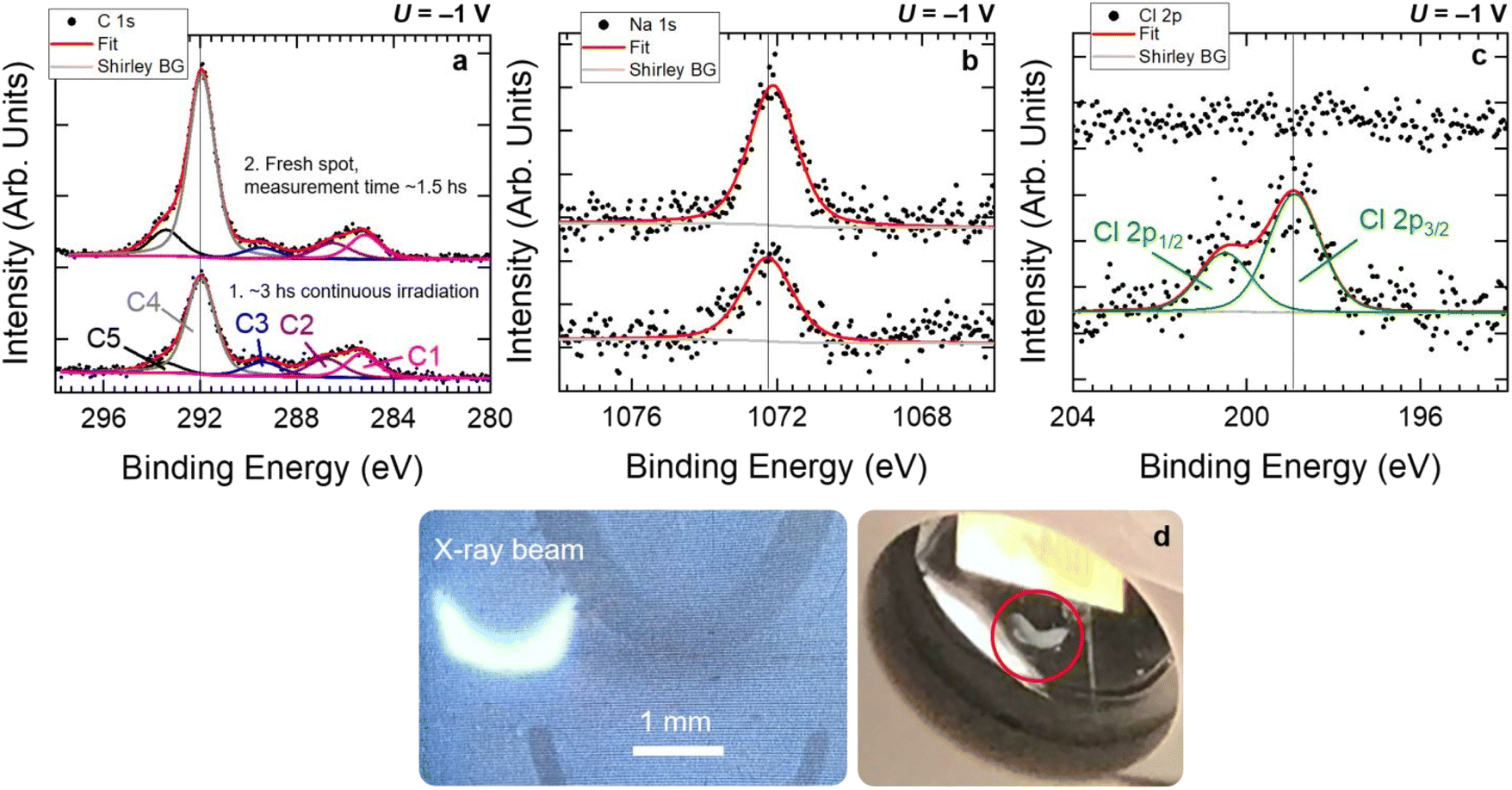Fig. 5 C 1s (a), Na 1s (b), and Cl 2p (c) core level spectra acquired at 3000 eV and at 16–18 mbar of H₂O on Nafion® N115, at an applied potential of −1 V. Bottom spectra were collected after ca. 3 hours of continuous X-ray exposure on the same sample spot. Top spectra were collected afterwards on a fresh spot, within ca. 1.5 hours. Note the strong signal from Cl⁻ detected on the damaged spot. The irradiated area by the X-ray beam after 3 hours of exposure can be visually inspected in (d) (see red circle). For comparison, a digital photograph of the X-ray beam on a phosphorus-coated pad inserted orthogonally to its propagation direction is shown.

Considering that E_ph = 3000 eV is equal to 4.807 × 10⁻¹⁶ J and that Δt is equal to 5400 s (90 minutes exposure) and 10 800 s (3.0 hours exposure), D_E is found to be 8.25 mJ cm⁻² and 16.50 mJ cm⁻², respectively. These values are in line with damage limits reported in the literature for tender X-rays (∼2–10 keV).⁸⁶ Interestingly, under our experimental conditions we observed that an exposure time of about 2 hours, equivalent to a dose of about 11 mJ cm⁻², represents the onset of the degradation of the membranes exposed to the X-rays. The extent of the degradation depends strongly on the chemical composition, volumetric density, and conductivity of the polymers. For N115, the penetration depth of 3000 eV photons is about 3.4 μm, whereas for FAA-3-75 is equal to 12.8 μm (these values were obtained using the database reported in ref. ⁸⁷, using the membrane experimental chemical compositions reported in Table 2 and assuming an incidence angle of 10° between the incoming X-rays and the sample surface. Recall that the penetration depth is defined as the depth into the material measured along the surface normal where the intensity of the X-rays falls to 1/e of its value at the surface). The generation of secondary electrons due to the inelastic scattering of X ray-induced primary photoelectrons off surrounding atoms can lead to the creation of free radicals in polymers. These radicals can mediate the breaking of bonds between the atoms in the polymer chains, leading to the formation of smaller fragments.^86,88 This process is known as scission and can lead to a reduction in the molecular weight of the polymer. As the molecular weight decreases, the mechanical properties of the polymer, such as its strength and elasticity, can also deteriorate. X-ray damage can also lead to the formation of crosslinks in polymers,^86,88 which can instead increase the molecular weight of the polymer. Crosslinking can lead to an increase in the stiffness and hardness of the polymer, but can also make it more brittle and susceptible to cracking. Given the rather complex chemical composition and structure of the investigated membranes, it is difficult to predict which of the described phenomena dominates under our experimental conditions. The use of HAXPES has the advantage that the higher photon energy (and correspondingly, the photoelectron kinetic energy) drastically decreases the secondary electron emission. When combined with ambient pressure conditions, the lower photoionization cross sections also help reduce the environment-dependent radiation damage (i.e., through radiolysis of vapor or gas molecules).⁸⁹ This has the beneficial effect of limiting the radiation-induced damage suffered by the sample under investigation. Nevertheless, after prolonged exposure of the same sample spot to the X-rays, we could observe that a macroscopic degradation of the membrane (Fig. 5d) was accompanied by its inability to retain co-ions, unlike what was observed for pristine sample positions. For the case of the N115 membrane reported in Fig. 5, a chlorine peak could be detected on the near-surface region of the sample (Fig. 5c) after 3 hours of data collection on the same sample location. Hence, we found that an exposure time between 40 and 90 minutes was a good compromise between obtaining a satisfactory signal-to-noise ratio for the collected spectra and ensuring the stability of the membranes during the investigation. Within this period and with the signal-to-noise ratio characterizing the data reported in this study, we were unable to detect any change in the acquired core levels that could indicate changes in the chemical composition of the membrane surface and near surface region. Therefore, we think that the results reported in this work reliably represent the true chemical/physical properties of the membranes under investigation, and that our experimental procedure leads to eventual radiation-induced damage below the detection limit of the technique for the chosen investigation conditions.

3.3. Finite element analysis

To understand the processes that contribute to ion movement in the investigated membranes, 2-D multiphysics simulations based on finite element methods were performed. Detailed descriptions of the 2-D model, governing equations, and boundary conditions are provided in the Experimental section. The diffusivities (i.e. diffusion coefficients) of ions in membranes are important parameters in our simulations. For counter-ions (i.e., Na⁺ in N115 and Cl⁻ in FAA-3-75), the reported diffusivity values in the literature were used (see Table S1†). However, the diffusivity values of co-ions (i.e., Cl⁻ in N115 and Na⁺ in FAA-3-75) are not widely available. Therefore, our in situ AP-HAXPES detection limit (vide supra) was used as a reference to determine the diffusivity values of co-ions. Since our experiments did not detect any Cl⁻ and Na⁺ at the N115/vacuum and FAA-3-75/vacuum interfaces, respectively, their respective atomic concentrations must be lower than our detection limit. We assume a value of 500 ppm for both; using parameters listed in Table 1, this translates to a molar concentration of 0.9 mM for Cl⁻ at the N115/vacuum interface and 0.7 mM for Na⁺ at the FAA-3-75/vacuum interface. Fig. 6a and b show the simulated concentration of Cl⁻ and Na⁺ at the N115/vacuum and FAA-3-75/vacuum interfaces, respectively, as a function of the ion diffusivity after a continuous operation of 4.5 hours at the half-cell OCP. As expected, the concentration increases with increasing diffusivity values until a plateau is reached. We used the diffusivity values at which the co-ions’ concentration at the membrane/vacuum interface is equal to our in situ AP-HAXPES detection limit (red dashed lines in Fig. 6a and b): 1.75 × 10⁻¹³ m² s⁻¹ for the diffusivity of Cl⁻ in N115 and 5.10 × 10⁻¹⁴ m² s⁻¹ for the diffusivity of Na⁺ in FAA-3-75. Although our model is a 2-D one (see Fig. 1), negligible distribution of ion concentrations was found in the y-direction; only distribution profiles along the x-direction at the middle of the cell (i.e., y = 5 mm) are therefore discussed below.

Fig. 6 Simulated concentration of (a) Cl⁻ at the N115/vacuum interface and (b) and Na⁺ at the FAA-3-75/vacuum interface as a function of the respective ion diffusivity after a continuous operation of 4.5 hours at half-cell OCP. The red dashed lines represent an atomic concentration of 500 ppm, which is lower than our in situ AP-HAXPES detection limit.

Fig. 7a shows the simulated concentration profiles of Na⁺ throughout the electrolyte and the N115 membrane at various conditions according to the stages in our AP-HAXPES experiments: half-cell OCP (1.5 hours) followed by the application of +1 V (1.5 hours) and −1 V (1.5 hours). No concentration gradient is observed in both the electrolyte or the membrane, and the application of the potential does not affect the concentration profile. This is consistent with the AP-HAXPES results that show little to no change to the Na⁺ concentration at the N115/vacuum interface (Fig. S10b†). The concentration profiles of Cl⁻ are shown in Fig. 7b. In the electrolyte, the Cl⁻ concentration remains constant at the bulk value (1.0 M), while concentration gradients occur inside the N115 membrane. For all the conditions investigated, the concentration of Cl⁻ at the N115/vacuum interface remains negligible, which is consistent with Cl⁻ being not detected in our AP-HAXPES experiments. The Cl⁻ concentration gradient in the membrane changes with applied potential, but it is not clear whether this is the effect of diffusion (due to the time passed between the OCP and the last applied bias) or ion electromigration. To test this, we compare the Cl⁻ concentration profile at two conditions: (i) OCP for 1.5 h followed by the application of +1 V for 1.5 h and −1 V for 1.5 h and (ii) OCP for 4.5 h (i.e., the same total time as (i)). As shown in Fig. 7c, these two concentration profiles practically fall on top of each other, which indicates that the ion movement into the membrane is driven solely by the diffusion process. The same observations regarding the concentration profile of counter and co-ions are found for the FAA-3-75 membrane, which is shown in Fig. S13.†

Fig. 7 Simulated concentration profile of (a) Na⁺ and (b) Cl⁻ throughout the electrolyte and N115 membrane (see Fig. 1 for the geometry of the model). Three different electrochemical conditions, based on our AP-HAXPES experiments, were considered: (i) half-cell open circuit potential (OCP), (ii) OCP followed by the application of +1 V, and (iii) OCP followed by the application of +1 V and −1 V. (c) Comparison of the simulated concentration profile of Cl⁻ at regions close to and inside the Nafion membrane under the electrochemical condition (iii) above (black circles) and OCP for 4.5 hours (blue line).

4. Discussion

The experimental and theoretical investigations show that the applied bias has no effect on the counter-ion concentration for IEMs used in hybrid liquid/gas electrolyzers, within the time frame of our investigations and the detection limit of AP-HAXPES. In fact, both N115 and FAA-3-75 membranes exhibit surface signals from their corresponding counter-ions (Na⁺ for the CEM N115 and Cl⁻ for the AEM FAA-3-75) irrespective of the potential applied across the membrane in the hybrid liquid/gas cell. The rapid diffusion of sodium into Nafion® has been previously reported upon the immersion of the proton-loaded polymer into sodium iodide solution, which resulted in the replacement of 90% of protons by Na⁺ within 2 min.⁹⁰ A similar behaviour for the FAA-3-75 membrane is expected, with the formation of a quaternary ammonium salt with the chloride counter-ion. The fact that the counter-ion concentration within the near surface region of the membrane is independent of the applied bias points toward an osmotic effect as the dominating driving force for the selective diffusion of counter-ions through the membrane. Such process can be related to the Donnan effect, which is generally used to describe the ionic selectivity of ion exchange membranes without the application of an external field and specifies that the ionic selectivity depends on the presence of the ionized functional groups in the membrane and their corresponding electrostatic interactions with the co- and counter-ions present in solution.^91–93 Due to the constraint of fixed charges/ions, the equilibrium state of the system requires a charge rearrangement to fulfil electroneutrality. Such charge rearrangement results in an unequal ionic distribution on the membrane and solution sides, which leads to a concentration gradient across the membrane. This translates into an osmotic pressure and a potential difference between the membrane sides,⁹² thus influencing the selective rejection of the co-ions in aqueous or polar phases.⁹⁴ Water also plays an important role in the mediation of ion transport in hybrid liquid/gas electrolyzers. For a water-saturated membrane, water desorption is faster than sorption.^95,96 Hence, a continuous diffusion of water from the electrolyte side to the outer triple phase boundary is expected (i.e. water is continuously transferred from the liquid side to the gas phase), thereby constituting an additional driving force for the diffusion of counter-ions through the membrane and their consequent accumulation within the near surface region of the membrane. We therefore conclude that ion electromigration through the membrane induced by the applied external bias in hybrid liquid/gas electrolyzers has little to no effect on the accumulation of counter-ions within the membrane's near surface region. Interestingly, a fast potential switch did not result in any significant reverse ionic diffusion, both from experimental and theoretical findings. Noteworthy, the time that has elapsed after the potential was switched from OCP to the last applied potential seems to be the only factor that determines the concentration of counter-ions within the membrane's near surface region. This is in line with the discussion above, and it suggests that the counter-ions that accumulate non-reversibly at the triple phase boundary can be interpreted as being ionically bonded to the membrane functional groups.

Finally, we want to highlight that when the applied potential favored the diffusion of the counter-ions, i.e. −1 V for Na⁺ in N115 and +1 V for Cl⁻ in FAA-3-75, the extent of the observed BE shift (∼1 eV) matches the magnitude of the applied potential. In the opposite polarity, however, the BE shift is systematically lower (−0.3 eV for N115 and +0.7 eV for FAA-3-75) than the applied potential (+1 V for N115 and −1 V for FAA-3-75), although in the expected direction. This deviation could be a consequence of a polarity-induced ionic rearrangement at the liquid electrolyte/membrane interface. That is, for N115 (FAA-3-75) case, upon positive (negative) polarization of the membrane, Na⁺ (Cl⁻) ions in the electrolyte are displaced in the vicinity of the CE, while Cl⁻ (Na⁺) ions move toward the membrane. Here, they likely accumulate at the liquid electrolyte/N115 (FAA-3-75) interface, since their diffusion through the membrane is rejected by the ionized functional groups in the membranes. Such rearrangement of charges can induce a polarization field that is opposite to the applied electric field and therefore reduces its magnitude, thus possibly explaining the voltage drop across the respective systems. Noteworthy, the observed deviation of ΔBE between the experimental and expected values is consistently lower for Fumasep® FAA-3-75 than for Nafion® N115. Although the cause for such a difference remains unclear, the different functional groups present in the FAA-3-75 and N115 membranes, their charge, and volumetric density likely play a role in the electrostatic interaction between the membrane and the co-ions present in solution. The observed differences in the ΔBE values for the two membranes could be attributed to these varying electrostatic interactions. We acknowledge that exploring the latter would require a theoretical investigation based on a hybrid finite element/molecular dynamic approach that is beyond the scope of this work. Nonetheless, we believe that our model can reasonably provide a qualitative explanation of the observed ΔBE deviation between the two membranes investigated in this work, and could be used by other researchers working with the same type of devices and IEMs to interpret their findings.

5. Conclusion

We characterized selected cation Nafion® 115 and anion Fumasep® FAA-3-PK-75 exchange membranes by means of AP-HAXPES. The use of AP-HAXPES, coupled with customized in situ cells, enabled the in situ characterization of the membranes with photoelectron spectroscopy under applied potential and close to the vapor pressure of water at room temperature. The specific ionic fingerprints of Na⁺ for N115 and Cl⁻ for FAA-3-75 measured with AP-HAXPES under polarization conditions are unambiguous and the respective ions appear to readily out-diffuse at the equilibrium conditions (half-cell OCP), irrespective of the applied bias polarity and magnitude. This experimental observation is supported by finite element analysis conducted on the same time scale and using the same (simulated) detection limit as the experimental investigation. Our combined experimental and theoretical findings suggest that the electrostatic interactions between the ions and the ionized functional groups on the membrane, supported by the concomitant diffusion of water, dominate the diffusion of counter-ions through polymer membranes in hybrid liquid/gas electrolyzers. Perhaps surprisingly, electromigration induced by the applied bias seems not playing a central role in these type of configurations. In addition, by using in situ AP-HAXPES, we were able to directly detect unwanted polarization fields at the interface between the liquid electrolyte and the membrane. This occurred when the polarity of the applied potential was the same as the charge of the co-ions (i.e., the charge of the ionized functional groups present in the IEMs). The generation of such polarization fields was attributed to the accumulation of co-ions at the liquid electrolyte/membrane interface, resulting from their rejection and consequent inability to diffuse through the membrane. This leads to a loss in the cell voltage, with detrimental effects on the overall performance and reaction selectivity of the hybrid liquid/gas electrolyzer.

This work illustrates a potential path for the study of IEMs using in situ AP-HAXPES and the monitoring of their physical/chemical properties under realistic working conditions. Such studies contribute to a deeper understanding of IEMs behaviour, which is essential to enable their optimization and tailor their design. Our findings can contribute to the rationalization of the (photo)electrochemical performance of hybrid liquid/gas electrolyzers, a configuration that is increasingly utilized for various electrochemical reactions, particularly the reduction of CO₂ and nitrogen.

Author contributions

The manuscript was written through contributions of all authors. All authors have given approval to the final version of the manuscript.

Conflicts of interest

The authors declare no competing interests.

Acknowledgements

This project was partly supported by the Federal Ministry of Education and Research (BMBF) through the CatLab project (Förderkennzeichen 03EW0015A). The SpAnTeX end-station operates at the BESSY II synchrotron facility within the Berlin joint laboratory for ElectroChemical interfaces (BElChem), established between the Helmholtz-Zentrum Berlin (HZB) and the Fritz Haber Institute der Max Planck Gesellschaft (FHI-MPG). The development of the SpAnTeX end-station was supported by the Helmholtz Association through the Helmholtz Energy Materials Foundry (HEMF, GZ 714-48172-21/1) and partly by the BMBF through the CatLab project (Förderkennzeichen 03EW0015A). The authors would like to gratefully acknowledge the staff at the BESSY II synchrotron facility, in particular Dr Roberto F. Duarte and Marcel Mertin for their technical support during beam time. We would also like to acknowledge Katrin Tietz, Thorsten Wagner, Marvin Bruns, and Mohammad Khalf (HZB) for their technical support and for the fabrication of the devices reported in this work. We thank Analice T. Silva Diniz, Dr Matias Berasategui, Dr Matthew T. Mayer, and Dr David E. Starr for the valuable discussions.

References

1. J. Ran, L. Wu, Y. He, Z. Yang, Y. Wang, C. Jiang, L. Ge, E. Bakangura and T. Xu, J. Membr. Sci., 2017, 522, 267–291.
2. S. Z. Oener, S. Ardo and S. W. Boettcher, ACS Energy Lett., 2017, 2, 2625–2634.
3. L. Dong and Y. Zhao, J. Mater. Chem. A, 2020, 8, 16738–16746.
4. G. Segev, J. Kibsgaard, C. Hahn, Z. J. Xu, W.-H. (Sophia) Cheng, T. G. Deutsch, C. Xiang, J. Z. Zhang, L. Hammarström, D. G. Nocera, A. Z. Weber, P. Agbo, T. Hisatomi, F. E. Osterloh, K. Domen, F. F. Abdi, S. Haussener, D. J. Miller, S. Ardo, P. C. McIntyre, T. Hannappel, S. Hu, H. Atwater, J. M. Gregoire, M. Z. Ertem, I. D. Sharp, K.-S. Choi, J. S. Lee, O. Ishitani, J. W. Ager, R. R. Prabhakar, A. T. Bell, S. W. Boettcher, K. Vincent, K. Takanabe, V. Artero, R. Napier, B. R. Cuenya, M. T. M. Koper, R. V. D. Krol and F. Houle, J. Phys. D: Appl. Phys., 2022, 55, 323003.
5. M. Tedesco, H. V. M. Hamelers and P. M. Biesheuvel, J. Membr. Sci., 2016, 510, 370–381.
6. S. Zhao, in Waste to Renewable Biohydrogen, ed. Q. Zhang, C. He, J. Ren and M. Goodsite, Academic Press, 2021, pp. 139–177.
7. M. Park, J. Ryu, W. Wang and J. Cho, Nat. Rev. Mater., 2016, 2, 1–18.
8. H. Strathmann, A. Grabowski and G. Eigenberger, Ind. Eng. Chem. Res., 2013, 52, 10364–10379.
9. G. A. El-Nagar, F. Haun, S. Gupta, S. Stojkovikj and M. T. Mayer, Unintended cation crossover influences CO2 reduction activity in Cu-based zero-gap electrolysers, Nat. Commun., 2023, 14, 2062.
10. V. M. Palakkal, J. E. Rubio, Y. J. Lin and C. G. Arges, ACS Sustainable Chem. Eng., 2018, 6, 13778–13786.
11. D. A. Salvatore, C. M. Gabardo, A. Reyes, C. P. O'Brien, S. Holdcroft, P. Pintauro, B. Bahar, M. Hickner, C. Bae, D. Sinton, E. H. Sargent and C. P. Berlinguette, Nat. Energy, 2021, 6, 339–348.
12. F. Nandjou and S. Haussener, J. Phys. D: Appl. Phys., 2017, 50, 124002.
13. M. P. Rodgers, L. J. Bonville, H. R. Kunz, D. K. Slattery and J. M. Fenton, Chem. Rev., 2012, 112, 6075–6103.
14. S. Garg, C. G. Rodriguez, T. E. Rufford, J. R. Varcoe and B. J. Seger, Energy Environ. Sci., 2022, 15, 4440–4469.
15. A. Yaroshchuk and M. L. Bruening, J. Membr. Sci., 2017, 523, 361–372.
16. A. K. Friedman, W. Shi, Y. Losovyj, A. R. Siedle and L. A. Baker, J. Electrochem. Soc., 2018, 165, H733.
17. M. Schulze, M. Lorenz, N. Wagner and E. Gülzow, Fresenius. J. Anal. Chem., 1999, 365, 106–113.
18. M. A. Vandiver, B. R. Caire, T. P. Pandey, Y. Li, S. Seifert, A. Kusoglu, D. M. Knauss, A. M. Herring and M. W. Liberatore, J. Membr. Sci., 2016, 497, 67–76.
19. M. G. Marino, J. P. Melchior, A. Wohlfarth and K. D. Kreuer, J. Membr. Sci., 2014, 464, 61–71.
20. F. Foglia, V. Garcia Sakai, S. Lyonnard and P. F. McMillan, J. Non-Cryst. Solids: X, 2022, 13, 100073.
21. F. Foglia, Q. Berrod, A. J. Clancy, K. Smith, G. Gebel, V. G. Sakai, M. Appel, J.-M. Zanotti, M. Tyagi, N. Mahmoudi, T. S. Miller, J. R. Varcoe, A. P. Periasamy, D. J. L. Brett, P. R. Shearing, S. Lyonnard and P. F. McMillan, Nat. Mater., 2022, 21, 555–563.
22. M. Vijayakumar, M. S. Bhuvaneswari, P. Nachimuthu, B. Schwenzer, S. Kim, Z. Yang, J. Liu, G. L. Graff, S. Thevuthasan and J. Hu, J. Membr. Sci., 2011, 366, 325–334.
23. K. Isegawa, T. Nagami, S. Jomori, M. Yoshida and H. Kondoh, Phys. Chem. Chem. Phys., 2016, 18, 25183–25190.
24. L. Yu, Y. Takagi, T. Nakamura, T. Sakata, T. Uruga, M. Tada, Y. Iwasawa, S. Masaoka and T. Yokoyama, J. Phys. Chem. C, 2019, 123, 603–611.
25. P. Aydogan Gokturk, R. Sujanani, J. Qian, Y. Wang, L. E. Katz, B. D. Freeman and E. J. Crumlin, Nat. Commun., 2022, 13, 5880.
26. C. Liu, J. Liu, Y. Han, Z. Wang, H. Zhang, X. Xie, B. Yang and Z. Liu, J. Chem. Phys., 2023, 158, 071101.
27. M. F. Lichterman, S. Hu, M. H. Richter, E. J. Crumlin, S. Axnanda, M. Favaro, W. Drisdell, Z. Hussain, T. Mayer, B. S. Brunschwig, N. S. Lewis, Z. Liu and H.-J. Lewerenz, Energy Environ. Sci., 2015, 8, 2409–2416.
28. M. Favaro, B. Jeong, P. N. Ross, J. Yano, Z. Hussain, Z. Liu and E. J. Crumlin, Nat. Commun., 2016, 7, 12695.
29. M. Favaro, C. Valero-Vidal, J. Eichhorn, F. M. Toma, P. N. Ross, J. Yano, Z. Liu and E. J. Crumlin, J. Mater. Chem. A, 2017, 5, 11634–11643.
30. M. Favaro, F. F. Abdi, M. Lamers, E. J. Crumlin, Z. Liu, R. van de Krol and D. E. Starr, J. Phys. Chem. B, 2018, 122, 801–809.
31. A. Shavorskiy, X. Ye, O. Karslıoğlu, A. D. Poletayev, M. Hartl, I. Zegkinoglou, L. Trotochaud, S. Nemšák, C. M. Schneider, E. J. Crumlin, S. Axnanda, Z. Liu, P. N. Ross, W. Chueh and H. Bluhm, J. Phys. Chem. Lett., 2017, 8, 5579–5586.
32. O. Brummel, Y. Lykhach, M. Ralaiarisoa, M. Berasategui, M. Kastenmeier, L. Fusek, A. Simanenko, W. Gu, P. C. J. Clark, R. Yivlialin, M. J. Sear, J. Mysliveček, M. Favaro, D. E. Starr and J. Libuda, J. Phys. Chem. Lett., 2022, 13, 11015–11022.
33. J. Lee, W. Lee, K. H. Ryu, J. Park, H. Lee, J. H. Lee and K. T. Park, Green Chem., 2021, 23, 2397–2410.
34. W. Lee, Y. E. Kim, M. H. Youn, S. K. Jeong and K. T. Park, Angew. Chem., Int. Ed., 2018, 57, 6883–6887.
35. B. De Mot, M. Ramdin, J. Hereijgers, T. J. H. Vlugt and T. Breugelmans, ChemElectroChem, 2020, 7, 3839–3843.
36. S. van Bavel, S. Verma, E. Negro and M. Bracht, ACS Energy Lett., 2020, 5, 2597–2601.
37. V. Streibel, M. Hävecker, Y. Yi, J. J. Velasco Vélez, K. Skorupska, E. Stotz, A. Knop-Gericke, R. Schlögl and R. Arrigo, Top. Catal., 2018, 61, 2064–2084.
38. A. Lim, H. Kim, D. Henkensmeier, S. Jong Yoo, J. Young Kim, S. Young Lee, Y.-E. Sung, J. H. Jang and H. S. Park, J. Ind. Eng. Chem., 2019, 76, 410–418.
39. M. Carmo, G. Doubek, R. C. Sekol, M. Linardi and A. D. Taylor, J. Power Sources, 2013, 230, 169–175.
40. A. Marinkas, I. Struźyńska-Piron, Y. Lee, A. Lim, H. S. Park, J. H. Jang, H.-J. Kim, J. Kim, A. Maljusch, O. Conradi and D. Henkensmeier, Polymer, 2018, 145, 242–251.
41. H. Khalid, M. Najibah, H. S. Park, C. Bae and D. Henkensmeier, Membranes, 2022, 12, 989.
42. M. A. Hickner, A. M. Herring and E. B. Coughlin, J. Polym. Sci., Part B: Polym. Phys., 2013, 51, 1727–1735.
43. W. Wei, J. Xu, W. Chen, L. Mi and J. Zhang, J. Mater. Chem. A, 2022, 10, 2637–2671.
44. M. M. Ayyub, M. Chhetri, U. Gupta, A. Roy and C. N. R. Rao, Chem. - Eur. J., 2018, 24, 18455–18462.
45. S. Dresp, F. Dionigi, M. Klingenhof and P. Strasser, ACS Energy Lett., 2019, 4, 933–942.
46. M. Jadwiszczak, K. Jakubow-Piotrowska, P. Kedzierzawski, K. Bienkowski and J. Augustynski, Adv. Energy Mater., 2020, 10, 1903213.
47. L. N. Nthunya, M. F. Bopape, O. T. Mahlangu, B. B. Mamba, B. Van der Bruggen, C. A. Quist-Jensen and H. Richards, J. Environ. Manage., 2022, 301, 113922.
48. E. Borgardt, L. Giesenberg, M. Reska, M. Müller, K. Wippermann, M. Langemann, W. Lehnert and D. Stolten, Int. J. Hydrogen Energy, 2007, 44, 23556–23567.
49. Y. Chen, J. Zhao, C. Jin, Y. Ke, D. Li and Z. Wang, Membranes, 2022, 12, 645.
50. D. W. Baker and W. Haynes, Engineering Statics: Open and Interactive, Colorado State University Digital Learning Initiative, and the Colorado State University Libraries, 2023.
51. Metric fine ISO, https://www.tribology-abc.com/calculators/metric-fine-iso.htm, accessed March 25, 2023.
52. Böllhoff, The Manual of Fastening Technology, 5th edn, 2007.
53. M. Favaro, P. C. J. Clark, M. J. Sear, M. Johansson, S. Maehl, R. van de Krol and D. E. Starr, Surf. Sci., 2021, 713, 121903.
54. F. Schaefers, M. Mertin and M. Gorgoi, Rev. Sci. Instrum., 2007, 78, 123102.
55. D. R. Lide, CRC Handbook of Chemistry and Physics, 85th edn, CRC Press, 2004.
56. M. B. Trzhaskovskaya, V. I. Nefedov and V. G. Yarzhemsky, At. Data Nucl. Data Tables, 2001, 77, 97–159.
57. M. B. Trzhaskovskaya, V. I. Nefedov and V. G. Yarzhemsky, At. Data Nucl. Data Tables, 2002, 82, 257–311.
58. S. Tanuma, C. J. Powell and D. R. Penn, Surf. Interface Anal., 2003, 35, 268–275.
59. W. Smekal, W. S. M. Werner and C. J. Powell, Surf. Interface Anal., 2005, 37, 1059–1067.
60. X. Wu, C. Villevieille, P. Novák and M. E. Kazzi, Phys. Chem. Chem. Phys., 2018, 20, 11123–11129.
61. S. Axnanda, E. J. Crumlin, B. Mao, S. Rani, R. Chang, P. G. Karlsson, M. O. M. Edwards, M. Lundqvist, R. Moberg, P. Ross, Z. Hussain and Z. Liu, Sci. Rep., 2015, 5, 9788.
62. S. Alinejad, M. Inaba, J. Schröder, J. Du, J. Quinson, A. Zana and M. Arenz, J. Phys.: Energy, 2020, 2, 024003.
63. Fumasep FAA-3-PK-75, https://www.fuelcellstore.com/fumasep-faa-3-pk-75, accessed January 10, 2023.
64. D. Henkensmeier, M. Najibah, C. Harms, J. Žitka, J. Hnát and K. Bouzek, J. Electrochem. Energy Convers. Storage, 2021, 18(2), 024001.
65. A. Basile, K. Ghasemzadeh and A. Iulianelli, Current Trends and Future Developments on (Bio-) Membranes: Transport Phenomena in Membranes, Elsevier, 2021.
66. S. Slade, S. A. Campbell, T. R. Ralph and F. C. Walsh, J. Electrochem. Soc., 2002, 149, A1556.
67. T. A. Jr Zawodzinski, M. Neeman, L. O. Sillerud and S. Gottesfeld, J. Phys. Chem., 1991, 95, 6040–6044.
68. K. A. Mauritz and R. B. Moore, Chem. Rev., 2004, 104, 4535–4586.
69. H. Shinotsuka, S. Tanuma, C. J. Powell and D. R. Penn, Surf. Interface Anal., 2015, 47, 871–888.
70. N. Comini, T. Huthwelker, J. T. Diulus, J. Osterwalder and Z. Novotny, J. Vac. Sci. Technol., A, 2021, 39, 043203.
71. E. A. Hoffmann, Z. A. Fekete, L. S. Korugic-Karasz, F. E. Karasz and E. Wilusz, J. Polym. Sci., Part A: Polym. Chem., 2004, 42, 551–556.
72. R. Chaney and G. Barth, Fresenius' Z. Anal. Chem., 1987, 329, 143–146.
73. E. Damian Risberg, L. Eriksson, J. Mink, L. G. M. Pettersson, M. Yu. Skripkin and M. Sandström, Inorg. Chem., 2007, 46, 8332–8348.
74. L. Yan, P. B. Balbuena and J. M. Seminario, J. Phys. Chem. A, 2006, 110, 4574–4581.
75. Z. Zuo, Y. Fu and A. Manthiram, Polymers, 2012, 4, 1627–1644.
76. K. Isegawa, D. Kim and H. Kondoh, RSC Adv., 2018, 8, 38204–38209.
77. M. Favaro, G. A. Rizzi, S. Nappini, E. Magnano, F. Bondino, S. Agnoli and G. Granozzi, Surf. Sci., 2016, 646, 132–139.
78. J. F. Moulder, Handbook of X-Ray Photoelectron Spectroscopy: A Reference Book of Standard Spectra for Identification and Interpretation of XPS Data, Physical Electronics Division, Perkin-Elmer Corporation, 1992.
79. A. G. Divekar, A. M. Park, Z. R. Owczarczyk, S. Seifert, B. S. Pivovar and A. M. Herring, ECS Trans., 2017, 80, 1005.
80. N. Ziv, W. E. Mustain and D. R. Dekel, ChemSusChem, 2018, 11, 1136–1150.
81. U. Krewer, C. Weinzierl, N. Ziv and D. R. Dekel, Electrochim. Acta, 2018, 263, 433–446.
82. J. Yan and M. A. Hickner, Macromolecules, 2010, 43, 2349–2356.
83. D. Zhang, J. Shi, W. Zi, P. Wang and S. (Frank) Liu, ChemSusChem, 2017, 10, 4324–4341.
84. H. Tissot, J.-J. Gallet, F. Bournel, G. Olivieri, M. G. Silly, F. Sirotti, A. Boucly and F. Rochet, Top. Catal., 2016, 59, 605–620.
85. A. G. Shard, Surf. Interface Anal., 2014, 46, 175–185.
86. S. A. Vaselabadi, D. Shakarisaz, P. Ruchhoeft, J. Strzalka and G. E. Stein, J. Polym. Sci., Part B: Polym. Phys., 2016, 54, 1074–1086.
87. CXRO X-Ray Interactions With Matter, https://henke.lbl.gov/optical_constants/, accessed March 25, 2023.
88. T. Coffey, S. G. Urquhart and H. Ade, J. Electron Spectrosc. Relat. Phenom., 2002, 122, 65–78.
89. R. S. Weatherup, C. H. Wu, C. Escudero, V. Pérez-Dieste and M. B. Salmeron, J. Phys. Chem. B, 2018, 122, 737–744.
90. M. Lopez, B. Kipling and H. L. Yeager, Anal. Chem., 1976, 48, 1120–1122.
91. F. G. Donnan, Z. Elektrochem. Angew. Phys. Chem., 1911, 17, 572–581.
92. F. G. Donnan, Chem. Rev., 1924, 1, 73–90.
93. F. G. Donnan, J. Membr. Sci., 1995, 100, 45–55.
94. S. Sarkar, A. K. SenGupta and P. Prakash, Environ. Sci. Technol., 2010, 44, 1161–1166.
95. P. Majsztrik, B. Satterfield, A. Bocarsly and J. B. Benziger, ECS Trans., 2007, 11, 609.
96. P. Majsztrik, A. Bocarsly and J. Benziger, J. Phys. Chem. B, 2008, 112, 16280–16289.

---

Footnote

† Electronic supplementary information (ESI) available. See DOI: https://doi.org/10.1039/d3ta02050a

---