DOI:
10.1039/D3SM00351E
(Paper)
Soft Matter, 2023,
19, 6929-6944
Probing the elastic response of lipid bilayers and nanovesicles to leaflet tensions via volume per lipid†
Received
18th March 2023
, Accepted 11th August 2023
First published on 14th August 2023
Abstract
Biological and biomimetic membranes are based on lipid bilayers, consisting of two monolayers or leaflets. One important but challenging physical parameter of these membranes is their tension. For a long time, this tension was explicitly or implicitly taken to be the bilayer tension, acting on the whole bilayer membrane. More recently, it has been realized that it is useful to decompose the bilayer tension into two leaflet tensions and that these tensions are accessible to molecular dynamics simulations. To divide the bilayer up into two leaflets, it is necessary to introduce a midsurface that defines the spatial extent of the two leaflets. In previous studies, this midsurface was obtained from the density profiles across the bilayer and was then used to compute the molecular area per lipid. Here, we develop an alternative approach based on three-dimensional Voronoi tessellation and molecular volume per lipid. Using this volume-based approach, we determine the reference states with tensionless leaflets as well as the optimal volumes and areas per lipid. The optimal lipid volumes have practically the same value in both leaflets, irrespective of the size and curvature of the nanovesicles, whereas the optimal lipid areas are different for the two leaflets and depend on the vesicle size. In addition, we introduce lateral volume compressibilities to describe the elastic response of the lipid volume to the leaflet tensions. We show that the outer leaflet of a nanovesicle is more densely packed and less compressible than the inner leaflet and that this difference becomes more pronounced for smaller vesicles.
1 Introduction
Biological membranes are an essential part of the living cell. On the molecular scale, each biological membrane consists of a specific and complex assortment of many different lipids and membrane proteins. However, in spite of this chemical diversity, the basic building block of all biomembranes is provided by a fluid bilayer of lipid molecules.1–3 Therefore, the simplest biomimetic membranes are lipid bilayers in their fluid state, without any proteins.4–7 One important but challenging physical parameter of these membranes is their tension. For a long time, the experimentally and theoretically studied tension was taken to be the bilayer tension that acts within the whole bilayer membrane. A widely used method to measure the bilayer tension experimentally is provided by micropipette aspiration, which has been used for different cell types such as red blood cells,8,9 neutrophils, i.e., certain types of white blood cells,9,10 and fibroblasts11 as well as for giant unilamellar vesicles.12,13 The aspiration method can be combined with magnetic14 and optical tweezers15–17 to pull membrane nanotubes from the cells and vesicles. By modifying the externally applied forces exerted by the magnetic and optical tweezers, one can directly control the bilayer tension within the cell and vesicle membranes. For neutrophils, the bilayer tension was identified with the cortical tension generated by the actomyosin cortex.18–20 For fibroblasts, this tension was decomposed into the cortical tension and another tension that remains after the cortex has been disassembled chemically.11 In the theory of curvature elasticity, the bilayer tension is conjugate to the total membrane area and can be used as a Lagrange multiplier to compute the bending energy under the constraint of constant area.21–23 Strong adhesion of vesicles to a substrate surface leads to adhesion-induced tension and to apparent (or effective) contact angles,24 which can be directly observed in the light microscope25,26 and used to stabilize networks of adhering vesicles connected by nanotubes.27,28
In molecular dynamics simulations as used here, the bilayer tension is obtained by computing the stress profile across the bilayer membrane and by integrating this profile along a coordinate perpendicular to the bilayer.29,30 When the bilayer is divided up into its two leaflets, the bilayer tension Σ is decomposed into two leaflet tensions, Σ1 and Σ2, with Σ = Σ1 + Σ2.30–34 Each leaflet tension can be positive or negative depending on the number of lipids that are assembled in the leaflet. A positive leaflet tension implies that the leaflet is stretched whereas a negative leaflet tension describes a compressed leaflet. Furthermore, for a given number of lipids, the bilayer exhibits a unique reference state, in which both leaflet tensions vanish, Σ1 = Σ2 = 0.
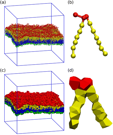
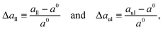
Here, we examine both planar bilayers and bilayers that form spherical nanovesicles as shown in Fig. 1. These bilayer systems differ in their membrane curvature. The mean curvature of the planar bilayer vanishes whereas the mean curvature of a nanovesicle is equal to the inverse vesicle radius. Thus, the smallest nanovesicle in Fig. 1b has the largest mean curvature.
 |
| | Fig. 1 Simulation snapshots of planar bilayer and spherical nanovesicles with vanishing leaflet tensions: (a) cross-section of planar bilayer containing Nlip = 1682 lipids, with a lateral extension of about 26 nm; (b)–(e) Half cuts of nanovesicles assembled from Nlip = 1500 lipids in (b); 2525 lipids in (c); 6312 lipids in (d); and 10![[thin space (1/6-em)]](https://www.rsc.org/images/entities/char_2009.gif) 100 lipids in (e). The diameter of these vesicles varies from 14 nm in (b) to 37 nm in (e). Color code for lipids: Green head groups and blue hydrocarbon chains in the lower and inner leaflets; red heads and yellow chains in the upper and outer leaflets. All bilayer systems are surrounded by plenty of water molecules (not shown). 100 lipids in (e). The diameter of these vesicles varies from 14 nm in (b) to 37 nm in (e). Color code for lipids: Green head groups and blue hydrocarbon chains in the lower and inner leaflets; red heads and yellow chains in the upper and outer leaflets. All bilayer systems are surrounded by plenty of water molecules (not shown). | |
Starting from the reference states with vanishing leaflet tensions, we explore certain types of elastic deformations. For planar bilayers, we distinguish elastic deformations corresponding to ‘equal leaflet tensions’ (ELTs) from deformations with ‘opposite leaflet tensions’ (OLTs). During an ELT deformation with Σ2 = Σ1, the two leaflets of the bilayer are stretched or compressed in the same manner. The OLT deformations with Σ2 = −Σ1, on the other hand, are obtained from the reference state by reshuffling lipids from one leaflet to the other, while the total lipid number of the bilayer is kept constant. The same procedure defines OLT deformations of vesicle bilayers. It turns out, however, that ELT deformations of vesicle bilayers cannot be obtained via a simple procedure. Therefore, for nanovesicles, we replace ELT deformations by elastic deformations arising from vesicle inflation or deflation (VID), corresponding to an increase or reduction of the vesicle volume.
Planar bilayers are convenient from a computational point of view because their reference state with vanishing leaflet tensions is provided by a symmetric bilayer that involves the same number of lipids in both leaflets. Furthermore, for a planar and symmetric bilayer, vanishing bilayer tension with Σ = Σ1 + Σ2 = 0 implies vanishing leaflet tensions with Σ1 = Σ2 = 0. Planar lipid bilayers can be experimentally prepared as black lipid membranes35 and pore-spanning membranes36 but both model membranes have a relatively short lifetime because they experience large bilayer tensions arising from the adhesion to the underlying substrate surface. Nanovesicles, on the other hand, are built up from freely suspended bilayers in aqueous solution which form closed surfaces to avoid bilayer edges. After osmotic equilibration, the bilayers of these nanovesicles can attain a state of vanishing bilayer tension.
Both synthetic and cellular nanovesicles have been experimentally studied. Synthetic nanovesicles are assembled from lipid molecules, using a variety of preparation methods,37,38 which produce a wide range of vesicle sizes. We will consider nanovesicles with diameters below 50 nm as in Fig. 1b–e, which have emerged as promising modules for lipid nanotechnology. Indeed, these vesicles have been shown to provide potent platforms for dermal and transdermal drug delivery.39–43 In particular, they have been applied to a variety of skin diseases such as skin cancer44 and psoriasis.45 More recently, such nanovesicles have emerged as nanocarriers for the packaging and delivery of small interfering RNA therapeutics, used to silence various pathways of gene expression,46–48 and for the delivery of mRNA vaccines, which became crucial during the COVID-19 pandemic.47,49,50
On the other hand, cellular nanovesicles such as exosomes and extracellular vesicles are released from almost every type of living cell51 and are crucial for the chemical communication between the cells. These vesicles have been proposed as possible biomarkers for diseases52,53 and as potential drug delivery systems.54,55
Our paper is organized as follows. In Section 2.1, we describe the fluid-elastic behavior of planar bilayers. We first discuss the area per lipid in the two bilayer leaflets as well as the two leaflet tensions. To compute the leaflet tensions for a certain planar bilayer, we need to determine its midplane. We introduce a new protocol, called VORON, for the computation of this midplane. The protocol is based on the volumes of the coarse-grained molecules as determined by Voronoi tessellation. The two leaflet tensions are then used to define a two-dimensional parameter space for all planar bilayer states. In this parameter space, we focus on two orthogonal paths, which describe ELT and OLT deformations. We determine the optimal area per lipid as well as the area compressibility and show that the area compressibility modulus is different for ELT and OLT deformations. In addition, we use the VORON protocol to determine the optimal volume per lipid as well as the lateral volume compressibility moduli of the two leaflets. The latter moduli describe the elastic response of the lipid volumes to the leaflet tensions.
The fluid-elastic behavior of nanovesicles is studied in Section 2.2. We vary the mean curvature of the nanovesicles as in Fig. 1 and determine the curvature dependence of the elastic properties of the vesicle bilayers. First, we generalize the VORON protocol to nanovesicles and describe how this protocol can be used to compute the midsurface of the vesicle bilayers and to determine the areas per lipid from the volumes per lipid. We focus on two elastic deformations of the vesicle bilayers as provided by OLT deformations with Σ2 = −Σ1 and by those arising from vesicle inflation and deflation (VID). We use two previously described methods to estimate the optimal area per lipid and show that these two methods predict qualitatively different curvature dependencies for the optimal area per lipid in the two leaflets. The area compressibility modulus, on the other hand, is found to be quite similar for the two methods. We then apply three-dimensional Voronoi tessellation to the vesicle bilayers and determine the optimal volume per lipid as well as the lateral volume compressibilities within the two leaflets. The optimal lipid volume is found to be very similar in the two leaflets whereas their lateral volume compressibilities are quite different, with the outer leaflet being less compressible than the inner one. We also show that our approach based on Voronoi tessellation provides a simpler and unique method to compute the midsurface radius of the vesicle bilayer. Because the value of this radius is essential in order to decompose the bilayer tension into two leaflet tensions, the Voronoi tessellation greatly facilitate this decomposition. Our study demonstrates that all nanovesicles possess outer leaflets that are more densely packed and less compressible than the inner leaflets. In addition, we also show that both the area and the lateral volume compressibilities of the outer leaflets increase with the mean curvature of the vesicles.
2 Results
2.1 Elastic behavior of planar bilayers
2.1.1 Areas per lipid and leaflet tensions.
We first look at planar bilayers which consist of a lower and an upper leaflet, for which we use the subscripts ll and ul, respectively. We assemble Nll and Nul lipids in these two leaflets, using a simulation box with a certain base area A‖. The (projected) areas per lipid, all and aul, in the two leaflets are then given by| |  | (1) |
When both leaflets are tensionless as in Fig. 1a, the two areas per lipid attain the optimal (or relaxed) values a0ll and a0ul = a0ll. The equality between the two optimal areas per lipid follows from the symmetry of a planar bilayer with the same number of lipids in each leaflet. The bilayer with tensionless leaflets provides the reference system for the bilayer system under consideration. The reference system for the planar bilayer in Fig. 1a, is assembled from Nul = Nll = 841 lipids. An oblique view of this symmetric and tensionless bilayer is displayed in Fig. 2a further below. Note that the areas per lipid in the two leaflets, as given by eqn (1) for a planar bilayer, do not require any decomposition of this bilayer into its two leaflets.
 |
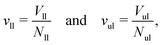
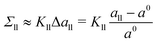
| | Fig. 2 Three-dimensional Voronoi tessellation of the molecular model built up from different types of beads: (a) conformation of planar bilayer with tensionless leaflets and Nll = Nul = 841. The lipids in the lower leaflet have green head groups and blue chain beads; the lipids in the upper leaflet have red head groups and yellow chain beads; (b) typical conformation of a single lipid molecule within the upper leaflet in ball-and-stick representation; (c) Polyhedral Voronoi cells assigned to each bead of the bilayer in panel a; and (d) Voronoi cells assigned to each bead of the lipid molecule in panel b. | |
2.1.2 Midplane separating the two bilayer leaflets.
On the other hand, to calculate the leaflet tensions, we need to decompose the bilayer tension into the contributions from its two leaflets. This decomposition is based on the bilayer's midplane, which represents the molecular interface between the two leaflets and divides the bilayer up into these leaflets.31–33 In the planar bilayer simulations, we impose periodic boundary conditions in the x- and y-directions parallel to the bilayer and denote the Cartesian coordinate perpendicular to it by z. The location of the midplane is then fully characterized by its z-value, z = zmid, see eqn (47) in the Methods section.
For symmetric planar bilayers, which contain the same number of lipids in both leaflets, the midplane coincides with the plane of symmetry. Thus, for a symmetric bilayer, any density profile, ρ = ρ(z), across the bilayer is mirror symmetric with respect to z = zmid. This symmetry applies both to the reference state with tensionless leaflets and to all ELT deformations of this reference state. On the other hand, this symmetry is lost for asymmetric bilayers with a different number of lipids in the two leaflets and, in particular, for all OLT deformations of the reference state.
Several protocols have been previously developed in order to determine the midplane location for asymmetric bilayers.31–33 The simplest protocol, denoted by CHAIN, is to identify the location of the midplane with the z-value, at which the density of the hydrocarbon chains has an extremum. In the coarse-grained molecular dynamics simulations used here, this extremum is a maximum. For the coarse-grained Martini force field, the extremum of the chain density is a minimum.56 In the following, we will introduce a new protocol, called VORON, to compute the midplane location for asymmetric bilayers. This protocol uses Voronoi tessellation to compute the volumes of the coarse-grained molecules and will be applied to both planar bilayers and to the spherical bilayers of nanovesicles.
2.1.3 Molecular volumes from Voronoi tessellation.
To unambiguously calculate the volumes occupied by the coarse-grained molecules, we use three-dimensional Voronoi tessellation. As explained in the Methods section, the molecules are built up from different types of spherical beads. The Voronoi tessellation method assigns a polyhedral cell to each bead, such that all points in this cell are closer to the center of the chosen bead than to the center of any other bead. In Fig. 2, we provide examples for the tessellation of a planar bilayer conformation and for the tessellation of an individual lipid molecule. The Voronoi tessellation is performed within the LAMMPS package,57 which uses the Voro++ library.58
The volume of each Voronoi cell can be calculated using the coordinates of its vertices. Summing up the volumes of those polyhedral cells that belong to a particular subcompartment of the system, we get the volume VlW of the water subcompartment below the bilayer, the volume Vll of the lower leaflet, the volume Vul of the upper leaflet, and the volume VuW of the water subcompartment above the bilayer. The volumes per lipid in the lower and upper leaflet of the planar bilayer are then obtained by
| |  | (2) |
dividing the leaflet volume of each leaflet by the number of lipids assembled in this leaflet.
2.1.4 Midplane location from subcompartment volumes.
Using the volumes of the different subcompartments as determined by Voronoi tessellation, we can now define the VORON protocol to compute the midplane location zmid. The z-coordinate perpendicular to the planar bilayer is taken to vary within the range −Lz ≤ z ≤ + Lz and the base area is denoted by A‖ as before. The geometry of the simulation box then implies| | | (Lz + zmid)A‖ = Vll + VlW | (3) |
where Vll and VlW are the volumes of the lower leaflet and of the water subcompartment below this leaflet as previously mentioned. Likewise, the z-coordinate zmid of the midplane can be obtained via| | | (Lz − zmid)A‖ = Vul + VuW | (4) |
in terms of the volumes Vul and VuW corresponding to the upper leaflet and to the upper water subcompartment. The two relationships in eqn (3) and (4) both determine the midplane coordinate z = zmid in terms of known geometric parameters, giving identical values within the numerical accuracy.
2.1.5 Optimal area per lipid and area compressibilities.
As mentioned, the reference states with tensionless leaflets are provided by symmetric bilayers with Nul = Nll, that is, with the same number of lipids in the lower and upper leaflet. For Nul = Nll = 841, our simulations lead to the numerical values| | | a0ll = a0ul = (1.219 ± 0.002)d2 ≡ a0 | (5) |
for the optimal areas per lipid of the symmetric planar bilayer, where d is the basic length scale in our simulation setup as provided by the bead diameter, see Methods section. Essentially the same optimal area per lipid is obtained for other symmetric bilayers with Nul = Nll = 600 and Nul = Nll = 1000 (Table S1, ESI†). As in previous studies,30,31 we calibrate the bead diameter d by identifying the bilayer thickness of 5d, as determined by the simulations, with the typical thickness of about 4 nm for phospholipid bilayers such as DMPC or SOPC,59 which leads to d ≃ 0.8 nm.
The base area A0‖ of the reference state with Nul = Nll = 841 is then given by
| | | A0‖ ≡ 841a0 = 1024.6d2. | (6) |
Furthermore, we define the dimensionless area dilations
| |  | (7) |
which describe the deviations of the actual area per lipid in the two leaflets from the optimal area per lipid. To leading order in the area dilations, the elastic response of the two leaflets to the leaflet tensions
Σll and
Σul is described by
| |  | (8) |
and
| |  | (9) |
which defines the area compressibility moduli
Kll and
Kul of the two leaflets.
2.1.6 Equal and opposite leaflet tensions.
To proceed, we introduce the two-dimensional parameter space displayed in Fig. 3, which is spanned by the leaflet tensions Σll and Σul. To characterize the elastic response of the planar bilayers, we focus on two elastic deformations defined by either equal or opposite leaflet tensions.
 |
| | Fig. 3 Leaflet tension space for planar bilayers that contain a total number of Nll + Nul = 1682 lipids. The two coordinates are the leaflet tensions Σll and Σul in the lower and upper leaflets. Negative and positive leaflet tensions describe compressed and stretched leaflets. The reference state with tensionless leaflets, corresponding to Σll = Σul = 0, is obtained for the symmetric bilayer with Nll = Nul = 841 lipids. The red data points describe elastic deformations with equal leaflet tensions (ELT), Σll = Σul. The black data represent bilayers with opposite leaflet tensions (OLT), Σll = −Σul. All OLT states can be obtained from the reference state by reshuffling lipids from one leaflet to the other and adjusting the base area of the simulation box to obtain tensionless bilayers. The midplanes of the asymmetric OLT states are calculated using the VORON protocol. | |
First, we consider the elastic deformations with equal leaflet tensions (ELTs), Σll = Σul, which implies the bilayer tension
| | | Σ = Σll + Σul = 2Σll = 2Σul (ELT deformation). | (10) |
Both leaflets are stretched for positive leaflet tensions,
Σll =
Σul > 0, but compressed for negative tensions,
Σll =
Σul < 0. The ELT states can be generated for symmetric bilayers with
Nul =
Nll by starting from the reference state with tensionless leaflets and changing the base area of the simulation box for constant lipid number (and constant box volume), see
Fig. 4a and b.
 |
| | Fig. 4 Elastic ELT deformations for symmetric planar bilayer with Nll = Nul = 841 lipids. The midplanes of the symmetric ELT states are identical with their symmetry planes: (a) and (b) Simulation snapshots of a bilayer for two different base areas of the simulation box as given by A‖ = (31.5d)2 in (a) and A‖ = (32.95d)2 in (b). The volume of the simulation box has the same value in (a) and (b). (c) Leaflet tension Σle = Σll = Σulversus projected area per lipid, a. Mean values and standard deviations obtained from 30 values (each averaged over 100 snapshots separated by 500Δt, see Methods section) of 3 replica simulations. Linear fit to stretching part (filled data points) leads to the dashed line with 95% prediction band. The open data points are not used for this fit. Slope and intercept of the linear fit define the values of the area compressibility and the optimal area per lipid viaeqn (8) and (9). For the numerical values of the data, see Table S2 (ESI†). | |
Second, we consider planar bilayers with opposite leaflet tensions (OLTs), Σll = −Σul, leading to one stretched and one compressed leaflet. These bilayers experience the bilayer tension
| | | Σ = Σll + Σul = 0 (OLT deformation). | (11) |
The OLT states can be obtained from the symmetric and tensionless reference state by reshuffling a certain number of lipids from one leaflet to the other. Using the VORON protocol for the location of the midsurface, we obtain the black data in
Fig. 3. We also determined the leaflet tension space for planar bilayers using the CHAIN protocol, which is compared with the VORON results in Fig. S1 (ESI
†).
2.1.7 Area compressibilities of planar leaflets.
Using the linear tension-area relationships in eqn (8) and (9), we calculate the area compressibility moduli Kll and Kul of the two leaflets.
Elastic ELT deformations.
For the ELT deformations, we vary the base area of the simulation box, for fixed number of lipids and constant box volume, and measure the resulting bilayer tension from which the leaflet tensions are obtained via Σll = Σul = Σ/2. We study a symmetric bilayer with Nul = Nll = 841 and two alternative bilayer patch sizes with 600 and 1000 lipids per leaflet. The data for Nul = Nll = 841 are displayed in Fig. 4. Note that bilayer compression leads to buckling, so the projected area per lipid starts to deviate from the true area per lipid and the stress profile values become unreliable (open diamonds in Fig. 4).
From the linear fit to the data in Fig. 4, we obtain the optimal area per lipid, a0, as given by eqn (5) and the area compressibility moduli
| | | Kll = Kul ≡ KELT = (13.38 ± 0.14)kBT/d2 | (12) |
for elastic ELT deformations. These parameter values are in line with the values obtained in ref.
31 for a bilayer with 841 lipids in each leaflet. Furthermore, we find similar values for the bilayer patches with 600 and 1000 lipids per leaflet (Table S1, ESI
†). Using
d = 0.8 nm, the area compressibility modulus
KELT as given by
eqn (12) becomes equal to 86 mN m
−1 at room temperature, which is about 59% of the experimentally measured value for GUV bilayers of DMPC and about 43% of the value for GUV bilayers of SOPC.
12
Elastic OLT deformations.
For the OLT deformations, corresponding to the black data in Fig. 3, we start again from the reference state with tensionless leaflets, which implies the same optimal area per lipid, a0, as for the ELT deformation. We subsequently reshuffle the lipids from one leaflet to the other, keeping the total lipid number Nll + Nul constant and imposing the constraint of vanishing bilayer tension Σ = Σll + Σul = 0. As a consequence, one leaflet becomes compressed by a negative leaflet tension whereas the other leaflet becomes stretched by a positive leaflet tension. A bilayer with one compressed and one stretched leaflet is no longer symmetric and the location zmid of the bilayer midsurface deviates from its location for a symmetric bilayer.
The data corresponding to OLT deformations of a planar bilayer with Nll + Nul = 1682 lipids are displayed in Fig. 5, where we use the lipid number Nul in the upper leaflet as the basic control parameter for the reshuffling process. As shown in Fig. 5a, when the areas per lipid, aul and all, of the upper and lower leaflets are plotted as functions of Nul, they form two branches, which cross for the symmetric bilayer, which contains the same lipid number, Nul = Nll = 841, in both leaflets. Likewise, the leaflet tensions Σul and Σll as displayed in Fig. 5b form two branches that cross for the symmetric bilayer, for which Σul = Σll = 0. A combination of the two data sets in Fig. 5a and b leads to the leaflet tensions as functions of area per lipid as shown in Fig. 5c.
 |
| | Fig. 5 Elastic OLT deformations for planar bilayer with total lipid number Nll + Nul = 1682. The midplanes of the asymmetric OLT states are calculated via the VORON protocol: (a) areas per lipid and (b) leaflet tensions versus number of lipids, Nul, in the upper leaflet. Black up-triangles correspond to the upper leaflet and red down-triangles to the lower one. In (a) and (b), filled data points are the results of simulations, hollow data points are obtained by interchanging the lipid numbers and leaflet tensions between the two leaflets according to  , ,  , ,  , and , and  ; and (c) Leaflet tensions versus projected area per lipid, ale. The filled data symbols represent those data that belong to the linear regime and fulfill the linearity condition |Δale| < KOLT/10K′. The gray shaded band indicates the 95% prediction band for the linear fit. The numerical values of the data are displayed in Table S3 (ESI†). ; and (c) Leaflet tensions versus projected area per lipid, ale. The filled data symbols represent those data that belong to the linear regime and fulfill the linearity condition |Δale| < KOLT/10K′. The gray shaded band indicates the 95% prediction band for the linear fit. The numerical values of the data are displayed in Table S3 (ESI†). | |
The two leaflet tensions as displayed in Fig. 5b are computed by using the VORON protocol for the location of the midplane, as described in Section 2.1.4, and by decomposing the bilayer tension as in eqn (47) in the Methods section. The asymmetric OLT states of planar bilayers were also studied using the CHAIN protocol. The resulting data are displayed in Fig. S2 (ESI†). Inspection of the latter figure shows that, for planar bilayers, the CHAIN data are quite similar to the VORON data in Fig. 5.
Even though the OLT deformed bilayers are not symmetric, the reference state with tensionless leaflets is symmetric with respect to swapping the lower with the upper leaflet. Therefore, the area compressibility moduli Kll and Kul in eqn (8) and (9) must have the same value. A linear fit to the filled data points in Fig. 5c that are closest to vanishing leaflet tension then leads to the area compressibility moduli
| | | Kll = Kul ≡ KOLT = (19.9 ± 0.5)kBT/d2 | (13) |
for elastic OLT deformations of the bilayers (Table S4, ESI
†). Note that
KOLT is roughly 49% larger than
KELT for ELT deformations as given by
eqn (12).
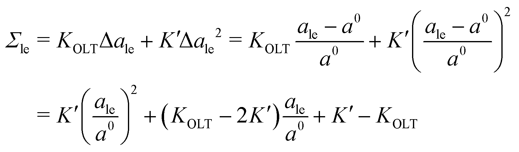
The data for the OLT-deformed bilayers in Fig. 5c display a non-linear tension-area relationship, which are not accounted for by the first-order expressions in eqn (8) and (9). To estimate the linear regime, for which these first-order expressions are reliable, we introduce a second-order correction term and extend the tension-area relationships according to
| |  | (14) |
where the subscript le stands for the upper or lower leaflet ul or ll, with the second-order correction terms proportional to
K′. We use the tension–area relationship in
eqn (14), which is of second order in Δ
ale, to obtain a least squares fit to the data as shown in Fig. S2c (ESI
†). Using the resulting numerical values for the three parameters
a0,
KOLT and
K′, we define the linear regime by the condition |Δ
ale| <
KOLT/10
K′. The data points that satisfy this condition are displayed in
Fig. 5c as filled symbols.
When we use a linear fit for these filled data points, we recover the optimal area per lipid, a0 = 1.219d2 for the symmetric bilayer with 841 lipids in each leaflet as in eqn (5), corresponding to the reference state with tensionless leaflets. The numerical values obtained for the other planar bilayer patches with 600 and 1000 lipids per leaflet are listed in Tables S3 and S4 (ESI†).
2.1.8 Volume per lipid and lateral volume compressibilities.
Next, we introduce the volume per lipid and the lateral volume compressibility to obtain another measure for the leaflet elasticity. First, we define vul and vll to be the volume per lipid in the upper and lower leaflet of the planar bilayer. For a reference state with tensionless leaflets, these two volumes per lipid have the same value which represents the optimal volume per lipid, v0. For bilayers consisting of Nll + Nul = 1682 lipids, this optimal value is| | | v0 = (3.566 ± 0.001)d3 | (15) |
as obtained from Voronoi tessellation (Table S5, ESI†). Inspection of these tables shows that essentially the same optimal volume per lipid is obtained for bilayers with Nll = Nul = 600 and Nll = Nul = 1000.
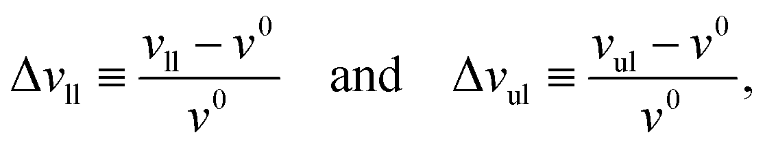
Small deviations of the volumes per lipid, vll and vul, from their optimal volume are described by the volume dilations of the lower and upper leaflet which are defined by
| |  | (16) |
in close analogy to the area dilations in
eqn (7).
To first order in the volume dilations, the elastic response of the two leaflets to the leaflet tensions Σll and Σul is now described by the tension–volume relations
| |  | (17) |
and
| |  | (18) |
which define the lateral volume compressibilities
Bll and
Bul of the lower and upper bilayer leaflets.
The lateral volume compressibilities Bll and Bul as introduced in eqn (17) and (18) describe the elastic response of the volumes per lipid in the two bilayer leaflets to the respective leaflet tensions. These lateral volume compressibilities should be distinguished from the bulk compressibility modulus KV as usually studied in the literature, which represents the elastic response of the bilayer volume to the bulk pressure.60,61 Note that the physical dimension of the lateral volume compressibilities is energy per area whereas the physical dimension of the bulk compressibility modulus is energy per volume.
2.1.9 ELT and OLT deformations versus volume per lipid.
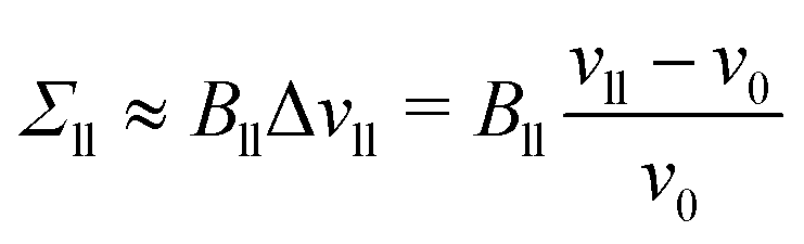
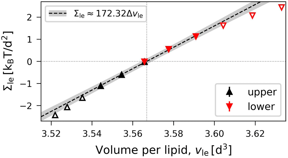
For an ELT deformation of the planar bilayer, the two leaflets experience the same leaflet tension Σul = Σll = Σle. The corresponding lateral volume compressibilities are| | | Bll = Bul ≡ BELT = (156 ± 3)kBT/d2 | (19) |
as follows from the data in Fig. 6. Very similar BELT-values are found for other planar bilayer sizes, see Table S5a (ESI†).
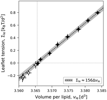 |
| | Fig. 6 Elastic ELT deformations of a symmetric planar bilayer with Nul = Nll = 841. The midplanes of the symmetric ELT states are identical with their symmetry planes: Leaflet tension Σle = Σul = Σll as function of volume per lipid, vle = vul = vll. The dotted vertical line is located at the optimal lipid volume vle = v0 = 3.566d3. The linear fit is based on the filled data symbols. Mean values and standard deviations obtained from 30 statistically independent values of 3 replica simulations. Each of these 30 values is obtained as an average over 100 snapshots, see Methods. Slope and intercept of the linear fit define the values for lateral volume compressibility and optimal volume per lipid viaeqn (17). The linear fit leads to the dashed line, the grey shaded band represents the 95% prediction band. The numerical values of the data are displayed in Table S2 (ESI†). | |
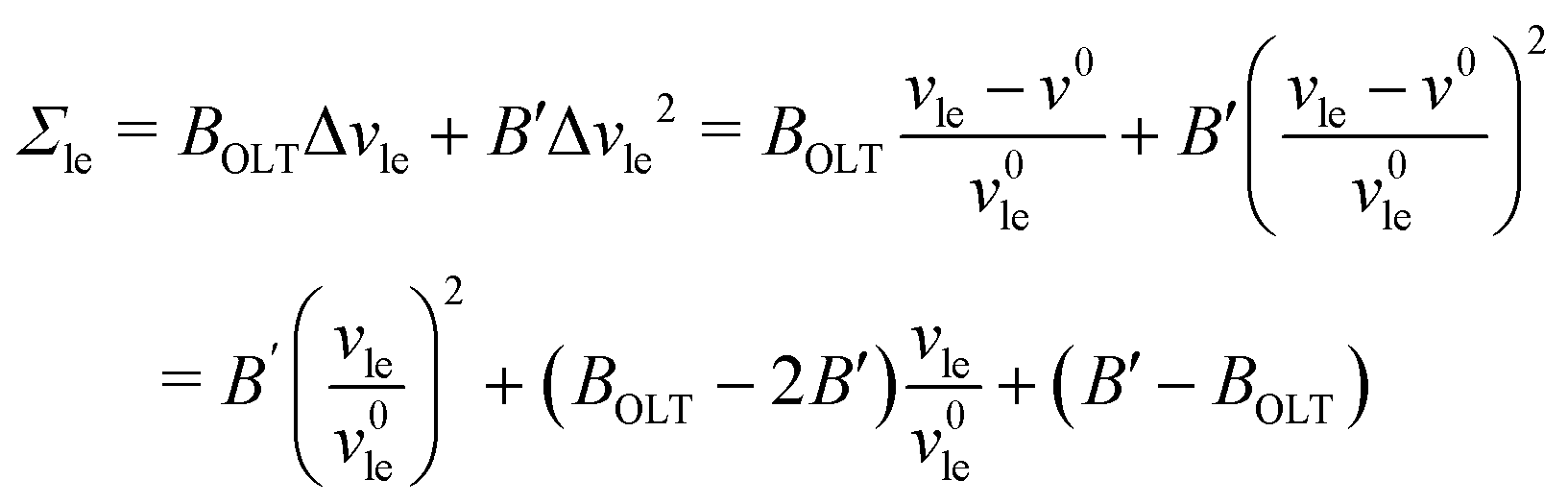
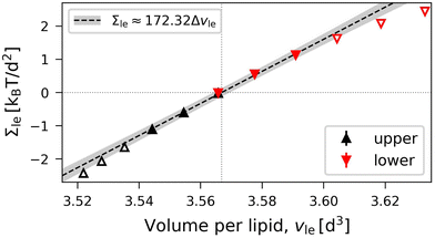
In Fig. 7, OLT deformations of the planar bilayer are displayed in terms of the leaflet tensions as functions of the volume per lipid, vle. As in Fig. 5, the data in Fig. 7 again exhibit slightly non-linear behavior, which can be fitted by the expression
| |  | (20) |
where the subscript ‘le’ stands for ul or ll, corresponding to the upper or lower leaflet, with second-order correction terms proportional to
B′. We use the tension–volume relationship in
eqn (20) to obtain a least squares fit to the data as shown in Fig. S3 (ESI
†). Using the resulting values for
v0,
BOLT, and
B′, we define the linear regime by the condition |Δ
vle| <
B′/(10
BOLT). The data points that satisfy this condition are displayed in
Fig. 7 as filled symbols and lead to the dashed line in
Fig. 7. As a result of this fitting procedure, we obtain the lateral volume compressibility moduli
| | | Bll = Bul ≡ BOLT = (172 ± 4)kBT/d2 | (21) |
for elastic OLT deformations of the bilayers. Note that the lateral compressibility modulus
BOLT is roughly 10% larger than the modulus
BELT for ELT deformations as given by
eqn (19). Very similar
BOLT-values are obtained for other planar bilayer sizes (Table S5b, ESI
†).
 |
| | Fig. 7 OLT deformations of planar bilayer assembled from Nll + Nul = 1682 lipids. The midplanes of the asymmetric OLT states are computed via the VORON protocol: Leaflet tensions Σul and Σll as functions of the volume per lipid, vle. The dotted vertical line is located at the optimal lipid volume v = v0 = 3.566d3. Filled data symbols represent those v-values that belong to the linear regime and fulfill the linearity condition |Δv| < BOLT/(10B′). The linear fit to these filled data is displayed by the dashed line, the grey shaded band represents the 95% prediction band. The numerical values of the data are displayed in Table S3 (ESI†). | |
2.2 Elastic behavior of nanovesicles
2.2.1 Four sizes of nanovesicles.
We study nanovesicles of four different sizes, assembled from Nil + Nol = 1500, 2525, 6312, and 10100 lipids, as shown in Fig. 1. In all four cases, the areas per lipid have different values in the two leaflets. To demonstrate this feature, we first extend the VORON protocol, as described in Section 2.1.3 and illustrated in Fig. 2, from planar bilayers to the case of vesicle bilayers. The VORON protocol for nanovesicles avoids the shortcomings of previous protocols30,34,56 which are based on areas per lipid and necessarily involve some kind of projection onto the curved surfaces of the vesicle bilayers.
2.2.2 VORON protocol for nanovesicles.
The VORON protocol for nanovesicles is based on the computation of the molecular volumes using again three-dimensional Voronoi tessellation, in close analogy to the corresponding procedure for planar bilayers in 2.1.3.
The volumes of the inner and outer leaflets of the vesicle bilayer are denoted by Vil and Vol and are computed by summing up the volumes of all polyhedral cells as in the case of planar bilayers (Fig. 2). The volumes per lipid, vil and vol, of the inner and outer leaflets are then obtained by dividing the leaflet volumes by the number of lipids, Nil and Nol, which leads to
| | 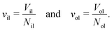 | (22) |
These lipid volumes vary with the leaflet tensions
Σil and
Σol in the inner and outer leaflets. One example for this dependence is shown in
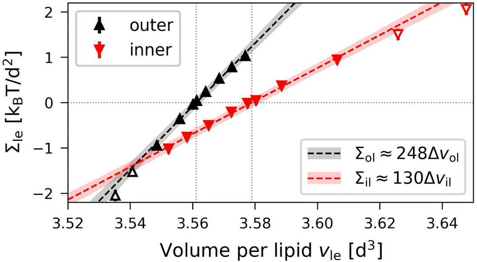
Fig. 8 for a vesicle bilayer assembled from a total number of
Nil +
Nol = 1500 lipids. Inspection of this figure shows that the optimal lipid volumes for the outer and inner leaflet have almost identical but slightly different values as given by
| | | v0il = (3.5790 ± 0.0004)d3 | (23) |
for the inner leaflet and by
| | | v0ol = (3.5612 ± 0.0003)d3 | (24) |
for the outer leaflet of the vesicle, corresponding to the vertical dashed lines in
Fig. 8. Therefore, the optimal lipid volumes for the inner and outer leaflets differ by less than one percent but this small difference is still large compared to the error bars obtained from the statistical data analysis.
 |
| | Fig. 8 Elastic OLT deformations of the smallest nanovesicles with a total number of Nil + Nol = 1500 lipids. The midsurfaces of the vesicle bilayers are computed via the VORON protocol: Leaflet tensions Σle = Σol and Σil of the outer (black data, up-pointing triangles) and inner leaflets (red data, down-pointing triangles) versus volumes per lipid, vle = vil and vle = vol, in the two leaflets of the tensionless bilayers. The two dotted vertical lines are located at the optimal lipid volumes v = v0ol ≃ 3.56d3 and v = v0il ≃ 3.58d3 of the outer and inner leaflet. The filled data symbols close to the optimal lipid volumes are used for linear fits as in eqn (26) and (27), leading to the black and red dashed lines with 95% prediction bands (shaded). The numerical values of the data are in Table S7 (ESI†). | |
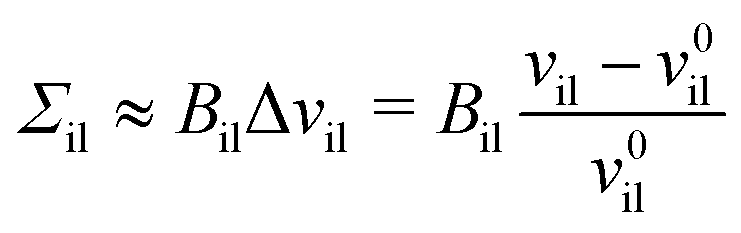
The deviations of the lipid volumes from their optimal values define the volume dilations
| | 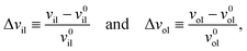 | (25) |
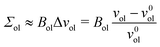
for the inner and outer leaflets. The elastic response of the two leaflets to the leaflet tensions
Σil and
Σol is now described by the tension–volume relations
| | 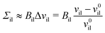 | (26) |
and
| |  | (27) |
to first order in these volume dilations, which define the lateral volume compressibilities
Bil and
Bol. For notational simplicity, we omit the subscript OLT from these moduli.
The OLT data in Fig. 8 exhibit slightly non-linear behavior, similar to the OLT data for planar bilayers in Fig. 7. This nonlinear behavior can again be fitted to the second-order expression in eqn (20), where the subscript ‘le’ now stands for ol and il, corresponding to the outer and inner leaflets. This second-order fit is displayed in Fig. S4 (ESI†).
2.2.3 Vesicle radii from compartment volumes.
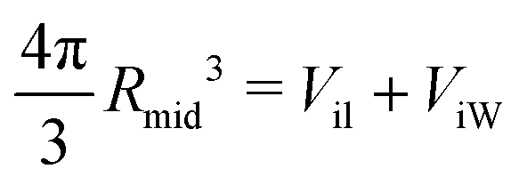
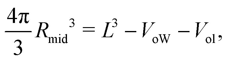
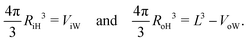
The VORON method can be extended to obtain a simple and unique procedure to compute the midsurface radius Rmid of the vesicle bilayer as well as the radii RiH and RoH of the inner and outer head group layers. The simulation box is a cube with volume L3, in which the closed surface of the vesicle creates two separate water compartments, the inner water compartment with volume ViW and the outer water compartment with volume VoW. The midsurface radius Rmid of the vesicle bilayer can then be computed in two ways, either by using the geometric relation| | 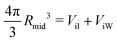 | (28) |
or via the alternative geometric relation| | 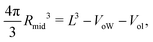 | (29) |
which depends on the volume L3 of the simulation box, the volume VoW of the outer water compartment, and the volume Vol of the outer leaflet. The two relationships in eqn (28) and (29) give identical values for Rmid within the numerical accuracy.
Likewise, we can calculate the radii RiH and RoH of the inner and outer head group layers from the inner and outer water volume using the relationships
| |  | (30) |
The radii
Rmid,
RiH, and
RoH as obtained
viaeqn (28)–(30) are listed in Table S9 (ESI
†) for all four vesicle sizes.
2.2.4 Areas per lipid from volumes per lipid.
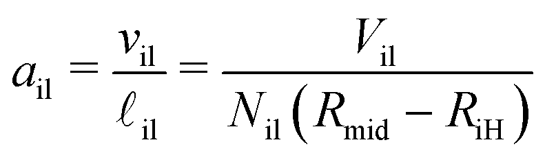
Using the vesicle radii Rmid, RiH, and RoH as determined by the VORON protocol viaeqn (28)–(30), we can also compute the thicknesses of the two leaflets. Indeed, the thicknesses ![[small script l]](https://www.rsc.org/images/entities/char_e146.gif) il and ol of the inner and outer leaflets are given by
il and ol of the inner and outer leaflets are given by| | | il = Rmid − RiH and ol = RoH − Rmid. | (31) |
Finally, dividing the volumes per lipid by the leaflet thicknesses, we can express the areas per lipid in terms of the volumes per lipid and the vesicle radii. This procedure leads to the lipid area| | 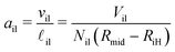 | (32) |
for the inner leaflet, which depends on the inner leaflet volume Vil, the lipid number Nil, and on the two radii Rmid and RiH. Likewise, the area per lipid, aol, in the outer leaflet now becomes| | 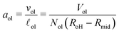 | (33) |
which depends on the outer leaflet volume Vol, the lipid number Nol, and on the two radii RoH and Rmid.
Thus, the VORON protocol for nanovesicles involves two computational steps. First, the midsurfaces of the vesicle bilayers are determined viaeqn (28) and (29), which are then used to decompose the bilayer tensions into its two leaflet contributions. Second, the areas per lipid in the two leaflets are computed viaeqn (32) and (33), which involve the thicknesses of the two leaflets as determined by eqn (31). The VORON protocol for planar bilayers is simpler: it does not involve the second computational step because the areas per lipid follow directly from the base area of the planar bilayers and their computation does not require any decomposition of the bilayers into their leaflets.
2.2.5 Mean curvatures of inner and outer leaflets.
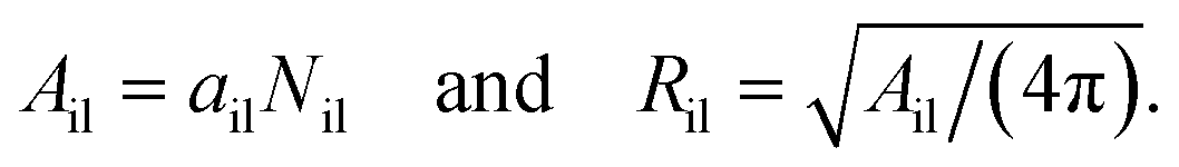
In order to compare the results for nanovesicles of different sizes, it is useful to consider the mean curvatures of the inner and outer leaflets. The inner leaflet contains Nil lipid molecules. Using eqn (32) for the area per lipid, ail, in the inner leaflet, the area Ail and the radius Ril of the inner leaflet's midsurface are computed via| | 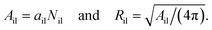 | (34) |
Likewise, using the lipid number Nol and the area per lipid, aol, of the outer leaflet as given by eqn (33), the area Aol and radius Rol of the outer leaflet's midsurface are equal to| | 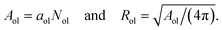 | (35) |
In previous studies based on the CHAIN protocol,30,34 the radii Ril and Rol were obtained using the relations in eqn (S1) and (S2) (ESI†).
The mean curvatures of the inner and outer leaflets are inversely proportional to the midsurface radii Ril and Rol of the two leaflets. Furthermore, in order to display the results for nanovesicles of different sizes, it is useful to take the mean curvature Mil of the inner leaflet to be negative and the mean curvature Mol of the outer leaflet to be positive. Thus, these two mean curvatures are taken to be
| | 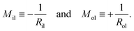 | (36) |
2.2.6 Volumes per lipid for different nanovesicle sizes.
In Fig. 9, the results of the VORON protocol for the optimal lipid volumes v0il and v0ol as well as the lateral volume compressibilities Bil and Bol are plotted as functions of the leaflet mean curvatures Mle for the four different vesicle sizes displayed in Fig. 1. Inspection of Fig. 9a shows that the optimal lipid volumes are essentially constant for the two leaflets and for all four vesicle sizes with v0il ≃ v0ol ≃ (3.56 ± 0.04)d3. The precise numerical values of the two optimal volumes per lipid are given in Table S8 (ESI†).
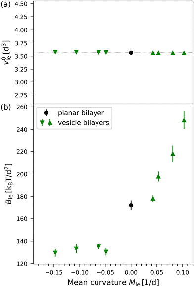 |
| | Fig. 9 Optimal volumes per lipid and lateral volume compressibilities for the four nanovesicles in Fig. 1 as computed by the VORON protocol: (a) optimal volumes per lipid, vle = v0il (down-pointing triangles) for the inner leaflets and vle = v0ol (up-pointing triangles) for the outer leaflets, as functions of mean curvature, which is taken to be negative for the inner leaflets and positive for the outer ones, as in eqn (36); and (b) lateral volume compressibility moduli Bil and Bol for OLT deformations of the inner and outer leaflet versus mean curvature. Green data points represent vesicle leaflets, black data points represent the planar bilayer. Values and errors were obtained by applying least square fits to the data for the leaflet tensions as functions of volume per lipid, as in Fig. 8. The numerical values of the data are in Table S8 (ESI†). | |
On the other hand, the lateral volume compressibility moduli are always significantly higher for the outer leaflet than for the inner one as follows from the data in Fig. 9b. Furthermore, the data in Fig. 9b imply that the inner leaflet volume compressibility changes very little with the mean curvature, whereas the outer leaflet compressibility strongly increases with increasing mean curvature.
2.2.7 Areas per lipid for the smallest nanovesicle.
To illustrate the results obtained by the VORON protocol for the areas per lipid of vesicle bilayers, we first focus on the smallest nanovesicle with a total number of Nil + Nol = 1500 lipids in both leaflets, as shown in Fig. 1b. The corresponding data for the areas per lipid and for the leaflet tensions are displayed in Fig. 10. Panels a and b of Fig. 10 provide the data for the areas per lipid, ail and aol, as well as for the leaflet tensions, Σil and Σol, as functions of the lipid number Nol in the outer leaflet.
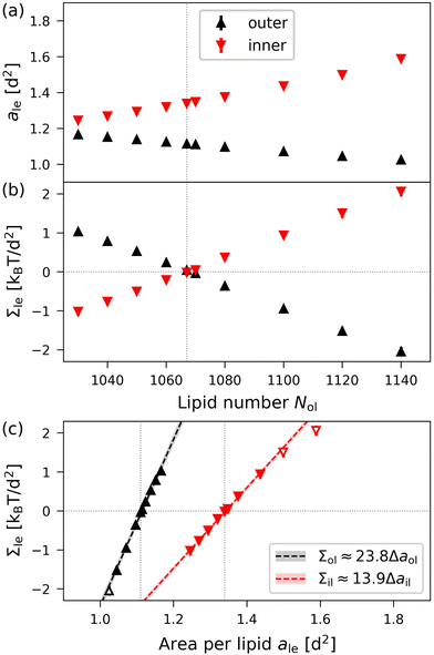 |
| | Fig. 10 Elastic OLT deformations of the smallest nanovesicles with a total number of Nil + Nol = 1500 lipids in both leaflets. (a) and (b) Areas per lipid, ail and aol, as well as leaflet tensions Σil and Σol of the inner and outer leaflets as functions of the lipid number Nol in the outer leaflet. The reference state with tensionless leaflets is described by the vertical dotted lines at Nol = N0ol = 1067; and (c) leaflet tensions Σil and Σol as functions of the lipid areas. The data for the inner leaflet are in red, those for the outer leaflet in black. The midsurfaces of the OLT states as well as the areas per lipid are computed via the VORON protocol, as described in Sections 2.2.3 and 2.2.4. The vertical dotted lines represent the optimal areas per lipid as given by a0ol = 1.114d2 for the outer and a0il = 1.342d2 for the inner leaflet. The numerical values of the data are displayed in Table S7 (ESI†). | |
The areas per lipid are computed using eqn (32) and (33). The leaflet tensions are obtained from the decomposition of the bilayer tension, Σ = Σil + Σol, as described by eqn (48) in the Methods section, where the radius Rmid of the midsurface is determined by eqn (28) and (29). Inspection of Fig. 10b reveals that both leaflet tensions vanish for Nol = N0ol = 1067, which implies N0il = 1500 − N0ol = 433. A combination of the two data sets in Fig. 10a and b provides the leaflet tensions as functions of the areas per lipid as displayed in Fig. 10c. The latter plot shows that the optimal areas per lipid, a0il and a0ol, corresponding to vanishing leaflet tensions, are quite different with a0ol = 1.114d2 for the outer and a0il = 1.342d2 for the inner leaflet.
When the OLT deformations of the smallest nanovesicle Nil + Nol = 1500 lipids are studied by the CHAIN protocol, we obtain the data shown in Fig. S5 (ESI†) as well as Tables S10 and S11 (ESI†). Comparison of Fig. S5 (ESI†) with Fig. 10 shows that the two protocols lead to somewhat different reference states with tensionless leaflets and to different area compressibilities for the two leaflets.
2.2.8 Areas per lipid for different vesicle sizes.
Applying the VORON protocol as described in Sections 2.2.2–2.2.4 to the different sizes of nanovesicles in Fig. 1, we obtain the green data in Fig. 11, which displays the optimal areas per lipid, a0il and a0ol, in Fig. 11a and the area compressibility moduli in Fig. 11b as functions of the mean curvatures Mil and Mol of the inner and outer leaflets. As in eqn (36), the mean curvatures Mil of the inner leaflets are taken to be negative whereas the mean curvatures Mol of the outer leaflets are positive. In Fig. 11, we also include the blue data as obtained from the CHAIN protocol introduced previously30,34 and briefly summarized in Section S1.1 (ESI†).
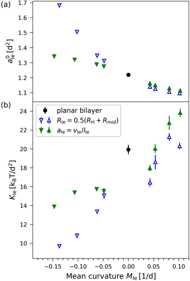 |
| | Fig. 11 Optimal areas per lipid, ale, and area compressibility moduli, Kle, for the four sizes of nanovesicles in Fig. 1, as obtained via the VORON protocol (filled green data points): (a) Optimal areas per lipid, a0il and a0ol, of the inner and outer leaflets versus their mean curvature, which is taken to be positive for the outer and negative for the inner leaflet, as in eqn (36). It follows from these data that, for all nanovesicles, the optimal area per lipid, a0il, in the inner leaflet is larger than the optimal area per lipid, a0ol in the outer leaflet. Futhermore these areas per lipid fulfill the inequalities a0il > a0 > a0ol where a0 (black data point) is the area per lipid of the planar bilayer as in eqn (5); and (b) Area compressibility modulus Kle for OLT deformations of the two leaflets versus their mean curvature. For comparison, another set of data (open blue data points) as obtained from the CHAIN protocol is also included. The black data points for zero mean curvature correspond to the planar bilayer with vanishing mean curvature. Mean values and errors are estimated from least squares fitting of the data for the leaflet tensions as functions of the areas per lipid. The numerical values of the green data are in Table S12 (ESI†), those of the blue data in Table S13a (ESI†). | |
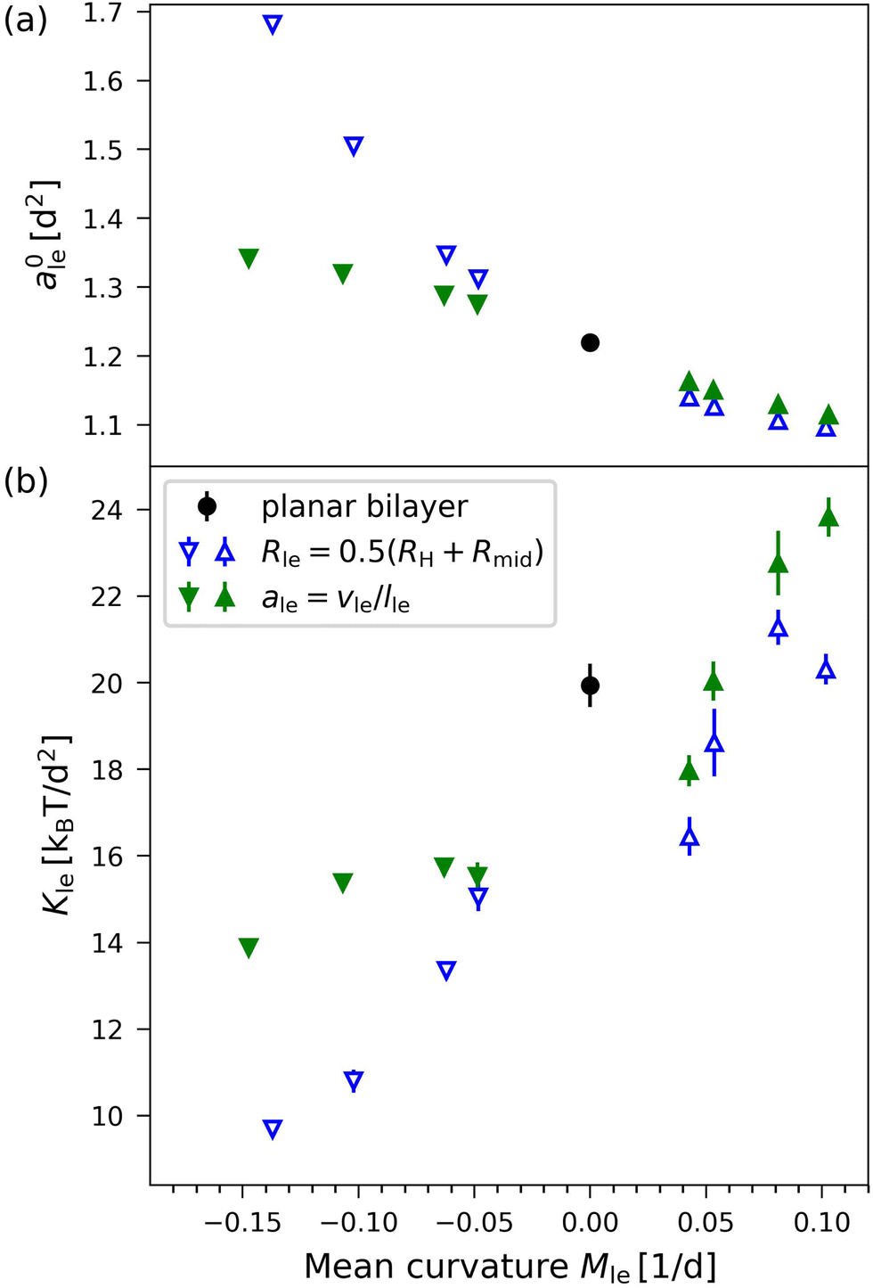
Inspection of Fig. 11a shows that all inner leaflets have an optimal area per lipid, a0il, that is larger than the optimal area per lipid in the planar bilayer, a0ll = a0ul = a0 (black data point), whereas all outer leaflets have an optimal area per lipid, a0ol, that is smaller than a0. As we increase the diameter of the nanovesicle, the areas per lipid in the inner and outer leaflets, a0il and a0ol, should approach the limiting value a0 in the planar bilayer as confirmed by the simulation data in Fig. 11a.
Furthermore, for a certain diameter of the vesicle bilayer, the area per lipid in the inner leaflet is always larger than the area per lipid in the outer leaflet as in Fig. 10a and 11a. Thus, for each nanovesicle, the inner leaflet is more loosely packed compared to the outer leaflet. This difference in molecular packing is consistent with the intuitive view that lipids with two hydrocarbon chains prefer to reside in a weakly rather than in a strongly curved surface. Therefore, when these lipids are forced to pack into the more highly curved inner leaflet, they experience an increased “geometric frustration” which leads to a looser molecular packing and to an increased area per lipid. In contrast, the computational procedure used in ref. 56 leads to areas per lipid in the outer leaflet that are larger than the areas per lipid in the inner leaflets (Section S1.2, Fig. S6 and Table S10, ESI†).
2.2.9 Area compressibilities of vesicle leaflets.
We now consider elastic deformations of the reference states of the nanovesicles which lead to deviations of the areas per lipid from their optimal values. We focus on elastic OLT deformations, in which we start from a reference state with tensionless leaflets and first reshuffle lipids between the two leaflets for constant total lipid number Nil + Nol. In a second step, we then adjust the vesicle volume to obtain a bilayer with vanishing bilayer tension, Σ = Σil + Σol = 0. In close analogy to the planar bilayer case, we define the area dilations| |  | (37) |
and| |  | (38) |
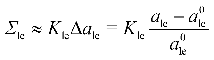
To leading order in these area dilations, the leaflet tensions Σle with le = il or le = ol behave as| | 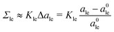 | (39) |
during elastic OLT deformations where Kle represents the area compressibility modulus of the inner or outer leaflet. For notational simplicity, we omit the subscript OLT from the modulus Kle, but all area compressibilities for nanovesicles as described here and below are obtained for OLT deformations.
The data for the area compressibilities Kil and Kol as obtained via the VORON protocol are displayed by the filled green data symbols in Fig. 11b as a function of the mean curvature of the two leaflets, where we again take the inner and outer leaflets to have negative and positive mean curvature, respectively, as in eqn (36). In Fig. 11b, we also include the open blue data as obtained by computing the midsurfaces of the two leaflets from the CHAIN protocol as discussed in Section S1.1 (ESI†). For both data sets in Fig. 11b, the area compressibility modulus increases monotonically with increasing mean curvature. Therefore, we conclude that the area compressibilities of the two leaflets satisfy
| | | Kil < Kol (elastic OLT deformations) | (40) |
which implies that the inner leaflet is more compressible than the outer one.
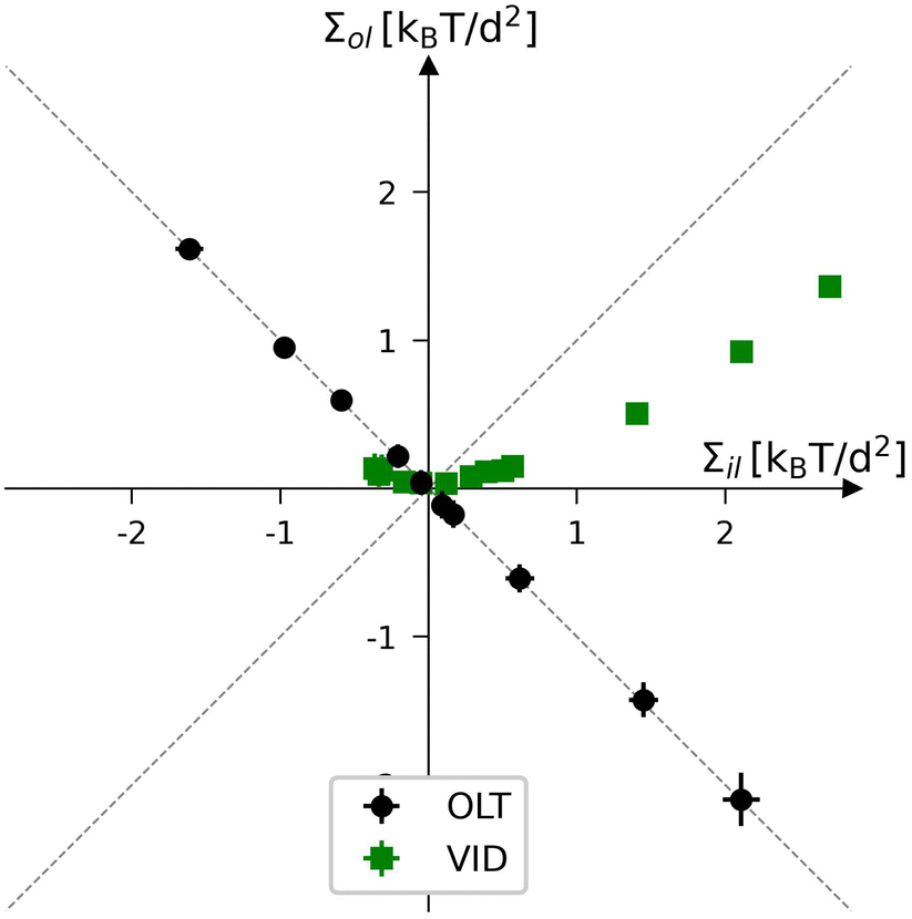
2.2.10 Leaflet tension space for nanovesicles.
For nanovesicles, elastic OLT deformations can be studied in close analogy to the OLT deformations of planar bilayers. These deformations correspond to the black data in Fig. 12 which displays the leaflet tension space for vesicle bilayers with a total number of Nil + Nol = 2525 lipids in both leaflets. The reference state with tensionless leaflets is obtained for Nil = 840 and Nol = 1685. Each of the black data points in Fig. 12 involves the reshuffling of a certain number of lipids from one leaflet to the other and changing the vesicle volume to reach a vesicle bilayer with vanishing bilayer tension Σ = Σil + Σol = 0.
 |
| | Fig. 12 Leaflet tension space for the closed bilayers of nanovesicles with a total number of Nil + Nol = 2525 lipids in both leaflets. The two coordinates are the leaflet tensions Σil and Σol in the inner and outer leaflets. The midsurfaces of the vesicle bilayers are determined via the VORON protocol. Negative and positive leaflet tensions describe compressed and stretched leaflets. The reference state with tensionless leaflets, corresponding to Σil = Σol = 0, is obtained for a vesicle bilayer with Nil = 840 lipids in the inner leaflet and Nol = 1685 lipids in the outer one. The black data correspond to elastic OLT deformations obtained from the reference state by reshuffling lipids from one leaflet to the other and adjusting the vesicle volume to obtain tensionless bilayers with Σ = Σil + Σol = 0. The green data represent the elastic deformations arising from changes in vesicle volume, corresponding to vesicle inflation or deflation (VID). The numerical values of the VID data are in Table S14 (ESI†). | |
To generate the green data for vesicle inflation or deflation (VID) in Fig. 12, we start again from the reference state with Σil = Σol = 0 but now change the vesicle volume in order to increase or decrease the bilayer tension, thereby mimicking the experimental procedure of osmotic inflation or deflation. Note that the green data do not follow the main diagonal, in contrast to the equal leaflet tension (ELT) data in Fig. 3. Therefore, during a VID step, both leaflet tensions are changed by different amounts. In order to obtain a vesicle bilayer with equal leaflet tensions, Σil = Σol, we have to add a second step, in which lipids are again reshuffled between the leaflets. However, compared to the OLT deformations, the lipid reshuffling has to be iterated several times because we need to change both leaflet tensions in different ways. Thus, during each of these iterative steps, we vary the lipid numbers, Nil and Nol, in the two leaflets, determine the corresponding midsurface of the vesicle bilayer, and compute the two leaflet tensions from the decomposition of the stress profile, a somewhat tedious and time-consuming procedure.
3 Summary and outlook
In summary, we studied the elastic properties of lipid bilayers, both for planar and for spherical geometries as displayed in Fig. 1. For planar geometry, we primarily studied bilayers with a total number of 1682 lipids in both leaflets. To compute the leaflet tensions Σll and Σul in the lower and upper leaflets of asymmetric bilayers, we introduced a new computational method, called VORON, to determine the midsurfaces of these bilayers (Section 2.1.4). This method is based on computing the molecular volumes of lipid and water molecules via Voronoi tessellation (Fig. 2).
We then used the two leaflet tensions Σll and Σul in the lower and upper leaflets to define a two-dimensional parameter space for such bilayers (Fig. 3). We focussed on two types of elastic deformations characterized by equal leaflet tensions (ELT) with Σul = Σll and by opposite leaflet tensions (OLT) with Σul = −Σll. We then determined the area compressibility moduli both for ELT and for OLT deformations. The data for ELT and OLT deformations are displayed in Fig. 4 and 5, the analysis of these data leads to the numerical values for the area compressibility moduli KELT and KOLT in eqn (12) and (13). Our data clearly show that KELT and KOLT have different numerical values.
Next, we characterized the reference states of planar bilayers with tensionless leaflets by their optimal volumes per lipid and introduced lateral volume compressibilities, BELT and BOLT, to describe the response of the lipid volume to ELT and OLT deformations. The numerical value of the optimal volume per lipid, vle, is given by eqn (15) and the lateral volume compressibilities BELT and BOLT ≠ BELT by eqn (19) and (21).
Planar bilayers have zero mean curvature. To address the curvature dependence of the elastic behavior, we studied four different sizes of nanovesicles as shown in Fig. 1b–e. The extension of the VORON protocol to nanovesicles is described in Sections 2.2.2–2.2.4. As for planar bilayers, this protocol is based on the volumes of the individual molecular groups which are computed by Voronoi tessellation. As a result of this protocol, we obtained the optimal volumes per lipid, which characterize the reference states with tensionless leaflets, as well as the lateral volume compressibilities.
The optimal volumes per lipid, v0il for the inner and v0ol for the outer leaflets, are displayed in Fig. 9a for the different vesicle sizes studied here. Inspection of this figure reveals that the optimal lipid volumes are essentially independent of vesicle size and have practically the same value in both leaflets, see also the optimal volumes per lipid for the smallest nanovesicle as given by eqn (23) and (24). The elastic response of the lipid volume to the leaflet tensions defines the lateral volume compressibilities Bil and Bol of the inner and outer leaflets, see eqn (26) and (27). These compressibilities are plotted in Fig. 9b for the different vesicle sizes and in the inset of Fig. 8 for the smallest nanovesicle. The data in Fig. 9b imply that Bil and Bol have rather different values for all sizes of the nanovesicles. More precisely, these data reveal that the lipid volume in the inner leaflet of a nanovesicle is always more compressible than in the outer leaflet.
Using the VORON protocol, the areas per lipid can also be computed in the two leaflets of vesicle bilayers, using the volumes of different subcompartments as described in Section 2.2.4. For the smallest nanovesicles, this procedure leads to areas per lipid as displayed in Fig. 10 as functions of the lipid number in the outer leaflet. Inspection of this figure reveals that the area per lipid in the outer leaflet is always smaller than the area per lipid in the inner leaflet, which implies that the lipids are more densely packed in the outer leaflet. The same difference in the packing densities is also observed for larger nanovesicles. This property is demonstrated in Fig. 11a for the optimal areas per lipid, a0il in the inner leaflets and a0ol < a0il in the outer leaflets. The area compressibilities obtained from the VORON protocol are shown by the green data symbols in Fig. 11b. The latter data imply that the area compressibility modulus of the outer leaflet is larger than the modulus of the inner leaflet, that is, that the inner leaflet is more compressible than the outer leaflet.
The VORON protocol developed here will be useful for a variety of more complex bilayer systems. First of all, this protocol can be extended to bilayers with several lipid components. These systems involve additional compositional variables and may exhibit two-phase coexistence regions which lead to different domains within the bilayers. One particularly interesting system are multicomponent bilayers with one lipid species that undergoes frequent flip–flops on the time scale of the simulations. For planar bilayers, the results of two previous studies33,62 led to different conclusions about the time-dependent relaxation of the leaflet tensions, and it would be rather interesting to extend these studies to nanovesicles.
Finally, the VORON protocol may also be applied to non-spherical shapes of nanovesicles. One challenge to address in future simulation studies is the optimal volume per lipid for such more complex shapes of the nanovesicles. Based on our result that the volume per lipid is practically independent of the size and mean curvature of the vesicles (Fig. 9a), we expect that essentially the same volume per lipid applies to all vesicle shapes as well.
4 Methods
4.1 Dissipative particle dynamics (DPD)
DPD is a coarse-grained molecular dynamics simulation technique for which the molecular model is built up from soft beads with short-range interactions. Compared to other simulation methods, the DPD approach has several advantages as described in our recent review.63 Our systems are built up from water (W) beads representing, on average, three water molecules and from lipid molecules with two chains, each of which consists of six hydrophobic chain (C) beads31 as shown in Fig. 13. The lipid head group connecting the two chains is represented by three hydrophilic head (H) beads. All beads have the same diameter d and the same mass mbe.
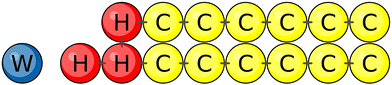 |
| | Fig. 13 Different types of beads used for the coarse-grained lipid–water model studied here: water (W) bead (blue) representing three water molecules. A lipid molecule consists of three head group (H) beads (red) and two linear hydrocarbon chains, each of which contains six chain (C) beads (yellow). Bonded interactions are indicated by short black tics connecting two beads. | |
The bulk water density has the standard DPD value ρW = 3/d3 to reproduce the compressibility of bulk water at room temperature T = 298 K.64 To suppress finite size effects as observed, e.g., in ref. 65, the water bead density away from the bilayer is always taken to be equal to ρW = 3/d3. We use dimensionless quantities defined in units of the bead diameter d, the bead mass mbe, and the thermal energy kBT, where kB is the Boltzmann constant.
4.2 Interaction forces between beads
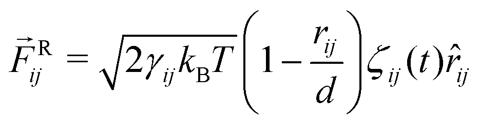
The total force acting between two beads consists of three terms:66,67 the conservative force ![[F with combining right harpoon above (vector)]](https://www.rsc.org/images/entities/i_char_0046_20d1.gif) C, the dissipative force D, and the random force R. When the forces act between two beads i and j with position vectors
C, the dissipative force D, and the random force R. When the forces act between two beads i and j with position vectors ![[r with combining right harpoon above (vector)]](https://www.rsc.org/images/entities/i_char_0072_20d1.gif) i and j, they depend on the quantities
i and j, they depend on the quantities| |  | (41) |
where ![[r with combining circumflex]](https://www.rsc.org/images/entities/i_char_0072_0302.gif) ij is the unit vector pointing from j to i. The conservative force Cij acting between i and j is
ij is the unit vector pointing from j to i. The conservative force Cij acting between i and j is| | 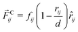 | (42) |
for 0 < rij ≤ d and vanishes for rij > d. The force parameters fij are displayed in Table 1 and have the same values as in previous studies.30,31
Table 1 Conservative and dissipative force parameters, fij and γij
|
f
ij
|
H |
C |
W |
| H |
30 |
50 |
30 |
| C |
|
10 |
75 |
| W |
|
|
25 |
|
γ
ij
|
H |
C |
W |
| H |
4.5 |
9.0 |
4.5 |
| C |
|
4.5 |
20.0 |
| W |
|
|
4.5 |
The dissipative force Dij is given by
| |  | (43) |
with the dissipative force parameter
γij as in
Table 1 and the velocity difference vector
![[v with combining right harpoon above (vector)]](https://www.rsc.org/images/entities/i_char_0076_20d1.gif) ij
ij ≡
i −
j. Finally, the random force
Rij represents thermal noice acting on the two beads
i and
j and is taken to be
| |  | (44) |
where
ζij(
t) represents Gaussian white noise.
The force parameters fij and γij in Table 1 are chosen to mimic hydrophobic interactions. For example, repulsive and dissipative forces between a water bead and a chain bead are significantly stronger than those between a water bead and a headgroup bead, leading to bilayer or micelle formation in a lipid–water mixture.
Bonded interaction potentials between the H and C beads do not depend on the bead type and are taken to have the harmonic form
| | | Ubond(r) = k(r − r0)2 | (45) |
for the distance
r between the bonded beads with the spring constant
k = 64
kBT/
d2 and the equilibrium distance
r0 = 0.5
d. In addition, in the lipid chains, two neighboring bonds, which connect three C beads and form the angle
Θ, experience the bending potential
| | | Ubend(Θ) = kΘ(1 − cos(Θ − Θ0)) | (46) |
with the bending constant
kΘ = 15
kBT and the optimal bond–bond angle
Θ0 = π = 180°.
4.3 System preparation
Planar bilayers.
We assembled and simulated three different sizes of planar bilayers, which contained a total number of Nll + Nul = 1200, 1682, and 2000 lipids in the lower and upper leaflets. In the main text, we focus on planar bilayers with Nll + Nul = 1682 but additional results on the other two sizes are provided in the ESI.† We observed no flip–flops, i.e., each lipid remained in its initial leaflet throughout the simulations.
Nanovesicles.
We assembled and studied nanovesicles of four different sizes, with Nil and Nol lipids in the inner and outer leaflets. The largest vesicle with Nil + Nol = 10100 was assembled with the initial radius Rini = 22.1d, corresponding to the equilibrated value obtained previously.30 Here, we extended these previous simulations and added three smaller nanovesicles with a total lipid number of Nil + Nol = 6312, 2525, and 1500 lipids. For each value of Nil + Nol, we simulated seven to nine vesicles with different lipid distributions in the two leaflets (Table S15, ESI†).
To assemble the nanovesicles, the inner leaflet was initially placed on a spherical shell between Rini − 2.79d and Rini, and the outer leaflet on a shell between Rini and Rini + 2.194d. The values for the leaflet thicknesses (2.79d and 2.194d) were extracted from the data for the reference system in ref. 30. Water beads inside the vesicle were initially placed inside a sphere of radius Rini − 2.79d, and the external water beads filled the volume outside a sphere of radius Rini + 2.105d.
The initial vesicle radii Rini, the total number of water beads, NoW, in the outer water compartment, and the linear dimensions L of the cubic box sizes are listed in Table S15 (ESI†). For each value of the total lipid numbers, Nil + Nol, the number of water beads outside the vesicle, NoW, was kept fixed, while the number of internal waters, NiW, was adjusted to reach the tensionless bilayer state. These tensionless states can be reached in an iterative manner starting from an educated guess for NiW.
4.4 Simulation protocols
The initial lipid–water systems were set up using packmol68 and subsequently translated into LAMPPS-readable format with moltemplate.69 In order to determine the reference state and the OLT deformations of the planar bilayers, which are characterized by vanishing bilayer tension, we used the semi-isotropic NPT ensemble to equilibrate the bilayers for 125000 timesteps or about 1.25 μs. For ELT deformations, the barostat was applied only along the z-direction. Each nanovesicle, consisting of Nil lipids in the inner leaflet, Nol lipids in the outer leaflets and NiW water beads within the vesicle interior, was also equilibrated for 125000 timesteps ≈1.25 μs, now in the isotropic NPT-ensemble. Three replicas of these equilibrated systems were run independently for another 1.25 μs in the NVT-ensemble, followed by a 5 μs production run in NVT. The replicas started from the same initial bead positions and bead velocities, but with different random number generator seeds.
4.5 Bead densities and statistical analysis
Distributions and densities of the head, chain, and water beads were obtained using the LAMMPS built-in tool. Leaflet volumes were calculated as the sum of volumes of Voronoi cells assigned to specific bead types divided by the number of lipids in each leaflet, see eqn (2) for planar bilayers and eqn (22) for nanovesicles. The Voronoi tessellation is implemented within the LAMMPS package,57 using the Voro++ library.58
All calculated values (pressure tensor components, densities, volumes) were sampled by averaging over 500 frames with 100 time steps in between. Such sampling was performed every 50000 frames, to obtain 10 values for each simulation, and 30 for each system. The bin width in the radial coordinate was 0.25d. All integration operations were made using the trapezoid method.
4.6 Stress profiles and leaflet tensions
Planar bilayers.
For a planar bilayer, the normal and tangential components of the pressure tensor, PN and PT, depend only on the Cartesian coordinate z perpendicular to the bilayer. As a consequence, the stress profile across the bilayer depends on z and is given by s(z) = PN(z) − PT(z).29,70–72 The stress profile was computed by using the LAMMPS implementation of the pressure tensor.73 The bilayer tension Σ of the planar bilayer was obtained by integrating the stress profile s(z) over z.
The decomposition of the bilayer tension Σ into the two leaflet tensions Σll and Σul was achieved by the definition of an approriate midplane based on the VORON protocol, see Sections 2.1.3 and 2.1.4, which leads to31,34
| |  | (47) |
The integration limits
zmid − 7
d and
zmid + 7
d ensure that each integration covers the whole leaflet but, at the same time, cuts off the fluctuations in the stress profile arising from thermally-excited density fluctuations and bilayer undulations.
Spherical nanovesicles.
Because of the spherical symmetry, the normal and tangential components of the pressure tensor now depend on the radial coordinate r, and the stress profile across the bilayer is given by s(r) = PN(r) − PT(r).30,72,73 The bilayer tension Σ is obtained by integrating the stress profile s(r) over r, and the two leaflet tensions Σil and Σol of the inner and outer leaflet are obtained via| |  | (48) |
The radius Rmid of the bilayer's midsurface was determined by the VORON protocol as explained in Sections 2.2.2–2.2.4. In Fig. 11, the results of the VORON protocol are compared with the results of the CHAIN protocol; in Fig. S6 (ESI†), these results are also compared with an alternative procedure56 based on the headgroup layers.
Conflicts of interest
There are no conflicts to declare.
Acknowledgements
This research was conducted within the Max Planck School Matter to Life supported by the German Federal Ministry of Education and Research (BMBF) in collaboration with the Max Planck Society and the Max Planck Institute of Colloids and Interfaces. Open Access funding provided by the Max Planck Society.
Notes and references
- E. Gorter and F. Grendel, J. Exp. Med., 1925, 41, 439–443 CrossRef CAS PubMed.
- J. D. Robertson, Biochem. Soc. Symp., 1959, 16, 3–43 CAS.
- J. D. Robertson, Prog. Biophys. Biophys. Chem., 1960, 10, 343–418 CrossRef CAS.
- A. Bangham and R. Horne, J. Mol. Biol., 1964, 8, 660–668 CrossRef CAS.
- R. Lipowsky, Nature, 1991, 349, 475–481 CrossRef CAS PubMed.
- in Physics of Biological Membranes, ed. P. Bassereau and P. Sens, Springer Nature, 2018 Search PubMed.
- in The Giant Vesicle Book, ed. R. Dimova and C. Marques, Taylor & Francis, 2019 Search PubMed.
- R. P. Rand and A. C. Burton, Biophys. J., 1964, 4, 115–135 CrossRef CAS PubMed.
- R. M. Hochmuth, J. Biomech., 2000, 33, 15–22 CrossRef CAS PubMed.
- E. Evans and A. Yeung, Biophys. J., 1989, 56, 151–160 CrossRef CAS PubMed.
- J.-Y. Tinevez, U. Schulze, G. Salbreux, J. Roensch, J.-F. Joanny and E. Paluch, Proc. Natl. Acad. Sci. U. S. A., 2009, 106, 18581–18586 CrossRef CAS PubMed.
- E. Evans and D. Needham, J. Phys. Chem., 1987, 91, 4219–4228 CrossRef CAS.
- W. Rawicz, K. C. Olbrich, T. McIntosh, D. Needham and E. Evans, Biophys. J., 2000, 79, 328–339 CrossRef CAS PubMed.
- V. Heinrich and R. E. Waugh, Ann. Biomed. Eng., 1006, 24, 595–605 CrossRef PubMed.
- D. Cuvelier, I. Derenyi, P. Bassereau and P. Nassoy, Biophys. J., 2005, 88, 2714–2726 CrossRef CAS PubMed.
- B. Sorre, A. Callan-Jones, J. Manzi, B. Goud, J. Prost, P. Bassereau and A. Roux, Proc. Natl. Acad. Sci. U. S. A., 2012, 109, 173–178 CrossRef CAS PubMed.
- D. Roy, J. Steinkühler, Z. Zhao, R. Lipowsky and R. Dimova, Nano Lett., 2020, 20, 3185–3191 CrossRef CAS PubMed.
- J. Dai and M. Sheetz, Biophys. J., 1999, 77, 3363–3370 CrossRef CAS PubMed.
- B. Pontes, P. Monzo and N. C. Gauthier, Semin. Cell Dev. Biol., 2017, 71, 30–41 CrossRef CAS PubMed.
- E. Sitarska and A. Diz-Muñoz, Curr. Opin. Cell Biol., 2020, 66, 11–18 CrossRef CAS PubMed.
- H. Deuling and W. Helfrich, J. Phys., 1976, 37, 1335–1345 CrossRef CAS.
- U. Seifert, K. Berndl and R. Lipowsky, Phys. Rev. A: At., Mol., Opt. Phys., 1991, 44, 1182–1202 CrossRef CAS PubMed.
- R. Lipowsky, Adv. Colloid Interface Sci., 2014, 208, 14–24 CrossRef CAS PubMed.
- U. Seifert and R. Lipowsky, Phys. Rev. A: At., Mol., Opt. Phys., 1990, 42, 4768–4771 CrossRef CAS PubMed.
- R.-M. Servuss and W. Helfrich, J. Phys., 1989, 50, 809–827 CrossRef CAS.
- T. Gruhn, T. Franke, R. Dimova and R. Lipowsky, Langmuir, 2007, 23, 5423–5429 CrossRef CAS PubMed.
- E. Evans, H. Bowman, A. Leung, D. Needham and D. Tirrell, Science, 1996, 273, 933–935 CrossRef CAS PubMed.
- M. Karlsson, M. Davidson, R. Karlsson, A. Karlsson, H. Bergenholtz, Z. Konkoli, A. Jesorka, T. Lobovkina, J. Hurtig, M. Voinova and O. Orwar, Annu. Rev. Phys. Chem., 2004, 55, 613–649 CrossRef CAS PubMed.
- R. Goetz and R. Lipowsky, J. Chem. Phys., 1998, 108, 7397–7409 CrossRef CAS.
- R. Ghosh, V. Satarifard, A. Grafmüller and R. Lipowsky, Nano Lett., 2019, 19, 7703–7711 CrossRef CAS PubMed.
- B. Rózycki and R. Lipowsky, J. Chem. Phys., 2015, 142, 054101 CrossRef PubMed.
- A. Sreekumari and R. Lipowsky, J. Chem. Phys., 2018, 149, 084901 CrossRef PubMed.
- M. Miettinen and R. Lipowsky, Nano Lett., 2019, 19, 5011–5016 CrossRef CAS PubMed.
- A. Sreekumari and R. Lipowsky, Soft Matter, 2022, 18, 6066–6078 RSC.
- P. J. Beltramo, R. V. Hooghten and J. Vermant, Soft Matter, 2016, 12, 4324–4331 RSC.
- I. Mey, C. Steinem and A. Janshoff, J. Mater. Chem., 2012, 22, 19348–19356 RSC.
- A. Jahn, S. M. Stavis, J. S. Hong, W. N. Vreeland, D. L. DeVoe and M. Gaitan, ACS Nano, 2010, 4, 2077–2087 CrossRef CAS PubMed.
- B. S. Pattni, V. V. Chupin and V. P. Torchilin, Chem. Rev., 2015, 115, 10938–10966 CrossRef CAS PubMed.
- G. Cevc and G. Blume, Biochim. Biophys. Acta, 1992, 1104, 226–232 CrossRef CAS PubMed.
- E. Touitou, N. Dayan, L. Bergelson, B. Godin and M. Eliaz, J. Controlled Release, 2000, 65, 403–418 CrossRef CAS PubMed.
- B. Bhasin and V. Y. Londhe, IJPSR, 2018, 9(6), 2175–2184 CAS.
- F. Lai, C. Caddeo, M. L. Manca, M. Manconi, C. Sinico and A. M. Fadda, Int. J. Pharm., 2020, 583, 119398 CrossRef CAS PubMed.
- T. Limongi, F. Susa, M. Marini, M. Allione, B. Torre, R. Pisano and E. D. Fabrizio, J. Nanomater., 2021, 11, 3391–3429 CrossRef CAS PubMed.
- S. Rai, V. Pandey and G. Rai, Nano Rev. Exp., 2017, 8, 1325708–1325720 CrossRef PubMed.
- G. Damiani, A. Pacifico, D. M. Linder, P. D. M. Pigatto, R. Conic, A. Grada and N. L. Bragazzi, Dermatol. Ther., 2019, 32, e13113 Search PubMed.
- J. A. Kulkarni, D. Witzigmann, S. Chen, P. R. Cullis and R. V. D. Meel, Acc. Chem. Res., 2019, 52, 2435–2444 CrossRef CAS PubMed.
- Y. Suzuki and H. Ishihara, Drug Metab. Pharmacokinet., 2021, 41, 100424–100431 CrossRef CAS PubMed.
- S. Pengnam, S. Plianwong, B. E. Yingyongnarongkul, P. Patrojanasophon and P. Opanasopit, Drug Metab. Pharmacokinet., 2022, 42, 100425 CrossRef CAS PubMed.
- M. Chen, X. Hu and S. Liu, Macromol. Chem. Phys., 2022, 223, 2100443 CrossRef CAS.
- S. Ramachandran, S. R. Satapathy and T. Dutta, J. Pharm. Med., 2022, 36, 11–20 CrossRef CAS PubMed.
- E. Woith, G. Fuhrmann and M. F. Melzig, Int. J. Mol. Sci., 2019, 20, 5695 CrossRef CAS PubMed.
- L. Barile and G. Vassalli, Pharmacol. Therapeut., 2017, 174, 63–78 CrossRef CAS PubMed.
- I. Jalaludin, D. M. Lubman and J. Kim, Mass Spectrosc. Rev., 2021, e21749 Search PubMed.
- I. K. Herrmann, M. J. A. Wood and G. Fuhrmann, Nat. Nanotechnol., 2021, 16, 748–759 CrossRef CAS PubMed.
- L. van der Koog, T. B. Gandek and A. Nagelkerke, Adv. Healthcare Mater., 2022, 11, 2100639 CrossRef CAS PubMed.
- H. J. Risselada and S. J. Marrink, Phys. Chem. Chem. Phys., 2009, 11, 2056–2067 RSC.
- A. P. Thompson, H. M. Aktulga, R. Berger, D. S. Bolintineanu, W. M. Brown, P. S. Crozier, P. J. in 't Veld, A. Kohlmeyer, S. G. Moore, T. D. Nguyen, R. Shan, M. J. Stevens, J. Tranchida, C. Trott and S. J. Plimpton, Comput. Phys. Comm., 2022, 271, 108171 CrossRef CAS.
- C. H. Rycroft, CHAOS, 2009, 19, 041111 CrossRef PubMed.
-
V. A. Parsegian and R. P. Rand, The Structure and Dynamics of Membranes, Elsevier, Amsterdam, 1995, vol. 1, pp. 643–690 Search PubMed.
-
G. Cevc and D. Marsh, Phospholipid bilayers: physical principles and models, Wiley, New York, 1987 Search PubMed.
- M. M. Terzi, M. Deserno and J. F. Nagle, Soft Matter, 2019, 15, 9085–9092 RSC.
- A. Hossein and M. Deserno, Biophys. J., 2020, 118, 624–642 CrossRef CAS PubMed.
- R. Lipowsky, R. Ghosh, V. Satarifard, A. Sreekumari, M. Zamaletdinov, B. Rózycki, M. Miettinen and A. Grafmüller, Biomolecules, 2023, 13, 926 CrossRef CAS PubMed.
- R. D. Groot and P. B. Warren, J. Chem. Phys., 1997, 107, 4423–4435 CrossRef CAS.
- L. Gao, J. Shillcock and R. Lipowsky, J. Chem. Phys., 2007, 126, 015101 CrossRef PubMed.
- R. D. Groot and T. J. Madden, J. Chem. Phys., 1998, 108, 8713–8724 CrossRef CAS.
- J. C. Shillcock and R. Lipowsky, J. Chem. Phys., 2002, 117, 5048–5061 CrossRef CAS.
- L. Martnez, R. Andrade, E. G. Birgin and J. M. Martnez, J. Comput. Chem., 2009, 30, 2157–2164 CrossRef PubMed.
- A. I. Jewett, D. Stelter, J. Lambert, S. M. Saladi, O. M. Roscioni, M. Ricci, L. Autin, M. Maritan, S. M. Bashusqeh, T. Keyes, R. T. Dame, J.-E. Shea, G. J. Jensen and D. S. Goodsell, J. Mol. Biol., 2021, 433, 166841 CrossRef CAS PubMed.
- J. H. Irving and J. G. Kirkwood, J. Chem. Phys., 1950, 18, 817–829 CrossRef CAS.
- P. Schofield and J. R. Henderson, Proc. R. Soc. London, Ser. A, 1982, 379, 231–246 Search PubMed.
-
J. Rowlinson and B. Widom, Molecular Theory of Capillarity, Oxford University Press, Oxford, 1989 Search PubMed.
- T. Nakamura, S. Kawamoto and W. Shinoda, Comput. Phys. Commun., 2015, 190, 120–128 CrossRef CAS.
Footnote |
| † Electronic supplementary information (ESI) available: Section S1; Fig. S1–S6; Tables S1–S6 for planar bilayers; Tables S7–S15 for nanovesicles. See DOI: https://doi.org/10.1039/d3sm00351e |
|
| This journal is © The Royal Society of Chemistry 2023 |
Click here to see how this site uses Cookies. View our privacy policy here. 
 Open Access Article
 This Open Access Article is licensed under a
  *abc and
Reinhard
Lipowsky
*abc and
Reinhard
Lipowsky
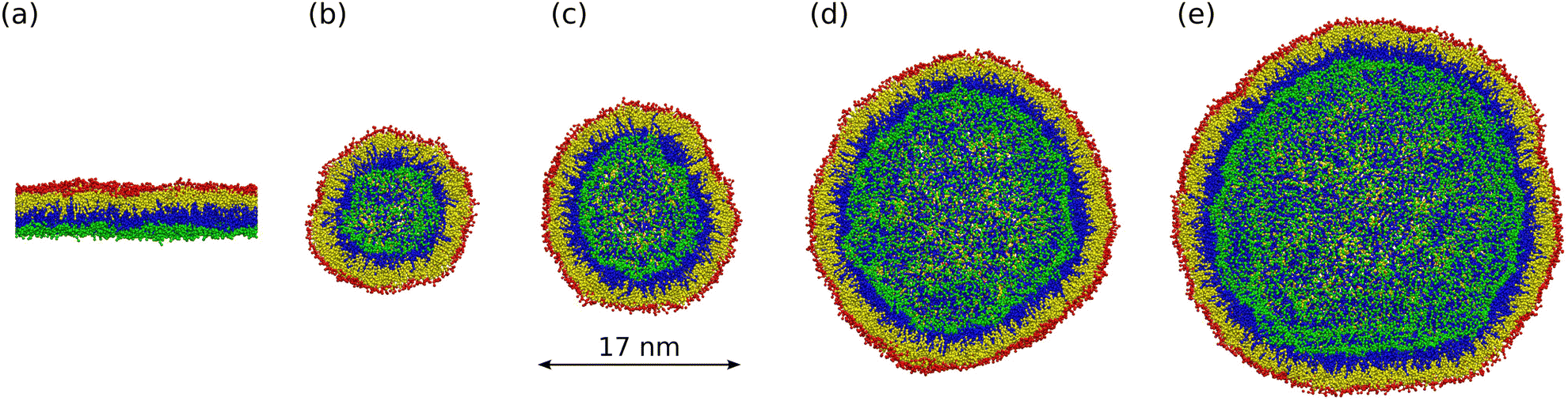

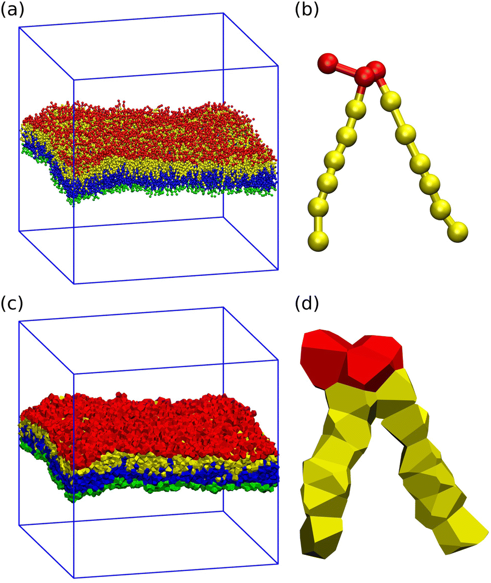
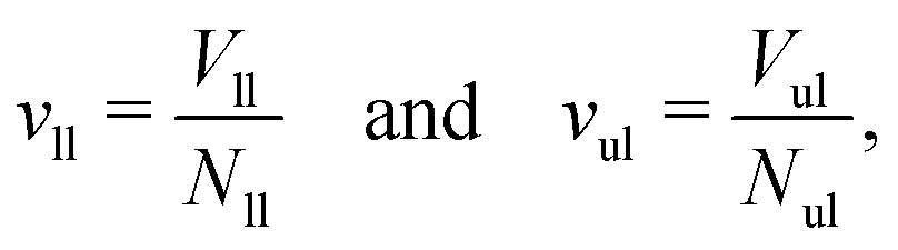
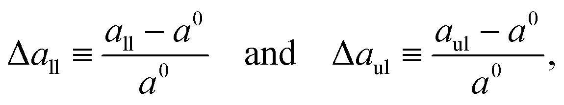

 ,
,  ,
,  , and
, and  ; and (c) Leaflet tensions versus projected area per lipid, ale. The filled data symbols represent those data that belong to the linear regime and fulfill the linearity condition |Δale| < KOLT/10K′. The gray shaded band indicates the 95% prediction band for the linear fit. The numerical values of the data are displayed in Table S3 (ESI†).