DOI:
10.1039/D3SM00334E
(Paper)
Soft Matter, 2023,
19, 5857-5868
Insights and guidelines to interpret forces and deformations at the nanoscale by using a tapping mode AFM simulator: dForce 2.0
Received
15th March 2023
, Accepted 19th May 2023
First published on 12th June 2023
Abstract
Amplitude modulation (tapping mode) AFM is the most versatile AFM mode for imaging surfaces at the nanoscale in air and liquid environments. However, it remains challenging to estimate the forces and deformations exerted by the tip. We introduce a new simulator environment to predict the values of the observables in tapping mode AFM experiments. The relevant feature of dForce 2.0 is the incorporation of contact mechanics models aimed to describe the properties of ultrathin samples. These models were essential to determine the forces applied on samples such as proteins, self-assembled monolayers, lipid bilayers, and few-layered materials. The simulator incorporates two types of long-range magnetic forces. The simulator is written in an open-source code (Python) and it can be run from a personal computer.
1. Introduction
Amplitude modulation AFM (AM–AFM), usually referred to as tapping mode AFM, is the most popular nanoscale microscopy method for imaging materials’ surfaces at high-spatial resolution in air and liquid environments.1–10 Among other features, AM–AFM supports the operation of high-speed11–15 and bimodal16–21 AFM modes, enables AFM phase imaging,22–27 facilitates the identification of energy dissipation processes28 and provides quantitative values of the energy dissipated on the sample at the nanoscale.29–32
The theory of tapping mode AFM is rather complex.1 It is usually presented in two versions. One version is devoted to describing experiments performed in air.1,2,33,34 The other version is aimed to describe experiments performed in liquid environments or, equivalently, with low quality factor microcantilever (Q ≤ 5).1,35–38
The nonlinear dependence of the force with the tip-surface distance gave rise to a rich variety of nonlinear dynamic properties,39–48 specifically, the coexistence of two or more steady-state solutions for the same set-point amplitude (bistability). This feature was commonly observed in tapping mode AFM operation.40,42 Sometimes, it was explained in terms of a competition between attractive and repulsive interaction regimes.2,48 The presence of higher harmonics in the tip's oscillation is another manifestation of nonlinearity.42,44–47
The main observables in AM–AFM, the amplitude and the phase shift, are averaged over an oscillation cycle. This feature added another layer of complexity because it prevented the direct (instantaneous) determination of the tip-sample force. To address this issue amplitude and phase shift-distance curves were obtained. These curves were converted into force–distance curves by solving an integral equation.49–51 Recently, several theoretical and experimental contributions have illustrated the evolution trends followed in AM–AFM.52–64
The dynamics of the tip motion in AM–AFM was far from intuitive. High spatial resolution images were obtained by either following a time-consuming trial and an error approach or by following a set of strict protocols. It was argued that the use of simulator environments might speed up AM–AFM data interpretation.65–67 In particular, dForce67 was developed as an open-source code to simulate the behaviour of tapping mode and bimodal observables.
The evolution experienced by the applications of amplitude modulation AFM in materials science, nanotechnology and molecular biology since 2015 has motivated a complete revision and upgrade of the capabilities of tapping mode AFM simulators. For example, nanomechanical mapping has become very common in materials science.26,68–73 In some cases, these measurements involved the characterization of ultrathin layers (≤10 nm) deposited on a rigid substrate. High-speed AFM provides a high-spatial resolution and real-time images of self-assembly processes.13,71–73 An understanding of the forces and the deformations in high-speed AFM requires the application of bottom-effect corrections.74 In addition, the discovery of room-temperature magnetic skyrmions75 has renewed the interest in applying magnetic force microscopy to characterize magnetic materials at the nanoscale.76–81
In this paper, we introduce the capabilities of dForce 2.0 to predict and simulate the force, the deformation and the spatial resolution at the nanoscale on a variety of nanoscale materials including ultrathin soft materials and magnetic samples. The code is suitable to simulate experiments performed in liquid or air environments. The code incorporates twenty-six force models (Fig. 1a). In particular, it includes some models aimed to describe the mechanical properties of ultrathin layers. The validity of these models was previously demonstrated theoretically and via numerical and finite element simulations.82–86 In short, the dForce 2.0 platform is designed to simulate the time and spatial dependencies of the observables and quantities measured using tapping and bimodal AFM methods. The simulations might be interpreted as predictions of experimental outcomes. In this way, dForce 2.0 will facilitate the selection of the optimum imaging parameters to maximize the spatial resolution while minimizing tip-sample deformations, distortions or damage.
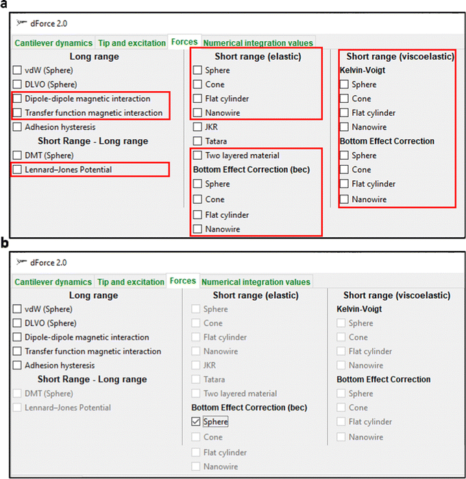 |
| | Fig. 1 (a) Graphical user interfaces of the force selection menu. The menu shows the interaction forces available in dForce 2.0. Enclosed in red boxes are the new interaction forces incorporated into the simulator. (b). Force menu that shows that the selection of the bottom-effect correction model for a sphere was compatible with three other interactions, such as van der Waals interactions, dipole–dipole interactions and transfer function magnetic forces. This feature was included to prevent unphysical combination force models. | |
2. General features and graphical user interfaces
Fig. 1a shows the capabilities of dForce 2.0 to simulate twenty-six interaction force models. In contact mechanics, the code includes Sneddon's models for a flat cylinder and a conical probe;87 Hertz's model88 and the nanowire model.83 More importantly, the code includes extensions of the above models to describe the forces and the deformations on experiments performed on ultrathin layers. In the AFM context, these extensions were called bottom effect corrections.26 The capabilities to simulate viscoelastic materials were significantly expanded by including the 3D Kelvin–Voigt model and its extension to describe the properties of soft matter layers and, in general, finite-thickness materials attached or deposited on a rigid substrate. The new version also includes two long-range magnetic forces and the Lennar-Jones force. To facilitate the speed of the simulations in laptops and personal computers, dForce 2.0 considers interaction force models which are expressed by analytical equations.
The dForce 2.0 platform offers the possibility of combining several interaction force models. To avoid meaningless calculations, dForce 2.0 restricts the combination of these models that were mutually compatible. This is achieved, once a force model is selected, by keeping active the models compatible with the first selection.
Fig. 1b illustrates the models compatible with the selection of short-range bottom-effect correction forces for a paraboloid. These models are van der Waals, DVLO, and magnetic force models and adhesion hysteresis. The compatibility issues were usually associated with the boundary conditions used to deduce the expressions.
In AM–AFM, the tip's oscillation contains two terms. One that decays with time (transient) and the other is a sinusoidal oscillation.1 In AM–AFM, the observables are determined from the sinusoidal solution. This assumption implies that the transient term had vanished. The code offers the possibility to estimate that time automatically by clicking the ‘optimum parameter’ option in the ‘numerical integration values’ menu.
The dForce 2.0 code can be downloaded from the link given in ref. 89. Running the program will create a folder, dForceproject-date-time. This folder will initially contain four files, such as a text file with the inputs of the simulation, and three excel files with spatial (zcdom1), time (tdom1) and frequency (wdom1) domain values. These files will be used to generate the graphical representations. These plots will be saved in the same folder. All the simulations performed in the same session will be saved in the same folder. The files, text, excel and graphs will be named sequentially (1, 2, etc.).
3. Bottom-effect corrections
To determine the forces applied on a thin sample either deposited (frictionless) or bonded to a rigid substrate required to apply the so-called bottom effect corrections.26,82–86 These corrections are essential to measure with accuracy the nanomechanical properties of different samples such as proteins,73 polymer-based thin films,25 lipid bilayers,74,90 and self-assembled monolayers.91 In fact, these corrections should also be applied to any method intended to measure the mechanical properties of a thin layer using a finite-size probe. However, most nanomechanical measurements were performed without including these corrections. The insights offered by dForce 2.0 simulations on ultrathin samples might contribute to understand the quantitative relevance of bottom-effect corrections. In the process, the code might facilitate the incorporation bottom-effect features into the nanomechanics toolbox.
In dForce 2.0, the bottom-effect corrections are implemented for the axisymmetric probe–sample interfaces schematized in Fig. 2. The code considers semi-infinite (Fig. 2a) and finite-thickness samples (Fig. 2b). Irrespective of the elastic or viscoelastic nature of the finite-thickness sample, the force might be decomposed into two terms:83,84
The first term
Fsemi expresses the reaction of the material as if it was semi-infinite. The second term
Fbec accounts for the thickness of the sample,
a is the contact radius and
h is the sample thickness. For the same indentation, the force exerted by a probe on a thin sample deposited on a rigid substrate increased by increasing the
a/
h ratio.
26,82–84 This equation leads to a counter-intuitive result. For the same sample thickness, the force increases by increasing the radius of the projected contact area. In other words, the force increases using larger probes.
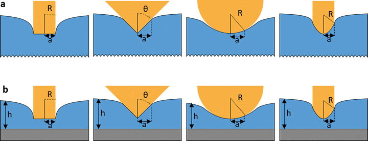 |
| | Fig. 2 Scheme of several probe–material interfaces simulated by dForce 2.0. (a) Interfaces for a semi-infinite material. Left-to-right, flat cylinder (radius R), cone (half-angle θ), sphere (radius R) and nanowire (radius R); h is the thickness of the layer and a is the radius of the projected contact area. (b) Interfaces for finite-thickness samples. The layers might be either bonded or deposited (frictionless) to the rigid substrate. Left-to-right, flat cylinder, cone, sphere and nanowire probes. | |
For an elastic material, Fsemi is determined by using the expressions deduced by Sneddon87 for a cone and a flat cylinder. For a probe ended in a hemisphere, the force is determined by using Hertz's model.88 For a nanowire, we use the expression deduced in ref. 83. For a viscoelastic material, Fsemi is determined by using the 3D Kelvin-Voigt expressions.84
3.1 Elastic materials
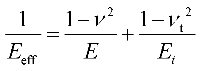
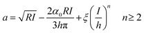
The force exerted on the elastic material was determined analytically for four axisymmetric probe geometries, such as the flat cylinder, cone, sphere and nanowire.83 In these expressions, the effective Young's modulus of the interface is given by| | 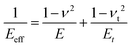 | (2) |
where E and Et, are, respectively, the Young's modulus of the sample and the tip; ν and νt are, respectively, the Poisson's ratio of the sample and the tip.
For a flat cylinder,83
| | 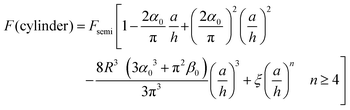 | (3) |
where
a is the radius
R of the cylinder and
h is the sample thickness. The expression ξ (
a/
h)
n is a polynomial which includes the correction terms with an exponent
n ≥ 4. The contribution of these terms to the total force can be neglected.
The force is applied by the flat cylinder on the semi-infinite (half-space) sample of Young's modulus E is given by
| | 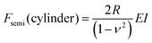 | (4) |
where
I is the sample deformation.
For a conical probe of half angle θ,83
| | 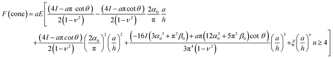 | (5) |
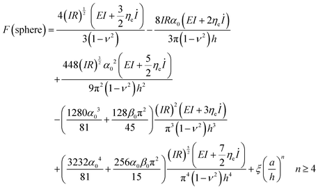
For a sphere (
I < R)
| | 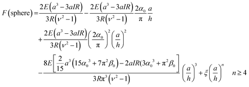 | (6) |
The force exerted using a nanoneedle tip as a function of the indentation is determined by
83| | 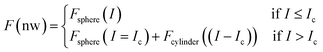 | (7) |
where
Ic defines the value where the contact radius coincided with the radius
R of the spherical cap of the nanowire.
The contact area between a probe and a finite-thickness sample depends also on the sample thickness for conical, parabolic and nanowire probes.83
For a cone, the contact radius
| | 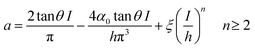 | (8) |
For a spherical probe (referred as sphere,
I < R),
| |  | (9) |
The coefficients
α0 and
β0 depend on the boundary conditions. The deduction is given in ref.
82. For a layer bonded to a rigid substrate,
| | 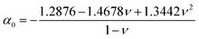 | (10) |
| | 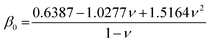 | (11) |
For a frictionless contact between the layer and the rigid substrate,
| | 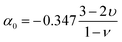 | (12) |
| |  | (13) |
The validity of the above expressions was verified by numerical and finite element simulations.
83–85
3.2 Two-layered uncompressible elastic materials
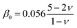
Ros and co-workers addressed the problem of determining the force exerted using a spherical probe on a system formed by the finite-thickness layer deposited on top of a deformable semi-infinite layer.85 For this system, the force is calculated by| | 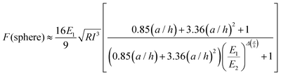 | (14) |
where the exponent Δ is given by| | 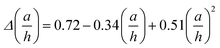 | (15) |
In eqn (14)E1 and E2 stand, respectively, for the Young's modulus of the top and bottom layers. The above equation provides a good description of the force exerted on a two-layered system as long as E1/E2 < 100 and ν1 = ν2 = 0.5.
3.3 Viscoelastic materials
In dForce 2.0, we have implemented the expressions deduced within the framework of the 3D Kelvin–Voigt model.84| | | Fsemi(I(t),t) = αI(t)β−1[EI(t) + βηeİ(t)] | (16) |
where α is the coefficient that depends on the probe geometry and sample properties; β is the coefficient that depends on the probe geometry; ηe is the elongation or compression viscosity coefficient. For many materials, there is a simple relationship between the elongation velocity and the shear viscosity η, ηe = 3η.92| | | F(I(t),t) = Fsemi + Fbec(a/h) | (17) |
For the cylinder of radius R, the force was given by| | 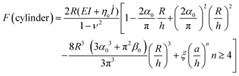 | (18) |
where a = R.
For a conical probe of half angle θ,
| | 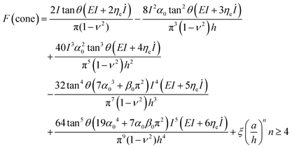 | (19) |
For a sphere (
I < R)
| |  | (20) |
The expression
ξ(
a/h)
n is a polynomial which includes the terms with an exponent
n ≥ 4. The contribution of these terms to the total force might be negligible.
3.4 Lateral resolution
A phenomenological definition of lateral resolution Lr is proposed by identifying the diameter of the region deformed by the tip as the lateral resolution.1,3,93 The above definition is valid for any AFM mode that involves the mechanical contact between the tip and the sample. Then,The force models discussed in the previous sections provide values of a as a function of the material properties, the indentation, and the tip radius (half angle for a conical tip).
3.5 Long-range magnetic interactions
Hartman deduced an expression to determine the force acting between two magnetic dipoles.93 In this model, the dipoles were oriented perpendicular to the sample surface (Fig. 1b) and then the force acting on the magnetized tip was approximated by94| | 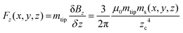 | (22) |
where Bz, mtip, and ms are, respectively, the component of the magnetic field in the direction perpendicular to the sample, the magnetic moment of the tip and the sample, μ0 is the permittivity of the vacuum, and zc is the average tip–sample distance.
Hug and colleagues have developed the tip–sample transfer function model to characterize the magnetic properties at the nanoscale.95,96 This model is widely used in magnetic and bimodal force microscopy applications. In this model, the force is expressed by
| | 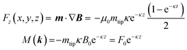 | (23) |
where
M(
k) is the Fourier transform of the sample magnetization
Mz(
r). The vectors
k and
r satisfy
| |  | (24) |
4. Results and discussion
4.1 Material system made of an elastic layer bonded to a rigid sample
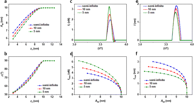
Fig. 3 shows the amplitude and the phase shift-distance curves obtained on the soft elastic material (E = 100 MPa) using a spherical probe (R = 5 nm). Specifically, the data compared the amplitude, the phase shift, the indentation and the maximum force obtained for the finite-thickness samples (5 and 10 nm) with those obtained on the semi-infinite sample. The amplitude and the phase shift decreases with zc. The simulations were performed in the repulsive regime. The variations are larger on the thinnest sample (5 nm) (Fig. 3a and b). This effect is related to the values of the instantaneous force exerted on the sample. For the same zc, the force is always higher in the thinnest sample (Fig. 3c). Similarly, the maximum force is always higher on the thinnest sample with the independence of the set-point amplitude (Fig. 3d). Paradoxically, the larger values of the indentation (instantaneous and maximum) are obtained on the semi-infinite sample (Fig. 3e and f). These findings contradict the predictions derived by Sneddon and Hertz's models where for the material characterized by E and ν, the force should increase with the indentation. Ultimately, the behavior measured on finite-thickness samples reflects the bottom-effect induced by the rigid substrate. The stress applied on the top surface of the layer propagates through the layer until it reached the rigid substrate. Then, it is reflected back to reach the probe. This effect increased the force. In eqn (3), (5) and (6), it is shown that for the same indentation and contact radius, the force would increase by decreasing h.
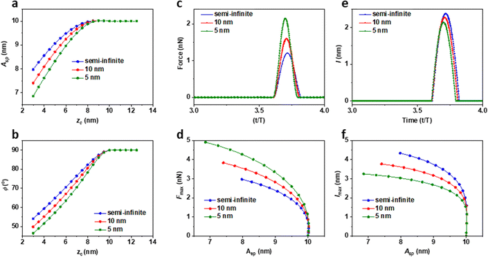 |
| | Fig. 3 Effect of the sample thickness on AM–AFM observables for an elastic material (E = 100 MPa; ν = 0.3). (a) Amplitude dependence of the average tip-surface distance. (b) Phase shift dependence of the average tip-surface distance. (c) Force as a function of time during an oscillation cycle (zc = 7.5 nm). (d) Maximum force for different Asp values. (e) Indentation as a function of time during an oscillation cycle (zc = 7.5 nm). (f) Indentation as a function of Asp. Parameters: R = 5 nm, f0 = 350 kHz, k = 0.3 N m−1, Q = 2, and Ao = 10 nm. | |
Fig. 4 shows the graphical user interfaces (GUIs) with the corresponding selections needed to perform the simulations discussed above. In step 4, by clicking the tab called optimized values, the program selected the number of periods needed to get rid of the transient term. Fig. 5 illustrates the procedure to obtain the graphs shown in Fig. 3.
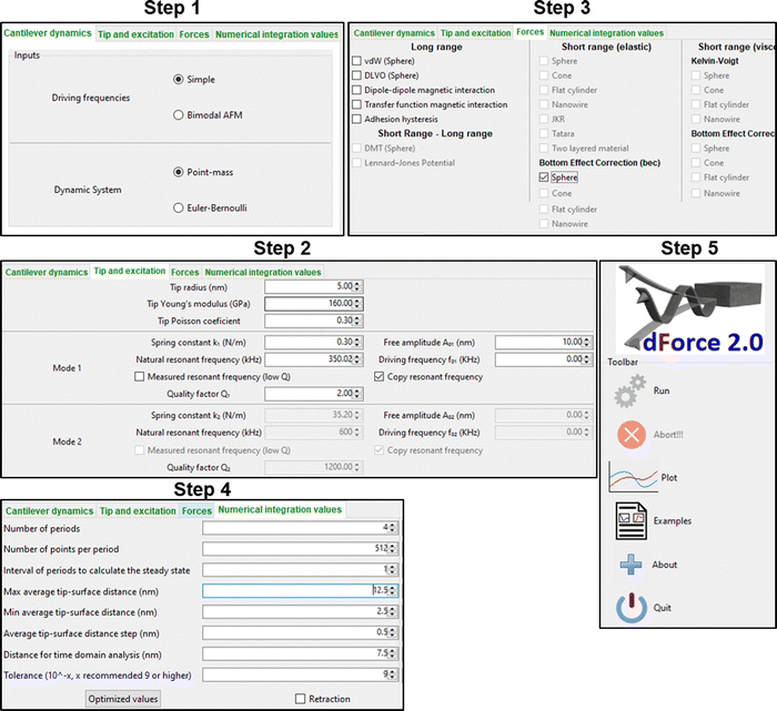 |
| | Fig. 4 Steps followed to generate the data shown in Fig. 3. | |
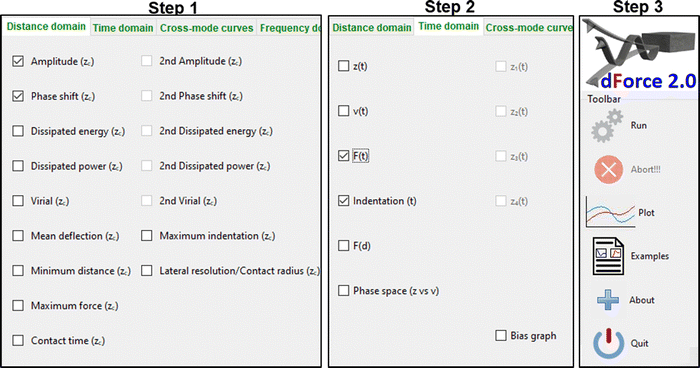 |
| | Fig. 5 Steps followed to generate the plots shown in Fig. 3. These steps were performed once the simulations described in Fig. 4 were accomplished. | |
4.2 Material system made of a viscoelastic layer attached to a rigid sample
Fig. 6 shows the amplitude and the phase shift-distance curves obtained on the soft viscoelastic material (E = 100 MPa and η = 2 Pa s) with a paraboloid (R = 5 nm). The amplitude, the phase shift, the indentation and the forces obtained on a 5 nm and 10 nm thick layers were compared with those obtained on the semi-infinite sample. For smaller zc values, the phase shifts calculated on the thinnest samples are very close or even larger than the one calculated on the semi-infinite sample. This result is a direct consequence of the viscous response (see below). In general, the comparison followed the trends observed by their elastic counterparts. The largest force is measured on the thinnest sample (Fig. 6c and d) while the opposite occurs for the indentation (Fig. 6e and f). The largest variations are observed in the thinner sample. The presence of the viscous force enhances the decrease of the amplitude and the phase shift with respect to the elastic case (Fig. 3). In addition, the viscosity attenuates the differences observed in the phase shift values due to the sample thickness.
 |
| | Fig. 6 Effect of the sample thickness on AM–AFM observables for a viscoelastic material (E = 100 MPa; η = 2 Pa s; and ν = 0.3). (a) Amplitude dependence of the average tip-surface distance. (b) Phase shift dependence of the average tip-surface distance. (c) Force as a function of time during an oscillation cycle (zc = 7.5 nm). (d) Maximum force for different Asp values. (e) Indentation as a function of time during an oscillation cycle (zc = 7.5 nm). (f) Indentation as a function of Asp. Parameters: R = 5 nm, f0 = 350 kHz, k = 0.3, Q = 2, and Ao = 10 nm. | |
Viscoelastic systems dissipate energy. This is illustrated in Fig. 7 by showing the hysteresis loop in the force–distance curves. The dissipated energy per cycle is the area enclosed by the force–distance curve. Higher forces and higher energy dissipation values were measured on the thinnest layer. The energy dissipated in the sample by the viscous force introduced an additional phase shift (Fig. 6b). The phase shift associated with energy dissipation was larger on the 5 nm sample because the energy dissipation was also larger (Fig. 7).25,28–30
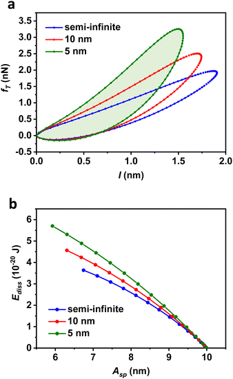 |
| | Fig. 7 (a) Force-indentation curves obtained on a viscoelastic material at zc = 7.5 nm. The amount of energy dissipated per cycle in the viscoelastic sample (h = 5 nm) was the area shaded in light green. (b) Energy dissipation as a function of Asp for the above system. Parameters: E = 100 MPa, ηG = 2 Pa s, ν = 0.3, R = 5 nm, f0 = 350 kHz, k = 0.3, Q = 2, and Ao = 10 nm. | |
4.3 Magnetic interactions
Fig. 8a shows the scheme of a magnetic force microscopy measurement performed in the lift mode. The dForce 2.0 platform offers two models to determine magnetic forces. The dipole–dipole model is more appropriate to describe magnetic systems characterized by domains with a uniformed magnetization while the transfer function model function is proposed to describe magnetic systems where the magnetization shows some variations across the magnetic domain.
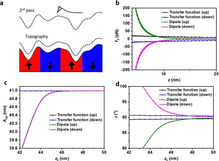 |
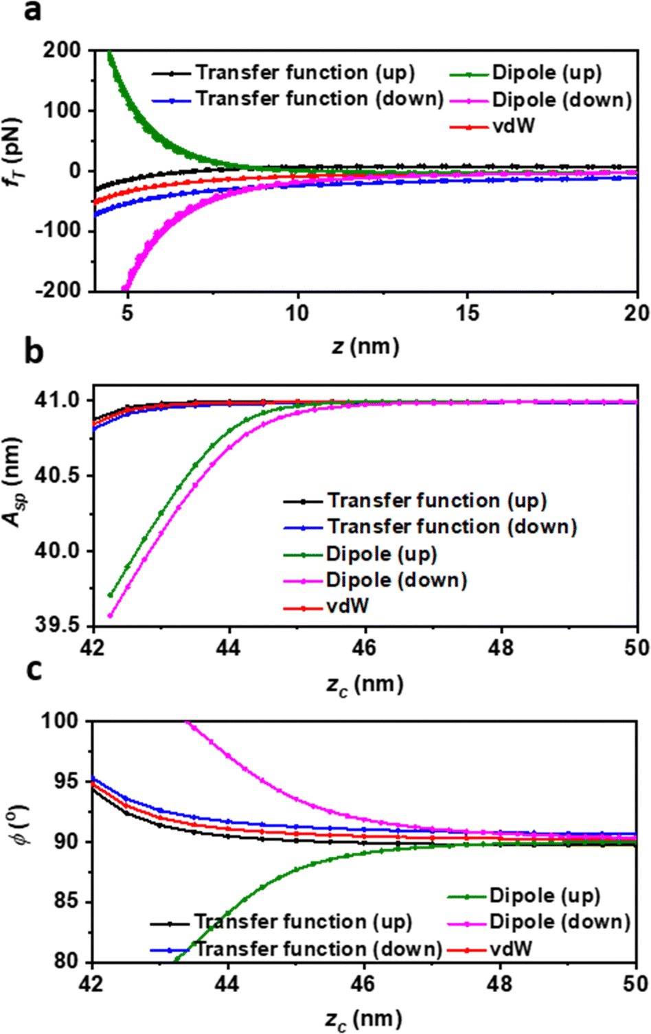
| | Fig. 8 (a) Scheme of a magnetic force microscopy measurement. (b) Force–distance curves for different magnetic forces. The forces (up and down) are symmetric with respect to the horizontal axis. (c) Amplitude-distance curves for the forces shown in (a). Note that for weak magnetic forces, the changes in the amplitude at relatively large tip-sample distances (≥40 nm) are almost negligible. (d) Phase shift-distance curves for the forces shown in (a). Parameters: R = 50 nm, f0 = 79 kHz, k = 3.4 N m−1, Q = 160, and Ao = 41 nm. Transfer function model B (sample) = ±10 mT; mtip = 5 emu, ms = 0.0003 emu. | |
Fig. 8b shows the dependence of the force with respect to the tip-sample separation for dipole–dipole and delocalized magnetic interactions. The sign of the force depends on the alignment of the tip's and sample magnetic fields, parallel or anti-parallel. The forces are symmetric with respect to the horizontal axis (zero force). In the case of the transfer function model, the magnetic field on the sample was 10 mT (up) and – 10 mT (down). For the dipole–dipole interaction mode, ms = 0.0003 emu and mtip = 5 emu.
Irrespective of the attractive or the repulsive character of the magnetic interactions, an increase (absolute value) of the force causes a decrease of the amplitude (Fig. 8c). We note that for weak magnetic forces, here simulated by the transfer function model, the changes in the amplitude at relatively large tip-sample distances (≥40 nm) are almost negligible. On the other hand, the phase shift is very sensitive to both the strength of the force and its sign. Attractive forces decrease the phase shift while repulsive forces produce an increase. The numerical results were consistent with the theory linking the phase shifts to the force gradients.97 This feature is commonly exploited in MFM to determine the alignment of the sample's magnetic domains.
Long-range van der Waals interactions might be unavoidable in a magnetic force microscopy measurement. For this reason, we include simulations with van der Waals forces (R = 50 nm and H = 0.6 eV). The presence of van der Waals forces breaks the symmetry of the magnetic interaction (Fig. 9a). This is clearly seen in the simulations performed using the transfer function model. Fig. 9b and (c) show, respectively, the amplitude and phase shift-distance curves for the forces depicted in (a). Whenever magnetic and van der Waals forces are comparable, the phase shift associated with the magnetic interaction (the transfer function model) might be hard to distinguish the phase shift associated with van der Waals interactions (Fig. 9c).
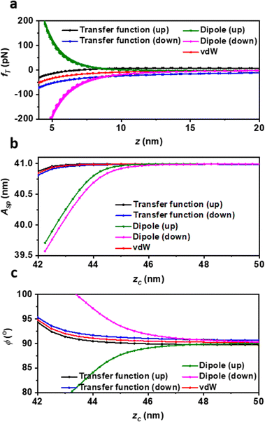 |
| | Fig. 9 (a) Force–distance curves for dipole–dipole and transfer function model magnetic forces in the presence of a van der Waals force. The van der Waals force breaks the symmetry of the magnetic interaction (up versus down). (b) Amplitude-distance curves for the forces shown in (a). (c) Phase shift-distance curves for the forces shown in (a). Parameters: R = 50 nm, f0 = 79 kHz, k = 3.4 N m−1, Q = 160, and Ao = 41 nm. Transfer function model B (sample) = ±10 mT; mtip = 5 emu, ms = 0.0003 emu; H = 0.63 eV. | |
4.4 Forces, deformations and spatial resolution
It is well known that the force applied by the tip on a soft material might introduce sample distortions or damage.1,43,98 Commonly, an AFM user relies on empirical observations to establish the optimum imaging parameters (free and set-point values) to perform an experiment. To illustrate the benefits of using dForce 2.0 to facilitate the selection of the imaging parameters, we have simulated the outputs of the tapping mode AFM measurement as a function of imaging parameters.
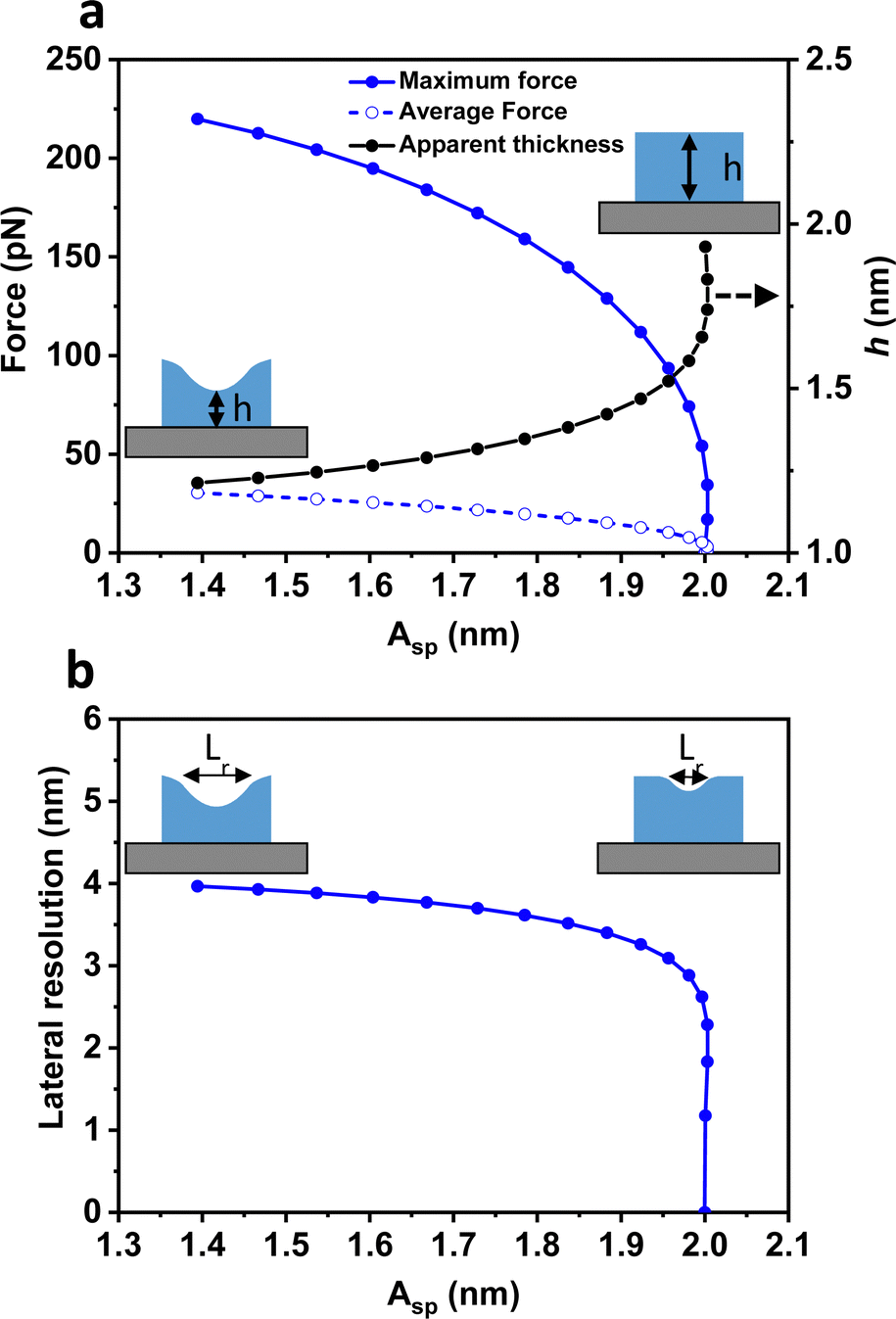
Fig. 10a shows the values of the maximum force, the average force and the deformation as a function of the set-point amplitude. The force increases from 0 to 225 pN by reducing the value of Asp from A0 (2 nm) to 1.4 nm. At the same time, the deformation increases from 0 nm to 0.8 nm. The latter value implies a significant compression (40%) of the sample. It has been experimentally shown that deformations amounting more than 30% of the nominal diameter of a protein were associated with the existence of irreversible plastic deformations.99 Therefore, the above simulation indicates that the use of an Asp value below 1.5 nm (Asp/Ao ≤ 0.85) might be associated with an irreversible sample deformation.
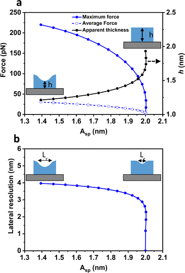 |
| | Fig. 10 (a) Maximum force, average force and apparent thickness as a function of the set-point amplitude. (b) Spatial resolution. Parameters of the simulation for the tip and the sample: R = 5 nm, f0 = 29 kHz, k = 0.084 N m−1, Q = 2.0, Ao = 2 nm, E = 50 MPa, and h = 2 nm. | |
The lack of an analytical expression to calculate the force has led to use the average force to estimate the force applied on the sample. Fig. 10a shows that this approximation should not be used. The average force over an oscillation significantly underestimates the maximum force. For example, for an Asp = 1.6, the average force was 8-fold smaller than the maximum force.
Fig. 10b shows that the lateral resolution of the experiment will change from ≈3 nm to ≈1 nm by decreasing the Asp value from 1.9 to 1.4 nm. The material was characterized by a thickness of 2 nm and a Young's modulus of 50 MPa. The simulation did not include van der Waals forces. The tip was a sphere of R = 5 nm.
5. Conclusions
We have developed new capabilities for simulating tapping mode and bimodal AFM experiments. The dForce 2.0 platform is suitable to predict the observables of amplitude modulation AFM under a variety of short and long-range forces. The simulator includes a number of contact mechanics models suitable to provide insights into forces and deformations in elastic and viscoelastic materials. A key feature is the incorporation of bottom-effect corrections to describe the experiments performed on the finite thickness samples attached or deposited on a rigid substrate. These corrections are essential to describe with numerical accuracy the forces and the deformations exerted by the AFM tip on biomolecules and thin soft matter layers. In particular, dForce 2.0 is suitable to describe experiments are performed by using bimodal and high-speed AFM modes.
The simulator incorporates two models to determine long-range magnetic interactions. The results show the interplay between van der Waals and magnetic forces to influence the phase shift, which is the main observable in the magnetic force microscopy experiment.
The simulator is designed to be run in personal computers or laptops. It is written in an open-source code (python) and can be freely downloaded from the link in ref. 89. The predictive features of dForce 2.0 might be exploited to plan and to interpret nanoscale measurements for a variety of interactions and environments.
Conflicts of interest
There are no conflicts to declare.
Acknowledgements
Financial supports from the Ministerio de Ciencia e Innovación (PID2019-106801GB-I00/AEI/10.13039/501100011033) and CSIC 202050E013 are acknowledged.
References
-
R. Garcia, Amplitude Modulation Atomic Force Microscopy, Wiley-VCH Verlag GmbH & Co. KGaA, Weinheim, Germany, 2010 Search PubMed.
- R. Garcia and A. San Paulo, Phys. Rev. B: Condens. Matter Mater. Phys., 1999, 60, 4961–4967 CrossRef CAS.
- Y. Gan, Surf. Sci. Rep., 2009, 64, 99–121 CrossRef CAS.
- M. R. Uhlig, D. Martin-Jimenez and R. Garcia, Nat. Commun., 2019, 10, 2606 CrossRef PubMed.
- S. Su, I. Siretanu, D. Ende, B. Mei, G. Mul and F. Mugele, Adv. Mater., 2021, 33, 2106229 CrossRef CAS PubMed.
- C. Möller, M. Allen, V. Elings, A. Engel and D. J. Müller, Biophys. J., 1999, 77, 1150–1158 CrossRef.
- P. Ares, M. E. Fuentes-Perez, E. Herrero-Galán, J. M. Valpuesta, A. Gil, J. Gomez-Herrero and F. Moreno-Herrero, Nanoscale, 2016, 8, 11818–11826 RSC.
- H. Pyles, S. Zhang, J. J. De Yoreo and D. Baker, Nature, 2019, 571, 251–256 CrossRef CAS.
- V. V. Korolkov, A. Summerfield, A. Murphy, D. B. Amabilino, K. Watanabe, T. Taniguchi and P. H. Beton, Nat. Commun., 2019, 10, 1537 CrossRef PubMed.
- D. Klinov and S. Magonov, Appl. Phys. Lett., 2004, 84, 2697–2699 CrossRef CAS.
- N. Kodera, D. Yamamoto, R. Ishikawa and T. Ando, Nature, 2010, 468, 72–76 CrossRef CAS.
- T. Ando, Nanotechnology, 2012, 23, 062001 CrossRef PubMed.
- T. Ando, T. Uchihashi and S. Scheuring, Chem. Rev., 2014, 114, 3120–3188 CrossRef CAS PubMed.
- Y.-C. Lin, Y. R. Guo, A. Miyagi, J. Levring, R. MacKinnon and S. Scheuring, Nature, 2019, 573, 230–234 CrossRef CAS PubMed.
- A. Valbuena, S. Maity, M. G. Mateu and W. H. Roos, ACS Nano, 2020, 14, 8724–8734 CrossRef CAS PubMed.
- T. R. Rodriguez and R. Garcia, Appl. Phys. Lett., 2004, 84, 449–451 CrossRef CAS.
- R. Garcia and R. Proksch, Eur. Polym. J., 2013, 49, 1897–1906 CrossRef CAS.
- D. Ebeling and S. D. Solares, Nanotechnology, 2013, 24, 135702 CrossRef PubMed.
- S. Santos, C.-Y. Lai, T. Olukan and M. Chiesa, Nanoscale, 2017, 9, 5038–5043 RSC.
- S. Benaglia, V. G. Gisbert, A. P. Perrino, C. A. Amo and R. Garcia, Nat. Protoc., 2018, 13, 2890–2907 CrossRef CAS PubMed.
- M. Kocun, A. Labuda, W. Meinhold, I. Revenko and R. Proksch, ACS Nano, 2017, 11, 10097–10105 CrossRef CAS PubMed.
- R. Garcia, J. Tamayo, M. Calleja and F. Garcia, Appl. Phys. A: Mater. Sci. Process., 1998, 66, S309–S312 CrossRef CAS.
- A. Knoll, R. Magerle and G. Krausch, J. Chem. Phys., 2004, 120, 1105–1116 CrossRef CAS PubMed.
- K. Voïtchovsky, J. J. Kuna, S. A. Contera, E. Tosatti and F. Stellacci, Nat. Nanotechnol., 2010, 5, 401–405 CrossRef PubMed.
- J. Raybin, J. Ren, X. Chen, R. Gronheid, P. F. Nealey and S. J. Sibener, Nano Lett., 2017, 17, 7717–7723 CrossRef CAS PubMed.
- R. Garcia, Chem. Soc. Rev., 2020, 49, 5850–5884 RSC.
- F. Lavini, F. Cellini, M. Rejhon, J. Kunc, C. Berger, W. de Heer and E. Riedo, J. Phys. Chem. Mater., 2020, 3, 024005 CAS.
- R. Garcia, C. J. Gómez, N. F. Martinez, S. Patil, C. Dietz and R. Magerle, Phys. Rev. Lett., 2006, 97, 016103 CrossRef CAS PubMed.
- J. Tamayo and R. Garcia, Appl. Phys. Lett., 1998, 73, 2926–2928 CrossRef CAS.
- B. Anczykowski, B. Gotsmann, H. Fuchs, J. P. Cleveland and V. B. Elings, Appl. Surf. Sci., 1999, 140, 376–382 CrossRef CAS.
- N. F. Martínez and R. García, Nanotechnology, 2006, 17, S167 CrossRef PubMed.
- S. Santos, V. Barcons, A. Verdaguer, J. Font, N. H. Thomson and M. Chiesa, Nanotechnology, 2011, 22, 345401 CrossRef PubMed.
- A. San Paulo and R. Garcia, Phys. Rev. B: Condens. Matter Mater. Phys., 2002, 66, 041406 CrossRef.
- H. Hölscher, D. Ebeling and U. D. Schwarz, J. Appl. Phys., 2006, 99, 084311 CrossRef.
- E. T. Herruzo and R. Garcia, Appl. Phys. Lett., 2007, 91, 143113 CrossRef.
- D. Kiracofe and A. Raman, J. Appl. Phys., 2010, 107, 033506 CrossRef.
- J. Tamayo, Appl. Phys. Lett., 1999, 75, 3569–3571 CrossRef CAS.
- X. Xu, J. Melcher, S. Basak, R. Reifenberger and A. Raman, Phys. Rev. Lett., 2009, 102, 060801 CrossRef PubMed.
- M. Marth, D. Maier, J. Honerkamp, R. Brandsch and G. Bar, J. Appl. Phys., 1999, 85, 7030–7036 CrossRef CAS.
- R. Garcia and A. San Paulo, Phys. Rev. B: Condens. Matter Mater. Phys., 2000, 61, R13381 CrossRef CAS.
- A. Raman, J. Melcher and R. Tung, Nano Today, 2008, 3, 20–27 CrossRef CAS.
- R. W. Stark, Mater. Today, 2010, 13, 24–32 CrossRef.
- A. San Paulo and R. Garcia, Biophys. J., 2000, 78, 1599–1605 CrossRef CAS.
- T. R. Rodriguez and R. Garcia, Appl. Phys. Lett., 2002, 80, 1646–1648 CrossRef CAS.
- O. Sahin, C. F. Quate, O. Solgaard and A. Atalar, Phys. Rev. B: Condens. Matter Mater. Phys., 2004, 69, 165416 CrossRef.
- J. Legleiter, M. Park, B. Cusick and T. Kowalewski, Proc. Natl. Acad. Sci. U. S. A., 2006, 103, 4813–4818 CrossRef CAS.
- K. Voïtchovsky, Phys. Rev. E, 2013, 88, 022407 CrossRef PubMed.
- B. Anczykowski, D. Krüger and H. Fuchs, Phys. Rev. B: Condens. Matter Mater. Phys., 1996, 53, 15485–15488 CrossRef CAS PubMed.
- H. Hölscher, Appl. Phys. Lett., 2006, 89, 123109 CrossRef.
- M. Lee and W. Jhe, Phys. Rev. Lett., 2006, 97, 036104 CrossRef.
- A. F. Payam, D. Martin-Jimenez and R. Garcia, Nanotechnology, 2015, 26, 185706 CrossRef.
- D. Martin-Jimenez and R. Garcia, J. Phys. Chem. Lett., 2017, 8, 5707–5711 CrossRef CAS PubMed.
- M. G. Ruppert, D. M. Harcombe, M. R. Ragazzon, S. O. Moheimani and A. J. Fleming, Beilstein J. Nanotechnol., 2017, 8, 1407–1426 CrossRef CAS PubMed.
- S. Kim, J.-H. Ko and W. Jhe, Phys. Rev. Lett., 2021, 126, 076804 CrossRef CAS.
- D. B. Haviland, Curr. Opin. Colloid Interface Sci., 2017, 27, 74–81 CrossRef CAS.
- A. Keyvani, H. Sadeghian, H. Goosen and F. van Keulen, Appl. Phys. Lett., 2018, 112, 163104 CrossRef.
- X. Hu, W. Nanney, K. Umeda, T. Ye and A. Martini, Langmuir, 2018, 34, 9627–9633 CrossRef CAS PubMed.
- P.-A. Thorén, R. Borgani, D. Forchheimer, I. Dobryden, P. M. Claesson, H. G. Kassa, P. Leclère, Y. Wang, H. M. Jaeger and D. B. Haviland, Phys. Rev. Appl., 2018, 10, 024017 CrossRef.
- T. Wagner, J. Appl. Phys., 2019, 125, 044301 CrossRef.
- N. H. Shaik, R. G. Reifenberger and A. Raman, Nanotechnology, 2020, 31, 455502 CrossRef CAS PubMed.
- S. Santos, K. Gadelrab, C.-Y. Lai, T. Olukan, J. Font, V. Barcons, A. Verdaguer and M. Chiesa, J. Appl. Phys., 2021, 129, 134302 CrossRef CAS.
- M. McCraw, B. Uluutku and S. Solares, Rep. Mec. Eng., 2021, 2, 156–179 CrossRef.
- A. Chandrashekar, P. Belardinelli, M. A. Bessa, U. Staufer and F. Alijani, Nanoscale Adv., 2022, 4, 2134–2143 RSC.
- A. F. Payam, A. Morelli and P. Lemoine, Appl. Surf. Sci., 2021, 536, 147698 CrossRef CAS.
- J. Melcher, S. Hu and A. Raman, Rev. Sci. Instrum., 2008, 79, 061301 CrossRef PubMed.
- D. Kiracofe, J. Melcher and A. Raman, Rev. Sci. Instrum., 2012, 83, 013702 CrossRef PubMed.
- H. V. Guzman, P. D. Garcia and R. Garcia, Beilstein J. Nanotechnol., 2015, 6, 369–379 CrossRef CAS PubMed.
- H. K. Nguyen, X. Liang, M. Ito and K. Nakajima, Macromolecules, 2018, 51, 6085–6091 CrossRef CAS.
- G. Stan and S. W. King, J. Vac Sci. Tech. B, 2020, 38, 060801 CrossRef CAS.
- D. W. Collinson, R. J. Sheridan, M. J. Palmeri and L. C. Brinson, Prog. Polym. Sci., 2021, 119, 101420 CrossRef CAS.
- J. Chen, E. Zhu, J. Liu, S. Zhang, Z. Lin, X. Duan, H. Heinz, Y. Huang and J. J. De Yoreo, Science, 2018, 362, 1135–1139 CrossRef CAS PubMed.
- J. Strasser, R. N. de Jong, F. J. Beurskens, J. Schuurman, P. W. Parren, P. Hinterdorfer and J. Preiner, ACS Nano, 2019, 14, 2739–2750 CrossRef PubMed.
- V. G. Gisbert, S. Benaglia, M. R. Uhlig, R. Proksch and R. Garcia, ACS Nano, 2021, 15, 1850–1857 CrossRef CAS PubMed.
- V. G. Gisbert and R. Garcia, ACS Nano, 2021, 15, 20574–20581 CrossRef CAS PubMed.
- S. Woo, K. Litzius, B. Krüger, M.-Y. Im, L. Caretta, K. Richter, M. Mann, A. Krone, R. M. Reeve, M. Weigand, P. Agrawal, I. Lemesh, M.-A. Mawass, P. Fischer, M. Kläui and G. S. Beach, Nat. Mater., 2016, 15, 501–506 CrossRef CAS PubMed.
- A. Hrabec, J. Sampaio, M. Belmeguenai, I. Gross, R. Weil, S. M. Chérif, A. Stashkevich, V. Jacques, A. Thiaville and S. Rohart, Nat. Commun., 2017, 8, 15765 CrossRef CAS PubMed.
- W. Legrand, D. Maccariello, N. Reyren, K. Garcia, C. Moutafis, C. Moreau-Luchaire, S. Collin, K. Bouzehouane, V. Cros and A. Fert, Nano Lett., 2017, 17, 2703–2712 CrossRef CAS PubMed.
- K.-Y. Meng, A. S. Ahmed, M. Baćani, A.-O. Mandru, X. Zhao, N. Bagués, B. D. Esser, J. Flores, D. W. McComb, H. J. Hug and F. Yang, Nano Lett., 2019, 19, 3169–3175 CrossRef CAS PubMed.
- Y. Feng, P. M. Vaghefi, S. Vranjkovic, M. Penedo, P. Kappenberger, J. Schwenk, X. Zhao, A. O. Mandru and H. J. Hug, J. Magn. Magn. Mater., 2022, 551, 169073 CrossRef CAS.
- V. G. Gisbert, C. A. Amo, M. Jaafar, A. Asenjo and R. Garcia, Nanoscale, 2021, 13, 2026–2033 RSC.
- N. H. Freitag, C. F. Reiche, V. Neu, P. Devi, U. Burkhardt, C. Felser, D. Wolf, A. Lubk, B. Büchner and T. Mühl, Commun. Phys., 2023, 6, 11 CrossRef CAS.
- E. K. Dimitriadis, F. Horkay, J. Maresca, B. Kachar and R. S. Chadwick, Biophys. J., 2002, 82, 2798–2810 CrossRef CAS PubMed.
- P. D. Garcia and R. Garcia, Biophys. J., 2018, 114, 2923–2932 CrossRef CAS PubMed.
- P. D. Garcia and R. Garcia, Nanoscale, 2018, 10, 19799–19809 RSC.
- B. L. Doss, K. Rahmani Eliato, K. Lin and R. Ros, Soft Matter, 2019, 15, 1776–1784 RSC.
- I. Argatov, X. Jin and G. Mishuris, J. R. Soc., Interface, 2023, 20, 20220857 CrossRef.
- I. N. Sneddon, Int. J. Eng. Sci., 1965, 3, 47–57 CrossRef.
-
K. L. Johnson, Contact mechanics, Cambridge University Press, 2003 Search PubMed.
- To download dForce 2.0 follow the instructions indicated in, https://wp.icmm.csic.es/forcetool/dforce-2-0/.
- E. N. Athanasopoulou, N. Nianias, Q. K. Ong and F. Stellacci, Nanoscale, 2018, 10, 23027–23036 RSC.
- S. Chiodini, S. Ruiz-Rincón, P. D. Garcia, S. Martin, K. Kettelhoit, I. Armenia, D. B. Werz and P. Cea, Small, 2020, 16, 2000269 CrossRef CAS PubMed.
-
N. W. Tschoegl, The Phenomenological Theory of Linear Viscoelastic Behavior: An Introduction, Springer Berlin Heidelberg, Berlin, Heidelberg, 1989 Search PubMed.
- T. P. Weihs, Z. Nawaz, S. P. Jarvis and J. B. Pethica, Appl. Phys. Lett., 1991, 50, 3536 CrossRef.
- U. Hartmann, Annu. Rev. Mater. Sci., 1999, 29, 53–87 CrossRef CAS.
- H. J. Hug, B. Stiefel, P. J. van Schendel, A. Moser, R. Hofer, S. Martin, H.-J. Güntherodt, S. Porthun, L. Abelmann, J. C. Lodder, G. Bochi and R. C. O’Handley, J. Appl. Phys., 1998, 83, 5609–5620 CrossRef CAS.
-
E. Meyer, H. J. Hug and R. Bennewitz, Scanning Probe Microscopy: Lab on a tip, Springer-Verlag, Berlin, 2004 Search PubMed.
- C. Dietz, E. T. Herruzo, J. R. Lozano and R. Garcia, Nanotechnology, 2011, 22, 125708 CrossRef PubMed.
- A. Knoll, R. Magerle and G. Krausch, Macromolecules, 2001, 34, 4159–4165 CrossRef CAS.
- A. P. Perrino and R. Garcia, Nanoscale, 2016, 8, 9151–9158 RSC.
|
| This journal is © The Royal Society of Chemistry 2023 |
Click here to see how this site uses Cookies. View our privacy policy here. 
 Open Access Article
 This Open Access Article is licensed under a Creative Commons Attribution-Non Commercial 3.0 Unported Licence
 and
Ricardo
Garcia
and
Ricardo
Garcia