
 Open Access Article
 This Open Access Article is licensed under a Creative Commons Attribution-Non Commercial 3.0 Unported Licence
Dynamic mechanical analysis of suspended soft bodies via hydraulic force spectroscopy†
Massimiliano
Berardi
 *ab,
Kajangi
Gnanachandran
c,
Jieke
Jiang
d,
Kevin
Bielawski
b,
Claas W.
Visser
d,
Małgorzata
Lekka
c and
B. Imran
Akca
a
*ab,
Kajangi
Gnanachandran
c,
Jieke
Jiang
d,
Kevin
Bielawski
b,
Claas W.
Visser
d,
Małgorzata
Lekka
c and
B. Imran
Akca
a
aLaserLab, Department of Physics and Astronomy, Vrije Universiteit Amsterdam, De Boelelaan 1081, 1081 HV, Amsterdam, The Netherlands. E-mail: massimiliano.berardi@optics11life.com
bOptics11, Hettenheuvelweg 37-39, 1101 BM, Amsterdam, The Netherlands
cDepartment of Biophysical Microstructures, Institute of Nuclear Physics, Polish Academy of Sciences, PL-31342, Kraków, Poland
dEngineering Fluid Dynamics group, Department of Thermal and Fluid Engineering, Faculty of Engineering Technology, University of Twente, 7500 AE, Enschede, The Netherlands
First published on 8th November 2022
Abstract
The rheological characterization of soft suspended bodies, such as cells, organoids, or synthetic microstructures, is particularly challenging, even with state-of-the-art methods (e.g. atomic force microscopy, AFM). Providing well-defined boundary conditions for modeling typically requires fixating the sample on a substrate, which is a delicate and time-consuming procedure. Moreover, it needs to be tuned for each chemistry and geometry. Here, we validate a novel technique, called hydraulic force spectroscopy (HFS), against AFM dynamic indentation taken as the gold standard. Combining experimental data with finite element modeling, we show that HFS gives results comparable to AFM microrheology over multiple decades, while obviating any sample preparation requirements.
1 Introduction
Micro-scale particles such as hydrogel microspheres and encapsulated droplets are widely used in the food industry, in medical applications and biology. The behavior and functionality of these particles is critically affected by their mechanical properties. For instance, hydrogels synthesized under different conditions can exhibit different mechanical properties as a consequence of structural differences.1–3 On top of this, the mechanical properties of biological structures such as cells can be used as label-free biomarkers to differentiate their physiological and pathological states.4Modeling and predicting the dynamic behavior of soft particles requires understanding of their rheological properties, i.e. their storage and loss moduli. This can also be used as a relatively simple proxy to evaluate other properties of interest, such as degradation dynamics,5 fracture toughness,6 and crystalline content.7 Atomic force microscopy (AFM), via dynamic nanoindentation, is the most common method used for probing these materials. However, characterization of spherical and suspended bodies such as microbeads, oocytes, spheroids, and organoids can be very challenging, partially due to their geometries. Such samples need to be stabilized e.g. by partially embedding them in a substrate, or coating the bottom of a dish with adhesives, or micromanufacturing trapping geometries. These procedures have to be tightly controlled so that compliance in the system (e.g. sample rotation, uncertainties in the contact area, trapping substrate has a stiffness comparable to that of the sample) are not erroneously interpreted as variations in characteristics of the sample. Owing to the chemical and physical variability of these samples, such preparation protocols need to be tuned each time. Additionally, in some cases the mechanical characterization may not be an end point measurement, making this route hardly practical. For example, in in vitro fertilization procedures, mechanical markers can be used to assess the quality of oocytes.8
Although there are a few techniques that allow measuring suspended samples (namely, micropipette aspiration (MPA),9 optical tweezers,10 and microfluidics-based approaches11,12), they are limited either in terms of spatial and temporal resolution, or in the range of applicable loads. Furthermore, previous studies13,14 found inconsistencies when testing the same samples via different methods, even when they could be reasonably assumed homogeneous and isotropic at multiple scales.15 This could be due to the shortcomings in the modeling and experimental protocols employed to extract their mechanical properties. Understanding the nature of these inconsistencies is important, especially when these methods are employed on biological samples. Previous research showed that the measured properties depend strongly on the scale/type of measurement.4,16 Usually, this is related to the different levels of influence of the probed constituents,4,13 or to poro- and viscoelasticity effects.17 However, appropriate quantification is still required.
Recently, we proposed a new approach to MPA that can help shed light on the origin of some of these measurement discrepancies.18 Specifically, previous works comparing MPA to other testing methods limited the analysis to quasi static properties.13,14 Thanks to the improvements in both temporal and spatial resolution, HFS can probe material behavior non-destructively at very low strain levels, and with enough temporal resolution to accurately capture the viscoelastic responses. Moreover, thanks to the possibility of performing closed-loop operations, HFS can perform dynamic mechanical analysis, which allows probing specific frequencies directly, without the need for a priori knowledge or assumptions about the frequency dependent material behavior.
In a traditional MPA experiment, the sample is captured at the distal end of a tapered glass capillary, by applying a negative pressure either through a pump or by displacing a water reservoir connected to the capillary so that it is located below the aspiration point. The aspirated length of the sample is monitored under a microscope and the linear relationship between the applied pressure and aspirated length can be used to extrapolate the elastic properties of the sample. In the HFS method, the mechanics of an experiment are identical to the traditional approach, but both excitation and material response are measured using an interferometric readout. Since the boundary conditions are identical to those of a traditional aspiration test, the same modeling can be used. Just like in traditional MPA, there is no need for sample preparation. Furthermore HFS, as it obviates the requirements for image analysis, is insensitive to calibration and projection errors that could occur in video tracking.
In this work, we present a refined HFS device capable of probing the dynamic behavior of materials between 0.05 and 30 Hz. We also introduce a hydrodynamic drag correction for HFS, to account for relatively high flow velocities that can be reached in the system and their consequent pressure lag. We validate HFS against dynamic nanoindentation via AFM, taken as a gold standard, by characterizing the viscoelastic response of calcium alginate microbeads. We then complement the experimental results with finite element modeling (FEM), to isolate different experimental and modeling aspects (namely, the definition of contact conditions, and the effects of viscoelasticity and poroelasticity) to gain a better understanding of when and how these two methods can be compared.
2 Materials and methods
2.1 Sample preparation
We prepared ≈300 μm 0.5% w/v ionically crosslinked alginate microbeads via in-air microfluidics by adapting the procedure outlined in a previous work.19 We used a 4.5 ml min−1 flow rate to jet 0.5% w/v alginate solution with a cone-shaped metal nozzle of 250 ± 20 μm ID, and a 1.213 kHz excitation frequency applied by an audio speaker (FRS 5 XWP) attached to the nozzle. The speaker was connected with an audio amplifier and a signal generator. The alginate solution started ejecting out of the nozzle and then broke into a train of monodisperse droplets, following the activation of the syringe pump and the speaker. It typically requires a few minutes until the system becomes stabilized. We continuously polymerized the jetted droplets of alginate solution by shooting a second liquid jet onto these droplets. The second liquid jet was formed by jetting a 200 mM aqueous solution of CaCl2 containing 10% v/v ethanol, with a flow rate of 4.5 ml min−1. The nozzle to form the second jet was the same as the first jet. We collected the in-air cross-linked alginate hydrogel particles at 20 cm distance from the nozzle, in a beaker containing around a 200 ml solution with the same composition as the second jet to further solidify the particles. After continuously collecting the particles for 5–8 minutes, the sample was directly stored after production. We stored the sample in a refrigerator to avoid bacterial growth.2.2 Hydraulic force spectroscopy
A schematic representation of the system is shown in Fig. 1. Briefly, the system is composed of an optical interrogator, a hydraulic part, and a probe that combines the two.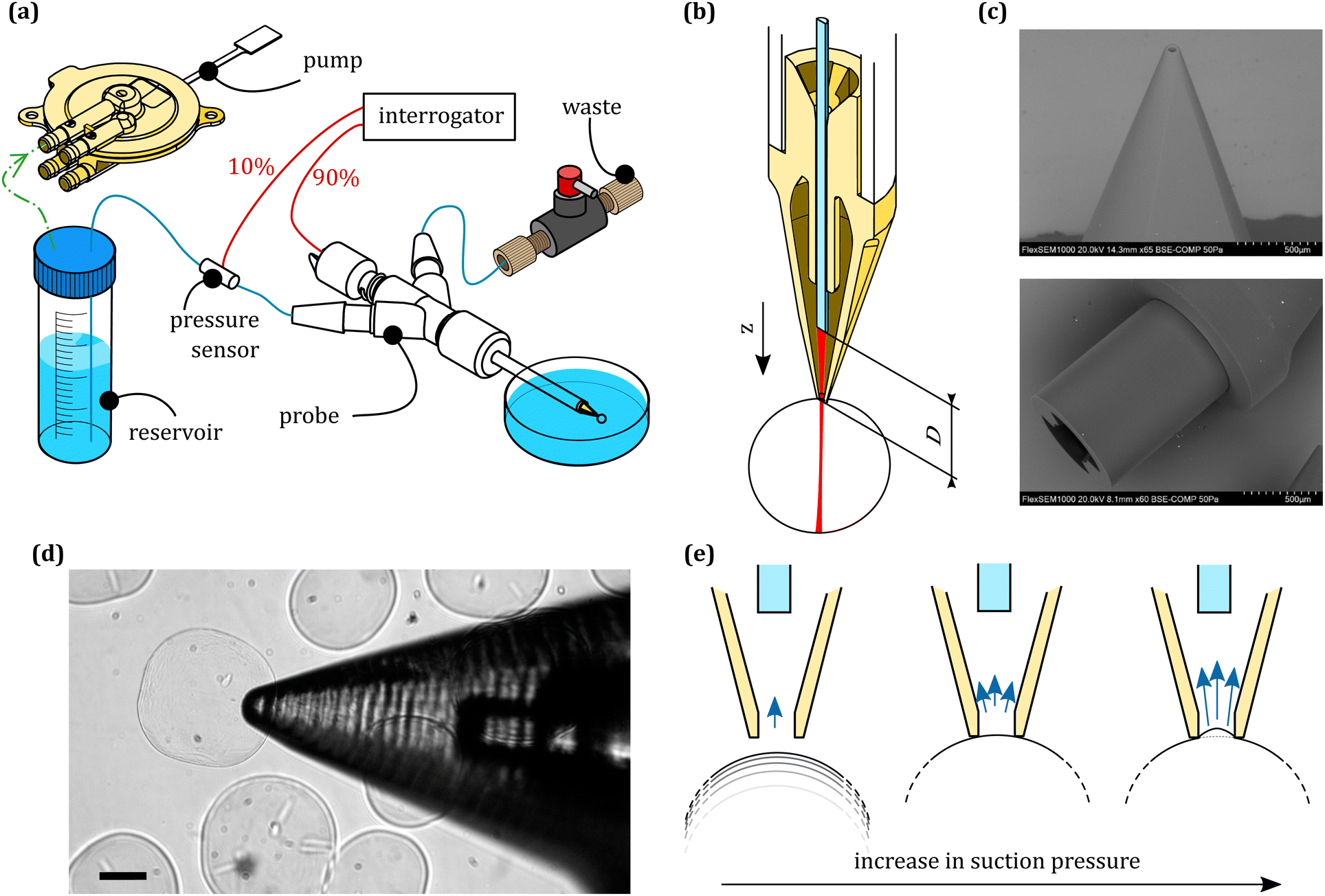 | ||
| Fig. 1 Hydraulic force spectroscopy (HFS) system. (a) Schematic depiction of the components. A piezoelectric micropump is connected to the water reservoir (green line), and applies a partial vacuum inside it. A second tube (blue line) connects the bottom of the reservoir with the probe. Alongside it, a T-shaped junction houses the optical pressure sensor. Both the probe and pressure sensor are connected to the fiber optic interrogator via an asymmetric splitter (red lines). (b) Schematic cross-section of the 2PP tip, highlighting the suspended internal ferrule for guiding the microlensed fiber. D is the fiber to sample distance, whose phase is monitored to extract the aspirated length of the sample within the pipette. (c) Scanning electron microscopy pictures of the 2PP tip (courtesy of UpNano). (d) Brightfied image of an HFS experiment, showing the probe capturing a microbead. On the right side, within the tip, it is possible to see the end facet of the optical fiber. Scale bar: 100 μm. (e) Schematic depiction of the working principle of an HFS experiment. As the suction pressure (denoted by the blue arrows) is increased, a sample is drawn to the pipette tip. As it makes contact with the pipette wall, it starts creeping in. | ||
The optical interrogator including a polychromatic source (1550 nm of center wavelength and 50 nm of FWHM) is connected to a depolarizer and a circulator. From the circulator, light travels through a 2 × 1 90![[thin space (1/6-em)]](https://www.rsc.org/images/entities/char_2009.gif) :10 wideband splitter that delivers the light to the displacement and the pressure sensors, respectively. The light is then collected and measured by a spectrometer connected to the circulator output. The two sensors are both fiber-based, with the displacement sensor being a microlensed fiber, and the pressure sensor a cleaved single mode fiber with a flexible MEMS membrane glued on top. A more detailed breakdown of the components is available in our previous work.18
:10 wideband splitter that delivers the light to the displacement and the pressure sensors, respectively. The light is then collected and measured by a spectrometer connected to the circulator output. The two sensors are both fiber-based, with the displacement sensor being a microlensed fiber, and the pressure sensor a cleaved single mode fiber with a flexible MEMS membrane glued on top. A more detailed breakdown of the components is available in our previous work.18
The hydraulic part has a water reservoir, connected to a piezoacoustic pump (TTP Ventus). This consists of a piezoelectic membrane that oscillates in a chamber, generating nodes and antinodes in correspondence with flapping valves, which allow us to depressurize the water reservoir following arbitrary profiles in time. Because of the rapid response time of the membrane, we were able to achieve a closed loop operation in pressure control with a frequency range of 0.01–30 Hz.
The probe has a 3D printed housing that contains the sensors and a zirconia sleeve that ensures alignment between a capillary and the displacement detection fiber. At the back, it has barbed connectors to deliver fluid to the capillary tip. The housing is composed of three parts; a main body, where the capillary and the sensors are inserted, a screw cap with an o-ring that is used to fix the capillary in place and allows for rapid substitution, and a second screw insert where the displacement sensor is glued. This is used to adjust the fiber to the sample distance. The 3D printed components were manufactured via stereolitography (Form 2, Formlabs), using clear resin (v4, Formlabs). Contrary to the standard procedure in micropipette aspiration, the aspiration nozzle was manufactured via 2 photon polymerization (2PP) 3D printing. This process allowed printing a monolithic structure that features both the aspiration aperture (50 μm diameter) and the suspended fiber guide, which optimized the fiber/nozzle alignment and thereby maximized the light collection from the sample. The nozzles were printed by UpNano GmbH, using UpPhoto material and a 10× objective. The nozzle was glued to a glass capillary using UV-curing adhesive (NOA61, Thorlabs).
HFS works by measuring the phase variation between the light reflecting off the fiber end facets and the light that reflects either off the sample or the MEMS membrane, detected by sensor optical cavities. By using a polychromatic source and controlling the fiber to reflector distance, it is possible to multiplex sensors and analyze their behavior in time independently. This is done by taking the Fourier transform of the measured signal and extracting the phase of its local maxima. The displacement is retrieved using:
 | (1) |
 is the mean wavelength of the source, and n is the refractive index of the medium between the fiber and the reflective surface (n = 1 for the cavity associated with the pressure sensor, n = 1.33 for the one associated with the displacement sensor). The pressure sensor is calibrated by measuring the phase variation equivalent to a known vertical displacement of the water reservoir (kp = 76.59 Pa nm−1).
2.3 Mechanical testing protocol
To characterize the hydrogels with the HFS system, we mounted 50 μm diameter nozzles on the probe. After capturing a bead by applying a faint pressure of 20 Pa, we applied a linear ramp on the aspiration pressure, reaching ≈500 Pa after 5 seconds, followed by a holding period of 30–40 seconds. After that, we performed a sequence of 2–20, ≈50 Pa oscillations between 0.05 Hz and 20 Hz, separated by 2 seconds each. After that, we released the sample and repeated the same procedure on different microbeads.We performed the nanoindentation experiments with an AFM Nanowizard IV (JPK Instruments – Bruker) using spherical tip cantilevers (CP-PNPS-BSG-C, and CP-PNPL-SiO-B, NanoAndMore) with a 0.32 N m−1 spring constant. The spherical probes had a 3.5 or 20 μm diameter. We coated Petri dishes with poly-L-lysine (0.01% for 30 minutes) before placing the microbeads to avoid movement during indentation. An indentation ramp up to 300–600 nm was applied depending on the cantilever and followed by a 30 s holding phase at the same depth, during which stress relaxation occurred. After that, we performed the dynamic characterization at 9 logarithmically spaced frequencies between 0.25 and 150 Hz, oscillating with an amplitude of 60 nm for a minimum of 5 periods per frequency and with 2 seconds of rest in between frequencies. Lastly, we retracted the cantilever with symmetric unloading. We measured only the central portion of each trapped hydrogel to minimize variability that would arise from non-Hertzian contact or uncontrolled rotations of the sample.
We performed both experiments in deionized water, collecting data from 30 different microbeads for both AFM and HFS. In the case of AFM, we collected 2 × 2 force maps on each microbead and averaged the resulting values.
3 Modeling
3.1 Hydrodynamic drag correction for HFS
When dealing with a fluid in motion, it is important to verify the role of inertial and viscous forces to avoid erroneous estimation of the applied pressure and loss factor.20 To this end, the Womersley number can be used to gauge the extent to which the inertial forces are relevant with respect to the viscous forces.21 It is defined as: | (2) |
 | (3) |
| δHD(ω) = arctan(ℑ(P*)/ℜ(P*)) | (4) |
 | ||
| Fig. 2 Experimental measurement of the hydrodynamic drag effect. (a) Schematic representation of the experimental setup, highlighting the pipes’ dimensions and the distance between the sensors. (b) Unfiltered, unwrapped phase from the pressure sensors. Increasing flow velocity has a negligible impact on the amplitude of the pressure oscillation at the tip. (c) Frequency dependent response of the system. On the left axis is the complex pressure response as a function of the actuation frequency. The two black lines represent the in (o) and out (*) of phase terms. At low frequencies, the pressure at the tip lags the measurement done in the tube by a few μs. As the actuation frequency increases, the lag increases to a few ms at 25 Hz, corresponding to a phase lag of approximately 10 degrees. The right axis shows the phase lag, calculated using eqn (4). | ||
The best fit for the phase lag is shown in Fig. 2(c), on the right y-axis. The fitting equation is:
| δHD(ω) = arctan(A·ωB) | (5) |
3.2 HFS modeling
We modeled the HFS data using the approach we proposed in our previous work.18 Starting from the constitutive equation derived by Zhou et al.,24 we neglect the shape correction terms of order 2 and higher, as the imposed deformation is very small compared to the size of the sample. This results in a linearized form:9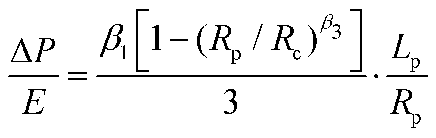 | (6) |

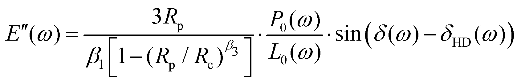 | (7) |
3.3 AFM modeling
The AFM data was modeled using Hertzian contact theory, calculating E′ and E′′ as:25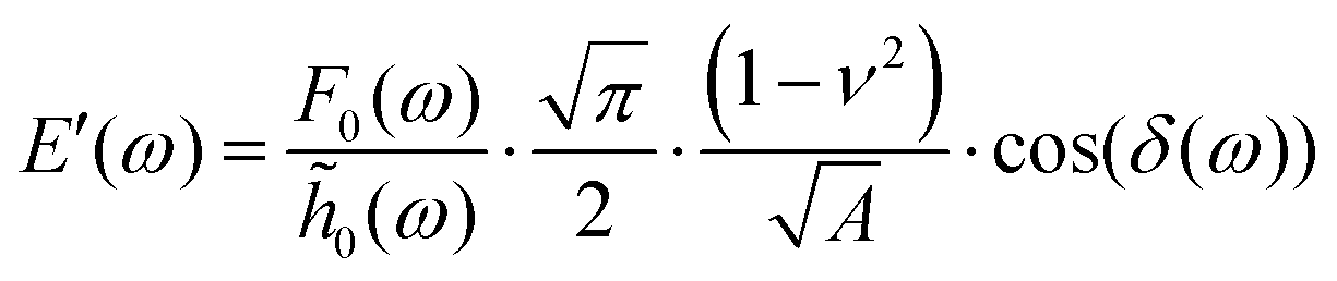
 | (8) |
![[h with combining tilde]](https://www.rsc.org/images/entities/i_char_0068_0303.gif) 0 are the load and indentation amplitudes of the oscillation respectively, ν is the Poisson ratio (assumed to be 0.5), Ri is the probe radius, and δ is the phase lag between load and indentation, and A is the contact area.
0 are the load and indentation amplitudes of the oscillation respectively, ν is the Poisson ratio (assumed to be 0.5), Ri is the probe radius, and δ is the phase lag between load and indentation, and A is the contact area.
Since the nanoindentation modeling relies on the Hertzian theory, the reliability of the extracted mechanical properties depends on how well the experimental setup complies with the theoretical assumptions. The previous work of Glaubitz et al.26 showed that the modeling spherical particles indented by spherical probes requires a corrected version of the Hertz's model, since this would predict larger contact areas and neglects the sphere/substrate small area of contact and associated deformation. In this case, the mass density of the microbead is barely above that of its surroundings and its elastic modulus is relatively high. This implies that the sample to substrate contact is small, comparable to that of the sample to probe, and therefore the microbead does not collapse under its own weight. Given a spherical probe, a spherical sample, and a flat substrate, the correction factor for the indentation is:
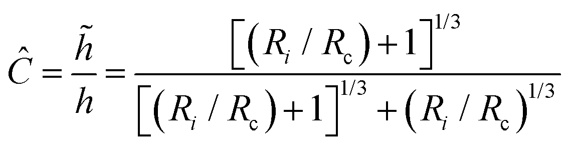 | (9) |
Ri.
Note that we did not apply hydrodynamic drag correction to these curves, as the effect is minimal for the given frequency range under study and the cantilever-substrate distance.20 Similarly, we neglected the effects of probe-sample adhesive contact that are considered in alternative nanoindentation modeling approaches, such as JKR.27 Observing the experimental AFM curves (see the ESI,† Fig. S1), it appears clear that adhesive effects play a very small role. Typically, the adhesion force measured around 3% of the maximum applied load.
3.4 Finite elements analysis
We simulated both aspiration and indentation of hydrogel microspheres using ANSYS Mechanical APDL 2021-R2 (ANSYS Inc.). We modeled both conditions as 2D axisymmetric contact problems, where the contact surfaces (pipette walls, indenter, and substrate) are rigid and approximately frictionless.We assumed that the hydrogel material to be isotropic and homogeneous, and performed simulations for both linear viscoelastic and poroelastic constitutive behaviors. In the case of indentation, we simulated both the condition of a sphere on a substrate being indented and a half sphere rigidly connected to a substrate. The second condition was obtained starting from the first simulation, imposing a zero displacement boundary condition on all the nodes below the circumference.
We defined mapped meshes with densification in correspondence of the contact regions (see Fig. 3), and ran a mesh sensitivity analysis to optimize the number of elements and computation time. Each model consisted of ≈5000 eight node elements with a mixed u-P formulation.
 | ||
| Fig. 3 FE mesh for HFS (left) and AFM (right) simulations, with a highlight on the contact surfaces, i.e. the pipette wall on the left, and the indenting sphere and substrate on the right. The arrows represent the loading applied on the sample: distributed line pressure for HFS, force on the indenter for AFM. | ||
4 Results and discussion
As shown in Fig. 2, the hydrodynamic drag correction is fundamental for estimating the correct phase lag between pressure and displacement of the sample, at least for the frequencies above 1 Hz. The dependency of the lag on the frequency appears more severe than what the Womersley number would estimate (ω0.9vs. ω0.5), which may be related to the changes in channel shape and flow characteristics. In the nozzle, the channel is initially ring shaped (because of the presence of the sensing fiber), before switching to a tapered cylinder until the orifice, which is a short straight cylinder. On the other hand, the amplitude of the signal seems unaffected.Fig. 4 shows a typical measurement obtained using the HFS method and Fig. 5(a) shows the complex modulus measured with both the AFM and HFS systems, as mean ± SD. Since the nanoindentation results are notoriously affected by the contact size,28–30 we first compared the HFS microrheology with the AFM results obtained with the 20 μm bead. This is because the latter set of experiments has a characteristic experimental length (i.e. the contact radius) that is as close as we could get to that of HFS. We chose the test parameter such that both experiments would lead to a deformation of ≈5%, in order to be comparable with one another and fulfill the small strain approximation.
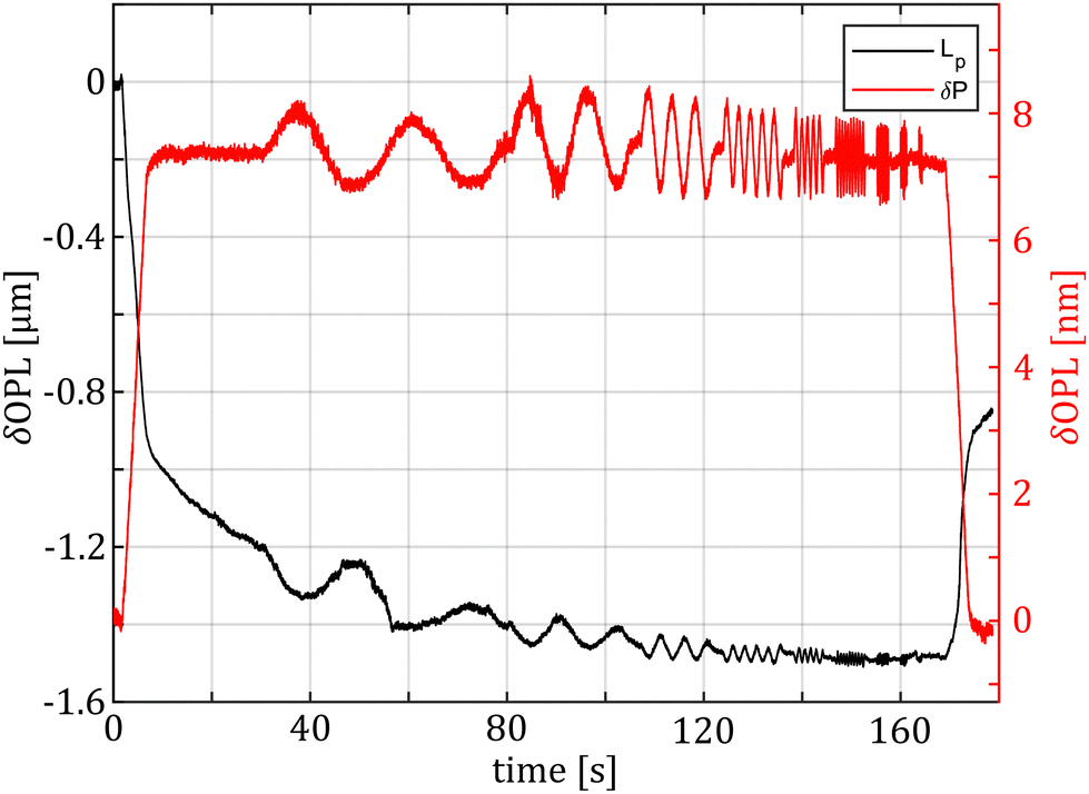 | ||
| Fig. 4 Example of unwrapped phase data obtained from an aspiration experiment. Pressure variation (red) and aspirated length (black) are in opposition as they share the same frame of reference, that considers positive variations as the fiber to the reflection cavity increases. The pressure sensor shows a linear ramp that stops at 7 nm of displacement, corresponding to ≈500 Pa. Note that the optical path length variation (δOPL) of the aspirated length needs to be divided by 1.33 (i.e. the refractive index of water) to obtain the actual geometrical value d. | ||
 | ||
| Fig. 5 Dynamic analysis of alginate microbeads. Note that the HFS data points have been shifted (≈10% downward) with respect to the actual measurement frequency to improve clarity and avoid overlapping error bars. Solid and dashed lines are linear interpolations between data points. (a) Frequency dependent response as measured by the HFS (blue) and AFM (gold) systems, displayed as mean ± SD (N = 30). The two methods capture very similar behaviors, with comparable E* magnitude. Both storage and loss moduli monotonically increase between 0.25 and 20 Hz, with comparable trends between AFM and HFS. (b) The tanδ estimated at the 6 common frequencies, displayed as mean ± SD (N = 30). HFS systematically estimates lower viscous losses, with a phase lag difference of ≈8 degrees with respect to AFM. | ||
Both methods appear to capture the same trends in storage and loss moduli, which monotonically increase between 0.01 and 20 Hz. Over the 3 partly overlapping decades, the storage modulus obtained with the HFS and AFM systems almost doubles and the loss modulus increases approximately 3.5 fold. Although the storage modulus estimation seems to be the same, there is a clear gap between the loss moduli at all overlapping frequencies. Plotting the loss factor (defined as tanδ = E′′/E′) vs. the measurement frequency reveals a ≈0.15 gap between the measured means. This discrepancy appears to be approximately independent of the frequency, hinting at a systematic measurement bias.
Considering that the pre-stress leads to similar strain values for both techniques and the oscillation amplitude was less than 100 nm in both cases, we concluded that it is unlikely to link such differences to material nonlinearity.
HFS consistently estimates lower viscous losses. This method encodes both the pressure and displacement information in the same interferometric signal making them naturally synchronized, so we can exclude that the discrepancy is associated to timing/data acquisition issues. We first hypothesized that the AFM method may suffer from limitations in the measurement protocol: practically, it is difficult to position the probe exactly above the sample-to-substrate contact point, especially if the microsphere is not perfectly spherical. This would result in measurements where the sample is also moving, and this additional compliance is not accounted for by the model. As the force maps were collected at the apex of the microspheres, assuming that off-center measurements would suffer from additional purely dissipative effects, we hypothesized that the AFM tanδ distribution would feature one “true” peak related to the material behavior and a second peak resulting from the ill-conditioned measurements. However, the tanδ distributions obtained with the AFM and HFS systems at six common frequencies (Fig. 6) do not support this hypothesis because the AFM results (here referring to single, non-pooled indentation curves) do not feature modes that are overlapping with the HFS results.
 | ||
| Fig. 6 Comparison of the kernel density estimated in the HFS (N = 30) and AFM (N = 120) systems at all overlapping frequencies. Both methods seem to have only one dominant mode, with a relatively constant distance between them (approximately 0.15). It is worth noting that AFM results yield, in a few cases, very high tanδ values, up to ≈1.5. Looking at the associated force-distance curves, it appears that gliding or detachment occurred in such cases. However, the rarity of such events make it unlikely that the discrepancy between the two loss factors is associated with such phenomena. | ||
We then moved to FEM to assess the influence of boundary conditions and the validity of the models we chose to obtain E*. First, we analyzed whether the modeling choices we made for AFM were appropriate for this experimental configuration. In particular, we verified the validity of the Glaubitz model for dynamic indentation. Whilst this correction (eqn (9)) was obtained for linear elastic bodies, the simulation results confirmed that it still holds up in the viscoelastic case (see Fig. 7). Since the force and pressure oscillations cause tens of nanometers of displacement and the contact conditions do not change meaningfully during the dynamic analysis, we can assume that the complex modulus estimation is accurate. The simulation results confirmed this hypothesis since we were able to extract the same material parameters from the force/displacements curves of both the HFS and AFM simulations using eqn (6) and (7).
 | ||
| Fig. 7 Comparison of the AFM FE simulation for the indentation on a full sphere (free) and a half sphere (bound). The first two data sets are the result of sinusoidal oscillation on the same material, keeping both frequency and load amplitude constant, and changing the boundary conditions. In the full sphere case, the indentation cannot be simply measured as the difference between cantilever deflection and piezo movement, as this ignores the sample/substrate contact compliance and overestimates the actual indentation. By using eqn (9), the results match with the half sphere case (corrected). | ||
Assuming the boundary conditions are reasonably captured by our model, we investigated scale-dependent material behavior as a possible source of discrepancy. In particular, we hypothesized our sample would feature both viscoelastic and poroelastic relaxation. Therefore, we investigated poroelastic effects as a possible source of discrepancy via FEM. Poroelasticity31 is a scale dependent property, whose characteristic relaxation time, τ, scales with the square of the characteristic length of the experiment a:
| τ = a2/D | (10) |
 , i.e. the indentation contact radius from the indentation depth, and as aHFS = Rp, i.e. the pipette radius.31,32 The diffusivity of ionically crosslinked alginate hydrogels has been reported to be between 10−9 to 10−11 [m2 s−1],32 depending on the synthesis procedure. For the AFM measurements, this would translate to a relaxation frequency that peaks between ≈2 and 200 Hz, which falls in the experimental range under investigation. For the HFS measurements, owing to the significantly larger a, 1/τ would lie between ≈0.02 and 2 Hz. That being said, this estimate is not necessarily reliable, as the two conditions are quite different. In the nanoindentation measurements, the structure is drained as the porosity collapses and the probe is impermeable, whereas in the HFS measurements the strain has mostly a positive sign and water is free to flow at the sample interface. There is some evidence in the literature hinting at an asymmetric behavior between tension and compression: previous studies found that the relaxation times of fibrous samples under tension were notably shorter than those under compression.33–35 However, to the best of our knowledge, there are no studies that analyze the poroelastic effects under aspiration.
To clarify the possible differences between the two loading modes, we simulated a number of creep experiments (see the inset, Fig. 8), with varying pipette and indenter radii. In all cases, we kept the same sample material properties. The results are shown in Fig. 8. As expected, when plotting the normalized load versus time, every simulation follows a different path. However, when we normalize the time to that of poroelastic relaxation, the simulations do not overlap, but instead collapse on two distinct curves, which represent the two different experiments.
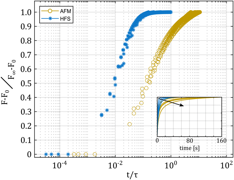 | ||
| Fig. 8 Results of poroelastic creep FE models for the HFS and AFM measurements. The plot shows the normalized force vs. time, normalized to the characteristic poroelastic time τ. The inset shows the normalized creep versus time for the studied conditions. We varied the pipette radius between 10 and 50 μm, and the AFM contact radius between 1 and 5 μm. The arrow in the inset indicates increasing radii, for both AFM and HFS. As the contact area increases, the time required to reach equilibrium also increases. Although HFS has a significantly larger characteristic area than AFM in all of the simulations, it always reaches equilibrium faster. | ||
The indentation curve qualitatively follows the same behavior that was demonstrated in a previous work on the poroelasticity of microbeads.2 On the other hand, the aspiration simulations, while all overlapping when normalized to t/τ, appear to reach equilibrium much faster than expected, despite the much larger deformed surface of the HFS experiment. Since the value of tanδ measured with the HFS system is systematically lower than the one obtained with the AFM system, it is possible that the discrepancy comes from a combined viscoelastic behavior plus an incomplete poroelastic relaxation in the AFM results.31
Unfortunately, as the characteristic length of HFS is the pipette radius, the finite size of the microbead does not allow increasing the contact surface sufficiently to bring the poroelastic effect in the probed range. On the other hand, by reducing the contact radius in AFM, we can push the poroelastic effects toward higher frequencies.31
On the basis of the FE findings, we repeated the indentation experiments using smaller contact surfaces, as the smaller the characteristic length, the higher the characteristic poroelastic frequency. Using a spherical probe with 3.5 μm diameter, we obtained sub-μm contact radii, which shift the possible poroelastic peak between 80 and 8000 Hz. E* calculations yield similar curves (see the ESI,† Fig. S2), but translated toward higher values (approximately 3× for the storage modulus and 2× for the loss modulus). In this second set of indentation experiments, the imposed deformation was still compatible with the small strain approximation, making it unlikely that the difference was tied to a material nonlinearity.36 This scale stiffening effect is well documented in the literature, albeit not fully explained.28–30 Previous studies on hydrogels observed an increase in the estimated stiffness with decreasing contact areas.37–39 Micropipette aspiration, and by extension HFS, are approximately indifferent to the sample/pipette contact conditions, as the area subject to pressure is constant. By contrast, AFM is very sensitive to the definition of the contact point, as the contact area is tied to the indentation.40 Erroneous estimates could lead to up to 10-fold variation in the estimation of the elastic modulus.41 This being said, in our experiments the signal to noise ratio is very good (see the ESI,† Fig. S1), so we assumed such errors to be limited. We hypothesized that in this case, the discrepancy could be related to the porous nature of the sample: whilst the material is essentially a trabecular structure filled with water, the mechanical model we employed for its characterization is assumed to be continuous. This means that as the volume that is averaged in each measurement approaches the scale of the porosity, the contribution of the load bearing portion (i.e. the polymer fraction) changes. Previous works linked the scale of investigation to different constituents of hydrogels, noting how reducing the scale of investigation leads to a shift towards= the characterization of the fibrous network of the gel39 instead of its bulk response.
We assumed that, even if at the sub-μm scale the nominal contact area is not actually a scaled version of what we observe with HFS or larger AFM probes, and we can still make use of tanδ to compare measurements. This is because the loss factor simply quantifies how much energy per cycle is lost in the material due to dissipative phenomena, and its definition does not depend on the quantification of a contact area.
As shown in Fig. 9, a smaller contact area does indeed lead to lower tanδ values. More importantly, the low frequency tanδ plateau matches well with the results obtained with the HFS system. Since the poroelastic effect has a characteristic frequency at which energy dissipation is maximized,31 and this frequency is an extrinsic property, the contact area reduction “moves” the poroelasticity effect toward higher frequencies, outside our probed range. This allows us to measure the intrinsic viscoelastic properties. The agreement we found supports the hypothesis that the first set of AFM results appear different because of the superposition of different dissipative phenomena.
 | ||
| Fig. 9 Comparison of the tanδ values obtained with the HFS and the AFM (using a 3.5 μm diameter tip) systems. By reducing the contact area, the characteristic poroelastic relaxation time is pushed toward higher frequencies, outside of the overlapping testing window. With only the viscoelastic response contributing to the viscous losses, AFM and HFS estimate the same tanδ. Note that the HFS data points have been shifted (≈10% downward) with respect to the actual measurement frequency to improve clarity and avoid overlapping error bars. The results are displayed as mean ± SD. The dashed grey data are the tanδ values obtained with the larger 20 μm diameter tip, for which poroelastic effects are present and compound with the viscous losses. | ||
5 Conclusions
We have shown how hydraulic force spectroscopy can be applied to study the rheological properties of soft, suspended bodies over several decades. Experimental results, paired with FE simulations, showed that (1) acknowledging and quantifying the sample to substrate contact is crucial to obtain accurate viscoelasticity values via nanoindentation, (2) the contact correction previously reported for elastic problems also applies to the viscoelastic case and (3) the poroelastic effects are asymmetric in indentation and aspiration. In this case, the material showed a predominantly viscoelastic behavior, compatible with previous literature reports.17 Our experimental results showed that both methods provide a viable solution for characterization of soft suspended bodies, with a level of agreement that is qualitatively similar to other studies that compared commercial devices for dynamic mechanical analysis.42,43 Our results, whilst not obtained on biological samples, have interesting implications for studies on cell mechanics. The diffusivity of cells and their constituents has been reported44,45 to be in the order of 10−12–10−14 [m2 s−1]. It is reasonable to assume that in the testing range of 0.01–100 [Hz] the poroelastic effects can be neglected at the common scales of investigation probed with instruments such as AFM, MPA, and micro-tweezers. This implies that discrepancies in the estimation of mechanical properties are not necessarily a problem of calibration and ill-conditioned models, but could arise from how the material is structured and its non-affine deformations.Thanks to the simplified modeling and workflow, the HFS system is a valuable addition to the toolkit of materials scientists. Considering the previously reported discrepancies between AFM and MPA, we demonstrated a reliable, repeatable and highly sensitive system that can uncover exciting applications in the fields of materials science and soft matter mechanics.
Author contributions
M.B.: conceptualization, methodology, hardware, software, visualization, original draft, formal analysis, investigation, and writing – review and editing. M. B., K. G.: formal analysis, investigation, and writing – review and editing. M. B., K. G. and J. J.: investigation, and writing – review and editing. C. W. V., M. L. and B. I. A.: writing - review and editing.Conflicts of interest
M. B. and K. B. are employed at Optics11 B. V., C. V. W. is the co-founder and CSO of IamFluidics B. V., Optics11 B. V. applied for a patent covering some aspects of the HFS apparatus.Acknowledgements
This work was financially supported by the H2020 European Research and Innovation Programme under the Marie Skłodowska-Curie grant agreement “Phys2BioMed” contract no. 812772.Notes and references
- A. Sakai, Y. Murayama and M. Yanagisawa, Langmuir, 2020, 36, 5186–5191 CrossRef CAS PubMed
.
- J. D. Berry, M. Biviano and R. R. Dagastine, Soft Matter, 2020, 16, 5314–5324 RSC
- N. Isobe, S. Kimura, M. Wada and S. Deguchi, J. Taiwan Inst. Chem. Eng., 2018, 92, 118–122 CrossRef CAS
- P. H. Wu, D. R. B. Aroush, A. Asnacios, W. C. Chen, M. E. Dokukin, B. L. Doss, P. Durand-Smet, A. Ekpenyong, J. Guck, N. V. Guz, P. A. Janmey, J. S. Lee, N. M. Moore, A. Ott, Y. C. Poh, R. Ros, M. Sander, I. Sokolov, J. R. Staunton, N. Wang, G. Whyte and D. Wirtz, Nat. Methods, 2018, 15, 491–498 CrossRef CAS PubMed
- C. J. McCarthy, C. Birkinshaw, J. T. Pembroke and M. Hale, Biotechnol. Tech., 1991, 5, 493–496 CrossRef
- X. Li and J. P. Gong, Proc. Natl. Acad. Sci. U. S. A., 2022, 119, 1–8 Search PubMed
-
J. Bergström, Mechanics of Solid Polymers: Theory and Computational Modeling, 2015, pp. 1–509 Search PubMed
- L. Z. Yanez, J. Han, B. B. Behr, R. A. Pera and D. B. Camarillo, Nat. Commun., 2016, 7, 1–12 Search PubMed
-
B. González-Bermúdez, G. V. Guinea and G. R. Plaza, Advances in Micropipette Aspiration: Applications in Cell Biomechanics, Models, and Extended Studies, 2019 Search PubMed
- H. D. Ou-Yang and M. T. Wei, Annu. Rev. Phys. Chem., 2010, 61, 421–440 CrossRef CAS PubMed
- A. C. Hodgson, C. M. Verstreken, C. L. Fisher, U. F. Keyser, S. Pagliara and K. J. Chalut, Lab Chip, 2017, 17, 805–813 RSC
- M. H. Panhwar, F. Czerwinski, V. A. Dabbiru, Y. Komaragiri, B. Fregin, D. Biedenweg, P. Nestler, R. H. Pires and O. Otto, Nat. Commun., 2020, 11, 1–13 CrossRef
- R. Daza, B. González-Bermúdez, J. Cruces, M. De la Fuente, G. R. Plaza, M. Arroyo-Hernández, M. Elices, J. Pérez-Rigueiro and G. V. Guinea, J. Mech. Behav. Biomed. Mater., 2019, 95, 103–115 CrossRef CAS
- C. M. Buffinton, K. J. Tong, R. A. Blaho, E. M. Buffinton and D. M. Ebenstein, J. Mech. Behav. Biomed. Mater., 2015, 367–379 CrossRef CAS
- H. Van Hoorn, N. A. Kurniawan, G. H. Koenderink and D. Iannuzzi, Soft Matter, 2016, 12, 3066–3073 RSC
- A. Stracuzzi, B. R. Britt, E. Mazza and A. E. Ehret, Biomech. Model. Mechanobiol., 2022, 21, 433–454 CrossRef PubMed
- V. B. Nguyen, C. X. Wang, C. R. Thomas and Z. Zhang, Chem. Eng. Sci., 2009, 64, 821–829 CrossRef CAS
- M. Berardi, K. Bielawski, N. Rijnveld, G. Gruca, H. Aardema, L. van Tol, G. Wuite and B. I. Akca, Commun. Biol., 2021, 4, 610 CrossRef CAS PubMed
- C. W. Visser, T. Kamperman, L. P. Karbaat, D. Lohse and M. Karperien, Sci. Adv., 2018, 4, 1–9 Search PubMed
- J. Alcaraz, L. Buscemi, M. Puig-De-Morales, J. Colchero, A. Baró and D. Navajas, Langmuir, 2002, 18, 716–721 CrossRef CAS
- J. R. Womersley, J. Physiol., 1955, 127, 553–563 CrossRef CAS
- S. Uchida, Z. Angew. Math. Phys., 1956, 7, 403–422 CrossRef
- A. Siginer, Int. J. Eng. Sci., 1991, 29, 1557–1567 CrossRef CAS
- E. H. Zhou, C. T. Lim and S. T. Quek, Mech. Adv. Mater. Struct., 2005, 12, 501–512 CrossRef
- E. G. Herbert, W. C. Oliver and G. M. Pharr, J. Phys. D: Appl. Phys., 2008, 41, 074021 CrossRef
- M. Glaubitz, N. Medvedev, D. Pussak, L. Hartmann, S. Schmidt, C. A. Helm and M. Delcea, Soft Matter, 2014, 10, 6732–6741 RSC
- M. Ciavarella, J. Joe, A. Papangelo and J. R. Barber, J. R. Soc., Interface, 2019, 16, 20180738 CrossRef CAS
- C. S. Han and S. Nikolov, J. Mater. Res., 2007, 22, 1662–1672 CrossRef CAS
- C. S. Han, Mater. Sci. Eng. A, 2010, 527, 619–624 CrossRef
- C. S. Han, S. H. Sanei and F. Alisafaei, J. Polym. Eng., 2016, 36, 103–111 CrossRef
- Y. Lai and Y. Hu, Soft Matter, 2017, 13, 852–861 RSC
- Y. Hu and Z. Suo, Acta Mech. Solida Sin., 2012, 25, 441–458 CrossRef
- D. G. Strange, T. L. Fletcher, K. Tonsomboon, H. Brawn, X. Zhao and M. L. Oyen, Appl. Phys. Lett., 2013, 102, 1–5 CrossRef
- D. G. Strange, K. Tonsomboon and M. L. Oyen, J. Mater. Sci.: Mater. Med., 2014, 25, 681–690 CrossRef CAS
- M. A. Soltz and G. A. Ateshian, J. Biomech. Eng., 2000, 122, 576–586 CrossRef CAS PubMed
- D. C. Lin, D. I. Shreiber, E. K. Dimitriadis and F. Horkay, Biomech. Model. Mechanobiol., 2009, 8, 345–358 CrossRef PubMed
- S. Huth, S. Sindt and C. Selhuber-Unkel, PLoS One, 2019, 14, 1–17 CrossRef
- J. Zemła, J. Bobrowska, A. Kubiak, T. Zieliński, J. Pabijan, K. Pogoda, P. Bobrowski and M. Lekka, Eur. Biophys. J., 2020, 49, 485–495 CrossRef
- R. Akhtar, E. R. Draper, D. J. Adams and J. Hay, J. Mater. Res., 2018, 33, 873–883 CrossRef CAS
- L. Puricelli, M. Galluzzi, C. Schulte, A. Podestà and P. Milani, Rev. Sci. Instrum., 2015, 86, 033705 CrossRef PubMed
- N. Gavara, Sci. Rep., 2016, 6, 21267 CrossRef CAS PubMed
- R. Hagen, L. Salmén, H. Lavebratt and B. Stenberg, Polym. Test., 1994, 13, 113–128 CrossRef CAS
- I. R. Henriques, L. A. Borges, M. F. Costa, B. G. Soares and D. A. Castello, Polym. Test., 2018, 72, 394–406 CrossRef CAS
- E. Moeendarbary, L. Valon, M. Fritzsche, A. R. Harris, D. A. Moulding, A. J. Thrasher, E. Stride, L. Mahadevan and G. T. Charras, Nat. Mater., 2013, 12, 253–261 CrossRef CAS
- S. T. Johnston, E. T. Shah, L. K. Chopin, D. L. S. McElwain and M. J. Simpson, BMC Syst. Biol., 2015, 9, 38 CrossRef
Footnote |
| † Electronic supplementary information (ESI) available: Fig. 1 example of an AFM indentation curve. Fig. 2 complex modulus vs. frequency response from AFM dynamic nanoindentation. See DOI: https://doi.org/10.1039/d2sm01173e |
| This journal is © The Royal Society of Chemistry 2023 |