Determination of protein conformation and orientation at buried solid/liquid interfaces

Abstract

Protein structures at solid/liquid interfaces mediate interfacial protein functions, which are important for many applications. It is difficult to probe interfacial protein structures at buried solid/liquid interfaces in situ at the molecular level. Here, a systematic methodology to determine protein molecular structures (orientation and conformation) at buried solid/liquid interfaces in situ was successfully developed with a combined approach using a nonlinear optical spectroscopic technique – sum frequency generation (SFG) vibrational spectroscopy, isotope labeling, spectra calculation, and computer simulation. With this approach, molecular structures of protein GB1 and its mutant (with two amino acids mutated) were investigated at the polymer/solution interface. Markedly different orientations and similar (but not identical) conformations of the wild-type protein GB1 and its mutant at the interface were detected, due to the varied molecular interfacial interactions. This systematic strategy is general and can be widely used to elucidate protein structures at buried interfaces in situ.

---

Introduction

Interfacial protein activities play important roles in a broad range of applications, such as biomedical implants, marine anti-biofouling coatings, biosensors, membrane protein functions, and antibody drug storage and administration.^1–7 It is well known that protein structures determine their functions. Therefore, it is important to understand molecular structures of proteins at interfaces to optimize their interfacial interactions and to improve their interfacial functions. Excellent progress has been made to understand protein structures in bulk environments using X-ray diffraction and NMR, but it is difficult to determine protein structures at interfaces in situ. Atomic force microscopy (AFM)⁸ maps interfacial morphologies of proteins, but has the potential to perturb its targets and makes it difficult to examine detailed molecular conformations. Surface plasmon resonance (SPR)⁹ can follow the kinetics of their interfacial adsorption behavior, but cannot provide molecular level signatures of these biological molecules. Attenuated total reflection Fourier transform infrared spectroscopy (ATR-FTIR)¹⁰ and surface-enhanced Raman spectroscopy (SERS)¹¹ have been applied to obtain molecular level vibrational fingerprints of interfacial proteins. However, ATR-FTIR suffers from water interference and inadequate surface sensitivity. Sample preparation for SERS could be complicated, and the usage of a metallic surface may limit the general application of SERS to study proteins at different interfaces.

A technique with excellent surface sensitivity and in situ capability is required to study the molecular structures of interfacial proteins. Sum frequency generation (SFG) vibrational spectroscopy, a second-order nonlinear optical spectroscopy, is an appropriate technique to fulfill these requirements. As a vibrational spectroscopy, SFG inherits the advantages of ATR-FTIR and SERS, by being capable of recording molecular vibrational features.^12–30 The selection rules of SFG determine that it can only detect signals from a medium where inversion symmetry is broken under the electric dipole approximation, making SFG intrinsically surface/interface specific with a sub-monolayer sensitivity.^12–30 The non-invasive nature of SFG allows in situ observation of structural changes in interfacial proteins. In addition, SFG can probe interfacial molecular orientation by applying different polarization combinations, allowing in-depth analysis of protein molecular behavior and molecular interaction at interfaces. With these advantages, SFG has been developed into a powerful tool to probe interfacial structures of proteins in the last 20 years.^21,31–42

It has been demonstrated that isotope-labeling biological samples especially site-selective isotope labeling could greatly facilitate the elucidation of the structures of biomolecules using various experimental techniques, such as NMR, mass spectrometry, and vibrational spectroscopies.^43–45 Isotope labeling provides many advantages. For example, it could distinguish originally overlapping signals. Specifically for a vibrational spectroscopic technique, isotopic substitution of ¹³C in the backbone of proteins could shift the amide I band by ∼40 cm⁻¹.^46,47 Thus, isotope labeling generates many more independent spectral measurements, aiding in the determination of complex structures of biological molecules. In the current study, we combined the isotope labeling method with SFG spectroscopy to study interfacial behavior of the B1 domain of protein G (GB1).

GB1 is a small protein of 56 residues, forming two anti-parallel β-sheet structures near each terminus and an α-helix structure in the middle. The small size and rich secondary structure make GB1 an excellent model for many protein studies.^48–51 Previously, we studied the behavior of GB1 on a graphene surface and showed that residues Q32 and N35, located at the helical portion of GB1, play an important role in the strong protein–surface interaction with graphene, leading to the denaturation of the protein.⁵² The mutation of these two residues into alanine could greatly reduce the protein–graphene interaction and retain the native GB1 structure on graphene, preventing the denaturation of GB1.⁵² In the above study, we deduced the mutant GB1 orientation based on the GB1 crystal structure (PDB entry: 3gb1) and used the SFG signals from the α-helical domain in the orientation analysis.

Here in this study, we isotope labeled GB1 and its mutant, and developed a new systematic method to combine isotope labeling, SFG measurements, SFG Hamiltonian spectral simulation, and atomistic molecular dynamics (MD) simulation to determine the molecular structure of wild-type GB1 (WT GB1) and mutant GB1 Q32A and N35A (MT GB1) at the polymer/protein solution interface, using polystyrene (PS) as a polymer model. A one-exciton Hamiltonian approach was applied for SFG spectral construction of each protein structure as a function of protein orientation.^53–55 Atomistic MD simulations could describe the conformations of adsorbed proteins^56–58 and provide protein structure inputs for the Hamiltonian SFG spectral calculation program. The calculated spectra were compared to the experimental measurements to get matching scores. The highest matching score generated from the comparison considering all the isotope labeled proteins determines the most likely conformation (the input structure used) and orientation of WT GB1 or MT GB1 at the interface.

Materials and methods

Preparation of WT GB1 and MT GB1 with and without isotopic labels

The DNA sequence of plasmids utilized for expression of WT GB1 was obtained from Takara Bio (Shiga, Japan), which was modified using the KOD Plus Mutagenesis Kit (Toyobo, Japan) to construct the DNA sequence of plasmids used for expression of MT GB1. The proteins were expressed in E. coli. Isotope labeled WT GB1 and MT GB1 samples (using ¹³C-labeled amino acids at the carbonyl position) were also expressed using the same method. More details about the protein expression and isotope labeling can be found in the ESI.† Eight protein samples in total including two WT GB1 samples and six MT GB1 samples were prepared: non-labeled WT GB1 (WT NL), Leu-labeled WT GB1 (WT Leu), non-labeled MT GB1 (MT NL), Leu-labeled MT GB1 (MT Leu), Val-labeled MT GB1 (MT Val), Phe-labeled MT GB1 (MT Phe), Lys-labeled MT GB1 (MT Lys), and Ile-labeled GB1 (MT Ile). The expressed proteins were purified by anion exchange and size-exclusion chromatography. MALDI-TOF-MS spectra (ESI Section S1†) of protein samples were collected to confirm the success of protein sample preparation and the correct numbers of amino acids were labeled in the isotope labeled samples. To further confirm the positions of the isotope labeled amino acids, enzymatic digestion experiments of isotope-labeled protein samples with trypsin (trypsin cleaves the carbonyl groups of Arg and Lys) were performed. Mass spectra were collected from the digested fragments (ESI Section S1†). CD experiments on all the protein samples in solution were performed to confirm that the secondary structures of the expressed proteins are the same (ESI Section S1†). All proteins were stored at −40 °C before use. Each protein sample was dissolved in D₂O to a concentration of 0.1 mg mL⁻¹ for SFG experiments. The pH of the protein solutions (in D₂O) is around 6.4, measured using pH strips (Fisher Scientific International Inc., Waltham, MA).

Preparation of a PS thin film

Right-angle CaF₂ prisms (Altos Photonics, Bozeman, MT) were soaked in toluene before use. Before sample preparation, the prisms were dried using N₂ flows, followed by plasma cleaning (Plasma Etch Inc. model: PE-50) for 10 min. Solid PS (Mw 60 000) was purchased from Scientific Polymer, Inc. and used as received. A 3% PS (w/w) solution in anhydrous toluene was prepared and then was spin-coated using a P-6000 spin coater (Speedline Technologies, Franklin, MA) onto clean CaF₂ prisms at 2000 rpm for 1 min, forming a PS thin film around 150 nm thick. The PS-coated prisms were annealed at 120 °C for 3 h.

SFG vibrational spectroscopy

SFG is a second-ordered nonlinear optical process characterized by second-ordered susceptibility χ⁽²⁾ of the probed material. Detailed SFG theories have been described extensively and will not be repeated here.^12–30 In our experiment, the SFG system used was purchased from EKSPLA, which generates picosecond (ps) pulsed lasers (pulse width of 20 ps) at a repetition rate of 50 Hz. In a typical SFG experiment with the prism sample geometry (Fig. 1(c)), one visible laser beam at 532 nm and one frequency tunable mid IR laser beam (from 2.3 to 10 μm) are temporally and spatially overlapped at the sample surface, and then an SFG signal beam with the sum frequency of the two input beams can be collected. With the prism sample geometry, near total internal reflection can be reached at the solid/liquid interface to enhance the SFG signal as discussed previously.^59,60 SFG spectra of the PS/air interface and PS/D₂O interface were first collected (ESI Section S2†), and then a protein solution was placed in contact with the PS surface from the bottom. SFG spectra were measured with ssp (s-polarized SFG signal beam, s-polarized visible beam, and p-polarized IR beam) and ppp polarization combinations in the IR range from 1500 cm⁻¹ to 1800 cm⁻¹, covering the entire amide I wavenumber region (1600 cm⁻¹ to 1690 cm⁻¹) of a protein.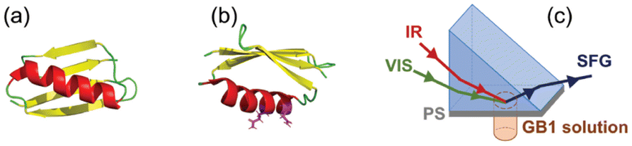

Fig. 1 (a) Crystal structure of WT GB1 (PDB ID: 3gb1). (b) Crystal structure of WT GB1 with Q32 and N35 plotted in magenta sticks. (c) Schematic of the SFG prism geometry used in this study to collect SFG spectra from the PS/protein solution interfaces.

The detected SFG intensity (I_SFG) can be expressed as:^12–30

where χ⁽²⁾_eff is the effective second-order susceptibility and χ⁽²⁾_NR is the non-resonant contribution. A_q, ω_q, and Γ_q are the SFG signal amplitude, the vibrational frequency (peak center), and the damping coefficient (peak width) of the vibrational mode q, respectively. These parameters can be obtained by fitting an SFG spectrum, and an SFG spectrum can be constructed if these parameters are available. The fitting parameters of the SFG spectra used for the protein spectral reconstruction in this study are listed in ESI Section S3.†

Atomistic MD simulation

The Gromacs⁶¹ (version 2019.6) simulation package was used to conduct atomistic MD simulations. The CHARMM 36 force field⁶² combined with a TIP3P water model was applied to describe the interactions in the system. The velocity Verlet algorithm was used for the dynamic equations with a time step of 1 fs. The long-range electrostatic interactions were calculated by the particle mesh Ewald (PME) summation with a cutoff of 1.2 nm. A spherical cutoff of 1.2 nm was imposed on Lennard–Jones interactions. The Parrinello-Rahman method was used to keep the NPT ensemble at 1 bar. The temperature was maintained at 298.15 K by the Berendsen thermostat. Periodic boundary conditions were applied to the system, along the X and Y directions only.

For WT GB1, we used a crystal structure (PDB code: 3gb1) from the Protein Data Bank (http://www.ncbi.nlm.nih.gov/). The MT GB1 protein structure was predicted by I-TASSER^63–65 based on the crystal structure of WT GB1. With amino acids lysine (Lys) protonated, glutamate (Glu) and aspartate (Asp) deprotonated, and uncapped N- and C-terminals, both WT and MT GB1 proteins have a net charge of −4e at pH of 7. Both proteins were relaxed in water at 298.15 K in the NVT ensemble before being assembled with the PS substrate surface.

An amorphous PS surface was constructed with 78 polystyrene chains. Each chain consists of 20 monomers. The PS surface was initially relaxed in a vacuum with a series of simulations of 30 ns for a total of 270 ns, which were carried out using a stepwise heating/annealing protocol starting at 298.15 K, reaching 700 K and then recovering to 298.15 K. Then the surface was exposed to water solution for further relaxation for 150 ns. The equilibrated PS surface is around 6.847 × 6.797 nm² in the X–Y plane with a thickness of 5.506 nm. After this, the hydrated PS surface was assembled with a protein, leaving an initial gap of at least 2.0 nm between the PS surface and the protein. The total dimension of the solvation box along the Z direction is 13.787 nm. Sodium counter ions were added to neutralize the system. The assembled initial configurations of WT GB1/PS and MT GB1/PS systems are shown in ESI Section S4.†

One-exciton Hamiltonian approach for SFG spectral calculation

In this study, a one-exciton Hamiltonian approach was adopted to calculate SFG spectra as a function of protein orientation. This methodology was reported previously⁵⁵ and also in our recent publications.^39,53 Since this method will be used to calculate the SFG spectra with isotope labeled units, which is a new feature, it will be briefly introduced here. A Hamiltonian matrix was constructed to obtain the SFG signal frequency and the strength of each amide I normal mode of a protein by using the couplings among the local modes of the amide units. Here, the diagonal terms of the Hamiltonian matrix, representing the local mode frequencies, were set to 1640 cm⁻¹ for non-isotope-labeled amide units and set to 1610 cm⁻¹ for isotope-labeled amide units. The off-diagonal terms of the Hamiltonian matrix, representing the coupling between each pair of amide units, were calculated according to the distance and the orientation of each amino acid. To calculate such couplings, this Hamiltonian approach requires a protein structure as the input. The normal modes and the vibrational frequency of each mode can be obtained by diagonalizing the constructed Hamiltonian matrix. The SFG signal strength can then be calculated for each amide I vibration normal mode. According to eqn (1), the SFG resonant susceptibility of each normal mode can be obtained by rationally assuming a peak width (10 cm⁻¹ in this study) and the overall SFG spectrum from the protein amide I mode can be acquired by using the sum of the SFG resonant susceptibility from all the amide units (omitting the χ⁽²⁾_NR term) for a specific protein orientation. The protein can be rotated and the SFG spectra can be calculated as a function of the protein tilt angle θ and twist angle ψ. The (tilt angle, twist angle) pair, also denoted as (θ, ψ), was used to define the orientation of a protein at the interface. The original orientation (0°, 0°) was defined as the protein orientation of the input protein structure, e.g., the crystal structure in the protein data bank or the orientation deduced from the computer simulation as described above. More details of the Hamiltonian spectra calculation method can be found in previous publications (46, 61). The calculated SFG response in the laboratory frame can be converted to the Jones frame to compare to the experimentally collected data (ESI Section S5†).

For spectra comparison, only the resonant spectra were compared, without the non-resonant contribution χ⁽²⁾_NR (See ESI Section S3†). A score system was developed to evaluate the similarity between the calculated SFG spectra and the experimental measurement, as illustrated in ESI Section S5.† The best matching score obtained from the comparison provides the most likely conformation (the input structure) and orientation (defined using (θ, ψ)) of the interfacial protein.

Results

SFG measurements

Fig. 1(a) displays the crystal structure of WT GB1 (PDB ID: 3gb1), showing that the GB1 crystal structure contains both α-helical and β-sheet structures. The two amino acids Q32 and N35 which will be mutated are both located in the helix, as shown in Fig. 1(b). SFG spectra were collected from protein molecules at the PS/protein solution interfaces using the experimental geometry presented in Fig. 1(c). Eight protein samples in total including two WT GB1 samples and six MT GB1 samples were prepared and studied in this research: non-labeled WT GB1 (WT NL), Leu-labeled WT GB1 (WT Leu), non-labeled MT GB1 (MT NL), Leu-labeled MT GB1 (MT Leu), Val-labeled MT GB1 (MT Val), Phe-labeled MT GB1 (MT Phe), Lys-labeled MT GB1 (MT Lys) and Ile-labeled GB1 (MT Ile). Fig. 2 and 3 display the collected SFG ssp and ppp spectra for all eight protein samples at the PS/protein solution interfaces. The spectral fitting results are also shown in the figures. The spectral fitting method and the fitting parameters are presented in the ESI (Section S3).† A positive peak at ∼1625 cm⁻¹ and a negative peak at ∼1655 cm⁻¹, assigned to the β-sheet structure^35,49 and α-helix structure^35,49 respectively, were detected in both the SFG ssp and ppp spectra of each of the eight samples. The opposite phases showed that the overall dipoles of the GB1 structural domains contributed to the 1625 cm⁻¹ and 1655 cm⁻¹ peaks point to opposite absolute orientations. The signal strengths of these two peaks could be acquired from the spectral fitting parameters. The small side peaks at ∼1690 cm⁻¹ observed in the ssp spectra of MT GB1 samples could be assigned to β-turns.^26,35 The other weak signals detected at ∼1740 cm⁻¹ in both SFG ssp and ppp spectra of all eight samples could be assigned to protein side chains and will not be included in the spectral comparison for the protein amide I signals.

Fig. 2 SFG ssp spectra collected from proteins (a) WT NL, (b) WT Leu, (c) MT NL, (d) MT Leu, (e) MT Val, (f) MT Phe, (g) MT Lys and (h) MT Ile adsorbed at the PS/protein solution interfaces. Black dots are experimental data points and red lines are fitted spectra.

Fig. 3 SFG ppp spectra collected from proteins (a) WT NL, (b) WT Leu, (c) MT NL, (d) MT Leu, (e) MT Val, (f) MT Phe, (g) MT Lys and (h) MT Ile absorbed at the PS/protein solution interfaces. Black dots are experimental data points and red lines are fitted spectra.

A dominant SFG peak observed in the ppp spectra of all the samples is centered at ∼1600 cm⁻¹, which could be generated from the C=C stretching mode of the phenyl groups on the PS side chains, as well as the amide I mode (mainly contributed by the ¹³C=O stretching) of the isotope labeled amide units of the protein. This peak was also detected in the ppp spectra collected from the PS/D₂O (without proteins) interface (ESI, Section S2†) and the PS/non-isotope-labeled protein (WT NL or MT NL) solution interfaces (Fig. 3(a) and (c)). The intensity of this peak was twice as intense as that of a normal protein amide I peak (e.g., a peak assigned to a β-sheet structure or an α-helix structure). Generally, the intensity of an isotope-labeled amide I peak of a protein should be very weak because of the low population of such amide units (which can be proved from the spectral calculation shown below). Therefore, here we believe that the intense peak observed at ∼1600 cm⁻¹ in the ppp spectra mainly comes from the phenyl groups of the PS side chains, instead of the isotope-labeled units of proteins. We thus decided that it is reasonable to exclude this peak when reconstructing the experimentally measured ppp spectra for later spectral comparisons with the calculated ppp spectra. For SFG, isotope labeling not only shifts the peak center of the amide I signal from the isotope labeled units, but it also changes the signal couplings between the isotope labeled units and other non-labeled units, leading to changes in the spectral features and intensities of the amide I signals from the non-labeled units of the protein. Thus, such changes in the spectra of the non-labeled protein units can also be used to quantify the isotope labeling effects.

Atomistic MD simulation results

Here, atomistic MD simulations were conducted to study the WT GB1 and MT GB1 samples without introducing isotope-labeling. We assume that isotope-labeling has negligible effects on the protein structure in solution and protein–PS interactions. Therefore, the non-labeled and isotope labeled WT GB1 (or MT GB1) samples have the same structure (same conformation and orientation) at the PS/protein solution interface. To ensure that we capture the equilibrated protein–polymer interaction, the MD run was performed for 1000 ns. Section S6 in the ESI† shows the distance between the protein (WT GB1 or MT GB1) and the PS surface as a function of time. According to this distance plot, the adsorption process happened quickly in both cases (∼20 ns for WT GB1 and ∼10 ns for MT GB1). For MT GB1 and WT GB1, the mean values and fluctuations of the radius of gyration (R_g) and the root mean square deviation (RMSD) are similar over the course of simulation (shown in ESI Sections S7 and S8 †), indicating that the mutation of Q32A and N35A would not cause substantial conformation changes of MT GB1 due to the GB1–PS interactions. The structures of WT GB1 and MT GB1 were similar and stable after GB1's landing on the PS surface. The secondary structure revolution maps (ESI Section S9†) show that WT GB1 and MT GB1 have similar conformations over the entire simulation time.

To quantify the orientation fluctuation of the α-helical portion of WT GB1 and MT GB1, we defined a tilt angle θ_a to evaluate the angle between the Z axis (the PS/protein solution interface normal) and the sum of amide I vectors from residue 21 to residue 36 (the α-helical portion, pointing from near the N- terminal to near the C-terminal) of protein GB1. The time-dependent θ_a plots of WT GB1 and MT GB1 (shown in ESI Section S10†) indicated that θ_a reached equilibrium after 600 ns for both proteins. However, the θ_a distributions of the last 400 ns of the simulations of WT GB1 and MT GB1 exhibited different mean values with similar standard deviations, indicating that the α-helical structures in WT GB1 and MT GB1 adopted different preferred orientations on the PS surface although they had similar conformations. It is interesting to observe that only mutating two amino acids of GB1 could change the protein orientation on PS substantially. This suggests that the mutation of Q32A and N35A alters the interactions between the GB1 protein and the PS surface, and the planar residues Q32 and N35 play an important role in such interactions. Similar phenomena were previously observed for WT GB1 and MT GB1 on graphene,⁵² which will be discussed in more detail later.

Spectral matching for WT GB1

SFG spectra can be calculated using the Hamiltonian method as we demonstrated previously.^39,53 To determine the interfacial protein conformation, for the Hamiltonian spectral analysis, protein configurations in the last 400 ns of the simulation were used. Due to the fluctuations and roughness of the soft surfaces of the PS film and protein GB1, the orientation of a landed protein can have small changes at a microsecond temporal scale. The atomistic MD simulation (≤1 μs) might not catch the slow tumbling (i.e. side rotation of a non-principle axis) of an adsorbed GB1 molecule on the PS surface.^58,66–69 In contrast, SFG experiments measure the averaged conformations of multiple proteins at the macro-scale. To overcome the defect of insufficient sampling in MD simulations, for the Hamiltonian SFG spectra calculation, we first rotated each MD simulated configuration of WT GB1 in the last 400 ns (1 ns per configuration) to (θ, ψ) from its initial orientation (0°, 0°) to compensate for the orientation fluctuations (θ ∈ [0°, 180°], ψ ∈ [0°, 360°], 5° as a step). It is worth noting that, although an orientation grid search was conducted, the final deduced orientation which best matches the experimentally measured spectra should be close to its initial state to match the atomistic MD simulation result. All 400 protein configurations and their rotated structures were used to calculate the ssp and ppp SFG spectra for WT NL and WT Leu (WT NL and WT Leu used the same protein structure but a different Hamiltonian matrix, as illustrated in the Method section below). Therefore, for each protein sample (WT NL or WT Leu), we calculated 400 × 180/5 × 360/5 = 1 036 800 ssp spectra and 1 036 800 ppp spectra. The calculated spectra were scored by comparing them to the experimentally reconstructed spectra for both spectral features and relative ssp/ppp spectral intensity. More details for SFG spectral calculation and for obtaining the matching scores from the comparison between calculated and reconstructed experimental spectra can be found in the Materials and Methods Section and Section S5 of the ESI† as well as our previous publication.³⁹ A heat map showing such matching scores as a function of protein orientation can be obtained for each of the 400 simulated configurations. The overall heat map for each simulated configuration can be obtained by combining the heat maps of the non-labeled and all isotope labeled samples of each configuration. The simulated configuration with the overall heat map with the maximum matching score among the 400 generated overall heat maps was chosen as the most likely conformation. The orientation with the highest matching score from the chosen heat map was selected as the most likely orientation. For WT GB1, considering the results for both WT NL and WT Leu, it was found that among all the possible candidates, the simulated WT GB1 structure at 781 ns with an orientation of (30°, 50°) or (150°, 230°) has the highest score (0.66). The heat map showing the matching scores of WT GB1 based on the simulated structure at 781 ns as a function of protein orientation is shown in Fig. 4(a). Clearly the heat map shows that the orientations (30°, 50°) and (150°, 230°) have the highest scores. In this study we performed homodyne SFG measurements to measure SFG signal intensity; thus the orientations of (θ, ψ) and (180° − θ, 180° + ψ) could not be differentiated. Here, (30°, 50°) and (150°, 230°) have the opposite absolute orientations.

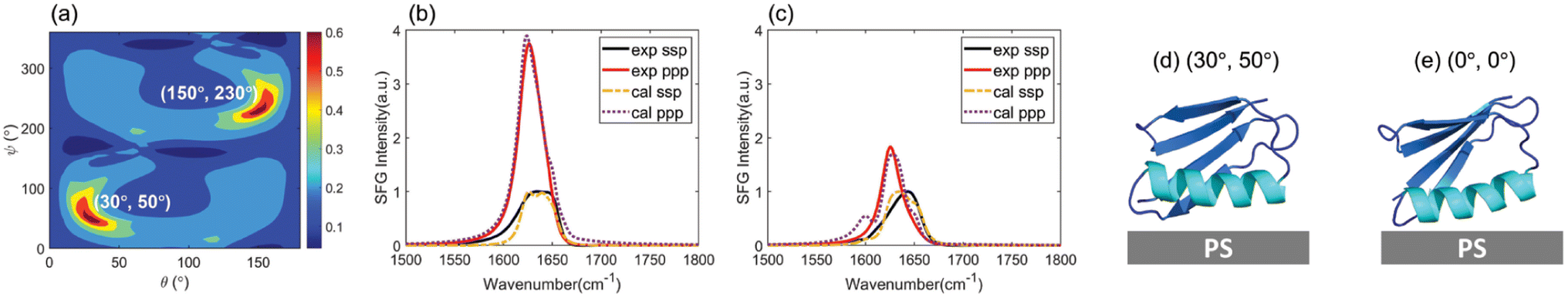Fig. 4 (a) Final score map of the spectral matching between the reconstructed experimentally collected WT GB1 SFG spectra (after deconvoluting the non-resonant contribution in ssp and ppp spectra and PS contribution in the ppp spectra) and the calculated WT GB1 SFG spectra as a function of protein orientation based on the simulated WT GB1 structure at 781 ns. The orientations at (30°, 50°) and (150°, 230°) in the map possess the highest matching scores (0.66). The spectral comparisons (b) between the reconstructed WT NL SFG spectra and the calculated WT NL spectra (based on the simulated structure at 781 ns) and (c) between the reconstructed WT Leu SFG spectra and the calculated WT Leu spectra (based on the simulated structure at 781 ns) at an orientation of (30°, 50°) (or (150°, 230°)) which have the highest matching scores. The orientation visualizations of (d) WT GB1 (with the 781 ns simulation structure) at (30°, 50°) and (e) WT GB1 (with the 781 ns simulation structure) at (0°, 0°). The (0°, 0°) orientation is the protein orientation obtained from the MD simulation result without further rotating the protein.

For WT GB1 with the orientation of the highest matching score, we plotted the calculated SFG ssp and ppp spectra from WT NL (Fig. 4(b)) and WT Leu (Fig. 4(c)) proteins. For comparison, re-constructed experimentally detected SFG spectra are also displayed in Fig. 4(b) and (c). From the spectral comparison results, one could find that the spectral features (peak center, peak intensity ratio of ppp/ssp, peak width, etc.) could be well-matched between the calculations and the experimental measurements, except for the isotope-labeled peak ∼1600 cm⁻¹ in WT Leu's case for the ppp spectrum. The calculated ppp spectrum of WT Leu shows the isotope labeled signal at ∼1600 cm⁻¹, which is missing in the reconstructed ppp spectrum. As we mentioned above, the mismatch could be due to the removal of the ∼1600 cm⁻¹ peak during the experimental spectral reconstruction since such a peak could come from the PS surface. Although the isotope-labeled peak was removed during the experimental spectral reconstruction due to its overlap with the PS signal, the match based on the main amide I peaks (from β-sheet/turn structure and α-helix structure) is still satisfactory.

Fig. 4(d) and (e) display the orientation visualizations of the deduced most likely (or best matched) orientation (30°, 50°) and the orientation obtained from the MD simulation without rotation (0°, 0° – the input structure for the Hamiltonian calculation) respectively. The best matched orientation (30°, 50°) showed that the α-helical structure lies down on the PS surface, while the β-sheet portion faces towards the solvent. This orientation is similar to an initial (0°, 0°) orientation obtained from the MD simulation at 781 ns without rotation, indicating that the orientation deduced from the SFG experimental data corroborates the MD simulation data. Furthermore, for the deduced best matched orientation, the θ_a value was deduced to be 90.2°. This value falls within the θ_a distribution of simulated WT GB1 for the last 400 ns of the MD simulations (see ESI Section S10†), further demonstrating that the deduced orientation from the experimental data well matches the simulation results. Meanwhile, the other best matched opposite absolute orientation (150°, 230°) (visualized in ESI Section S11†) with the α-helical structure far from the PS surface, was very different from its initial simulated orientation, which should be excluded because it failed to match the atomistic MD simulation results.

The close contact of the alpha-helical structure of WT GB1 with the PS surface is reasonable because of the strong interactions between the PS phenyl groups and the “planar” amino acids on the helix. More detailed discussion on the GB1–PS interactions will be presented below.

Spectral matching for MT GB1

We then used a similar approach to that discussed above for WT GB1 study to deduce the MT GB1 structure on PS. The last 400 MT GB1 configurations obtained from the MD simulations and their rotated structures were used to calculate the ssp and ppp SFG spectra for MT NL and isotope-labeled MT GB1 samples. An overall heat map showing the matching scores for each simulated configuration can be obtained by considering the matching qualities of the spectra generated from the non-labeled and all the isotope labeled samples including MT NL, MT Leu, MT Val, MT Phe, MT Lys and MT Ile. The heat map with the maximum matching score among all the heat maps of the 400 configurations (with rotations) was selected, as shown in Fig. 5(a).

Fig. 5 (a) Final score map of spectral matching between the reconstructed experimentally collected MT GB1 SFG spectra (after deconvoluting the non-resonant contribution in ssp and ppp spectra and PS contribution in the ppp spectra) and the calculated MT GB1 SFG spectra as a function of orientation based on the simulated MT GB1 structure at 972 ns. The orientations at (30°, 100°) and (150°, 280°) shown in the map possess the highest matching score (0.19). The spectral comparisons between the reconstructed experimental spectra and calculated spectra using the simulated MT structure at 972 ns with an orientation of (30°, 100°) (or (150°, 280°)) for (b) MT NL, (c) MT Leu, (d) MT Val, (e) MT Phe, (f) MT Lys and (g) MT Ile. The orientation visualizations of (h) MT GB1 with a simulated structure at 972 ns with the most likely orientation at (30°, 100°) and (i) MT GB1 with a simulated structure at 972 ns without rotation at (0°, 0°).

The best matched result for MT GB1 was found to be the simulated structure at 972 ns with an orientation of (30°, 100°) or (150°, 280°). The comparisons between the calculated spectra from different samples at this orientation with this conformation and the reconstructed experimental data are shown in Fig. 5(b)–(g). The best matched structure (30°, 100°) and the simulated structure (0°, 0°) are displayed in Fig. 5(h) and (i). The initial orientation of the simulated MT GB1 at 972 ns without rotation (Fig. 5(i)) showed that the α-helix was tilted up (θ_a = 144.2°) on the PS surface and the anti-parallel β-sheet near the N-terminal was close to the PS surface, which is similar to its initial orientation with θ_a = 148.2°, while the anti-parallel β-sheets lie down towards the surface slightly more. The other best matched MT GB1 simulated structure at 972 ns of (150°, 280°) has an absolute orientation opposite to its initial orientation obtained from simulation (visualized in ESI Section S11†) with a θ_a of 31.8° and the anti-parallel β-sheet near the N-terminal is far away from the surface. Because of such discrepancies between the simulated orientation and experimentally deduced orientation, we believe that the orientation of (150°, 280°) is unlikely to be the possible orientation and should be excluded.

From our above analysis, it is clear that WT GB1 and MT GB1 adopt different structures on the PS surface. The difference could be confirmed by directly looking at their SFG spectra. The SFG spectral differences between WT NL and WT Leu (Fig. 4) are not the same as the spectral differences between MT NL and MT Leu (Fig. 5). For example, the SFG ppp/ssp intensity ratio (∼1625 cm⁻¹) of WT NL (∼4) is twice the ratio of WT Leu (∼2), while this ratio is ∼4 for both MT NL and MT Leu. Such spectral differences inferred the structure variations (i.e. different conformations and/or orientations) of WT GB1 and MT GB1 at the PS/protein solution interface.

For structure variations, we first compare their deduced best matched conformations. The conformation difference between WT GB1 781 ns and MT GB1 972 ns is not obvious with RMSD = 2.0 Å (shown in ESI Section S12†), but it is larger than the conformational fluctuations of both WT GB1 and MT GB1 over the entire simulation time (RMSD mean of WT is 1.5 Å and RMSD mean of MT is 1.3 Å). We believe that the conformation difference between WT GB1 and MT GB1 is real. In terms of orientation differences, the α-helical component of WT GB1 is more or less lying down on the PS surface, which is substantially different from the standing-up pose of the α-helical structure of MT GB1.

Crystal structure for SFG spectral calculation

To confirm that MD simulated structures may provide a better structural input for SFG spectra calculation, the crystal structure of WT GB1 (PDB ID: 3gb1) was also used to calculate the SFG ssp and ppp spectra of WT GB1 and MT GB1 using the Hamiltonian method for reference and comparison. The final score heat maps obtained based on the crystal structures of WT GB1 and MT GB1, along with the spectral comparisons of the top-ranking orientations are shown in ESI Section S13† and Fig. 6, respectively. The best matched results (Fig. 6(a) and (b)) of WT GB1 determined using the crystal structure input showed lying-down orientations, while for MT GB1, the best matched protein orientations (Fig. 6(d) and (e)) are standing-up posts. Although using the crystal structure for spectral calculations could still differentiate the orientations between WT GB1 and MT GB1 on the PS surface, the score of the best matched orientations of WT GB1 (0.56) or MT GB1 (0.15) is lower than that obtained by using the rotated simulated structures of WT GB1 (0.66) or MT GB1 (0.19), respectively. This indicates that the analysis accuracy obtained by using the crystal structure is not as high as that obtained by using the simulated GB1 structures. Thus, we believe that the atomistic MD simulation could capture the protein structure deviation from the crystal structure when considering the protein–surface interaction, improving the accuracy of the SFG data analysis.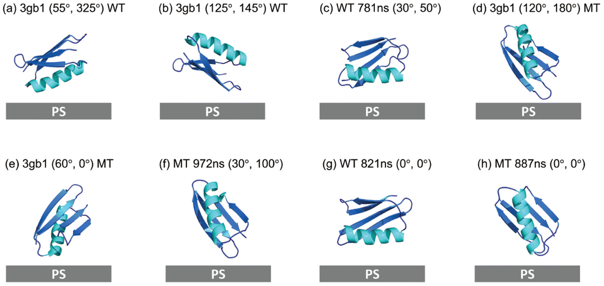

Fig. 6 Orientation comparisons of GB1 at the PS/protein solution interfaces: (a) and (b) the best matched orientations of WT GB1 based on the SFG data analysis using the GB1 crystal structure, (c) the best matched WT GB1 orientation after rotating all the simulated structures (based on the simulated structure at 781 ns) – replotted from Fig. 4(d). (d) and (e) The best matched orientations of MT GB1 based on the SFG data analysis using the GB1 crystal structure, (f) the best matched MT GB1 orientation after rotating all the simulated structures (based on the simulated structure at 972 ns) – replotted from Fig. 5(h). (g) The best matched WT GB1 orientation from the simulated structure without rotation (based on the simulated structure at 821 ns), and (h) the best matched MT GB1 orientation from the simulated structure without rotation (based on the simulated structure at 887 ns).

Discussion: comparison between interfacial WT GB1 and interfacial MT GB1

To understand the importance of rotating the protein to find the best match, the matching scores of all the simulated configurations (for the last 400 ns) at their initial orientation (0°, 0°) without rotation were compared for both WT GB1 and MT GB1. Detailed comparisons are shown in ESI Section S14–S17.† The top five best matches for the non-rotated simulated structures of WT GB1 are those obtained at 821 ns (Fig. 6(g), with a score of 0.37), 927 ns, 997 ns, 967 ns and 993 ns (shown in ESI Section S16†). For MT GB1, the top five such structures are those at 887 ns (shown in Fig. 6(h), with a score of 0.17), 817 ns, 927 ns, 820 ns and 765 ns (shown in ESI Section S17†). For both WT GB1 and MT GB1, although the visualized orientations deduced with and without rotation of the simulated structures are not very different, the best matched scores using non-rotated configurations are lower than those obtained by using rotated configurations. Rotating the simulated structures leads to the determination of protein structures with higher accuracy.

In our previous studies on GB1 on graphene, we found that planar amino acid residues play dominant roles in protein–graphene interactions through π–π interactions.⁵² Five out of the ten non-charged planar residues of WT GB1 (F30, Q32, Y33, N35, and N37) are in the α-helical chain (shown in Fig. 7(a)). They have strong interactions with the graphene surface to cause a complete denaturation of WT GB1 on graphene, as shown by both coarse grained MD simulation and the absence of a detected SFG signal.⁵² Here, PS has many phenyl groups, which can have strong π–π interactions with GB1 planar amino acids, but not as strong as those between graphene and WT GB1. Therefore, SFG signals of WT GB1 on PS could still be detected, showing that WT GB1 does not denature completely. On graphene, it is possible that WT GB1 needs to unfold for its side chains to come into good contact with the rigid planar graphene surface. However, in the case of PS, the PS surface roughness and molecular flexibility may be able to accommodate the protein–surface interaction better.

Fig. 7 Orientation visualizations of (a) the simulated WT GB1 structure at 781 ns of (30°, 50°) and (b) the simulated MT GB1 structure at 972 ns of (30°, 100°). Residues Q32 and N35 are shown in magenta sticks. Residues F30, Y33 and N37 are shown in red sticks.

Among the five planar residues in the helical structure, our SFG studies and MD simulations showed that Q32 and N35 are facing towards the PS surface for better interaction with the PS surface. After mutating the residues Q32 and N35 into alanine, the π–π interactions between the α-helical chain of MT GB1 and PS were greatly reduced. Therefore the α-helix does not lie down on the PS surface anymore. When the dominating π–π interaction between the protein and polymer is not dominating (caused by the mutation), other interactions can dominate and enable protein GB1 to adopt a varied orientation. For example, the hydrophilic amino acids (e.g. E27, K28 and K31) in the helix interact with water more favorably, leading to the tilt orientation of protein GB1 as determined. It is worth mentioning that as we demonstrated in our previous research on peptide or enzyme–MoS₂ interactions, π–π interaction does not play a dominating role, while other interactions such as hydrophobic/hydrophilic interaction can mediate the protein–surface interaction.^70,71 Our results agreed with this analysis and showed that the MT GB1 helix more or less stands up on the PS surface (Fig. 7(b)).

To consider the experimental errors and the possible structural fluctuations of proteins at interfaces, we plot all possible WT GB1 and MT GB1 structures which have matching scores of 90% or higher compared to the highest matching scores. Two movies in ESI Section S20 and S21 † show such structures of WT GB1 (with scores between 0.59 and 0.66) and MT GB1 (with scores between 0.17 and 0.19). Out of the 1 036 800 structures, seven WT GB1 and one hundred MT GB1 structures were found. All the WT GB1 structures are similar, with the α-helix lying down, while all the MT GB1 structures are similar, with the α-helix more or less standing up. MT GB1 represents more possible structures on the PS surface than WT GB1 (one hundred vs. seven), indicating that MT GB1 has greater structure flexibility and has less interaction with the PS surface.

Conclusion

A systematic strategy, combining SFG experimental measurements, isotope labeling, atomistic MD simulation, and Hamiltonian spectral calculation was developed to successfully deduce the conformations and orientations of WT GB1 and MT GB1 at the PS/protein solution interface in situ. Such conformations and orientations were determined by finding a protein structure which has the best matching quality between the experimentally measured SFG spectra and calculated SFG spectra using the Hamiltonian approach. The matching considers all the spectra from non-labeled and different isotope labeled samples. Isotope labeling greatly increases the number of independent measurements (parameters) for structural determination.

It was found that WT GB1 adopts an orientation with its α-helix lying down on the PS surface due to the strong π–π interactions between the PS phenyl groups and the planar residues in the helical structure of WT GB1. It was also found that MT GB1 has a different interfacial orientation, with the helix more or less standing up at the interface. These two orientations have different contact areas of the proteins with PS (ESI Section S17†). With Q32 and N35 amino acids replaced by alanine, the π–π interactions between the PS phenyl groups and the helix in MT GB1 were greatly reduced, enabling MT GB1 to stand up. This research shows that by mutating a very small number of some key amino acids in a protein, it is feasible to greatly vary the protein interfacial interactions to mediate interfacial protein structures.

Atomistic MD simulation is a powerful tool to capture protein–surface interactions to determine the protein interfacial structure. However, it is necessary to validate the simulation results with experimental data, which is challenging. This study provides a systematic approach using SFG to determine the protein interfacial structure with simulated results as inputs for SFG data analysis. The deduced protein structures with SFG measurements are more reliable than those using the protein crystal structure as the input structure.

Rapid progress has been made in protein expression and protein isotope labeling in recent years. With isotope selectively labeled proteins, many more independent measurements can be obtained using SFG, providing adequate parameters to determine interfacial protein structures at interfaces in situ. For the proteins with no known crystal structures, by using well-developed protein solution structure prediction software, we could predict protein solution structures from their sequence. With such predicted protein solution structures, we could use the methodology developed in this study to deduce their interfacial structures. Interfacial protein structures mediate interfacial functions, which play a significant role in many research areas and applications in chemistry, biology, medical sciences, and materials sciences and engineering. Determination of interfacial protein structures is significant and has broad impact.

Data availability

Data supporting the findings of this work are available within the paper and its ESI.† Additional data related to this paper may be requested from the author E-mail: zhanc@umich.edu on reasonable request.

Author contributions

W. G. and Z. C. designed the research. W. G., T. L., and R. C. performed SFG data collection and analysis. W. G. and T. W. carried out the molecular dynamics simulations. S. N. prepared the protein samples and characterized the samples with mass spectrometry. All the authors contributed to the manuscript preparation. The paper was read and approved by all the authors.

Conflicts of interest

The authors declare no conflicts.

Acknowledgements

Z. C. is thankful for the support from the National Science Foundation (CHE-1904380 to ZC) and the University of Michigan. T. W. is thankful for the support from the National Science Foundation (CBET-1943999). S. N. acknowledges the support provided by the Grant-in-Aid from JSPS for Fostering Joint International Research (A) (No. JP18KK0397).

References

1. J. Fu, W. Zhu, X. Liu, C. Liang, Y. Zheng, Z. Li, Y. Liang, D. Zheng, S. Zhu, Z. Cui and S. Wu, Nat. Commun., 2021, 12, 6907.
2. C. A. Del Grosso, C. Leng, K. Zhang, H.-C. Hung, S. Jiang, Z. Chen and J. J. Wilker, Chem. Sci., 2020, 11, 10367–10377.
3. H. Wang, D. E. Christiansen, S. Mehraeen and G. Cheng, Chem. Sci., 2020, 11, 4709–4721.
4. F. Sun, S. Suttapitugsakul and R. Wu, Chem. Sci., 2021, 12, 2146–2155.
5. K. Xue, K. T. Movellan, X. C. Zhang, E. E. Najbauer, M. C. Forster, S. Becker and L. B. Andreas, Chem. Sci., 2021, 12, 14332–14342.
6. A. A. Sanford, A. E. Rangel, T. A. Feagin, R. G. Lowery, H. S. Argueta-Gonzalez and J. M. Heemstra, Chem. Sci., 2021, 12, 11692–11702.
7. N. H. Joh, L. Thomas, T. R. Christian, A. Verlinsky, N. Jiao, N. Allotta, V. Jawa, S. Cao, L. O. Narhi and M. K. Joubert, J. Pharm. Sci., 2020, 109, 845–853.
8. J. Li, G. Chen, Y. Guo, H. Wang and H. Li, Chem. Sci., 2021, 12, 2876–2884.
9. S. Oh, M.-K. Lee and S.-W. Chi, Chem. Sci., 2021, 12, 5883–5891.
10. P. Prakash, K. P. Jethava, N. Korte, P. Izquierdo, E. Favuzzi, I. V. L. Rose, K. A. Guttenplan, P. Manchanda, S. Dutta, J.-C. Rochet, G. Fishell, S. A. Liddelow, D. Attwell and G. Chopra, Chem. Sci., 2021, 12, 10901–10918.
11. P.-S. Wang, H. Ma, S. Yan, X. Lu, H. Tang, X.-H. Xi, X.-H. Peng, Y. Huang, Y.-F. Bao, M.-F. Cao, H. Wang, J. Huang, G. Liu, X. Wang and B. Ren, Chem. Sci., 2022, 13, 13829–13835.
12. Y. R. Shen, Nature, 1989, 337, 519–525.
13. Z. Chen, Y. R. Shen and G. A. Somorjai, Annu. Rev. Phys. Chem., 2002, 53, 437–465.
14. X. Lu, C. Zhang, N. Ulrich, M. Xiao, Y.-H. Ma and Z. Chen, Anal. Chem., 2017, 89, 466–489.
15. J. Kim and P. S. Cremer, J. Am. Chem. Soc., 2000, 122, 12371–12372.
16. Q. Li, R. Hua, I. J. Cheah and K. C. Chou, J. Phys. Chem. B, 2008, 112, 694–697.
17. A. Perry, C. Neipert, B. Space and P. B. Moore, Chem. Rev., 2006, 106, 1234–1258.
18. F. M. Geiger, Annu. Rev. Phys. Chem., 2009, 60, 61–83.
19. T. Seki, K.-Y. Chiang, C.-C. Yu, X. Yu, M. Okuno, J. Hunger, Y. Nagata and M. Bonn, J. Phys. Chem. Lett., 2020, 11, 8459–8469.
20. Md. R. Khan, H. Singh, S. Sharma and K. L. Cimatu, J. Phys. Chem. Lett., 2020, 11, 9901–9906.
21. T. Weidner and D. G. Castner, Phys. Chem. Chem. Phys., 2013, 15, 12516.
22. H. Huang, C. Zhang, R. Crisci, T. Lu, H.-C. Hung, M. S. J. Sajib, P. Sarker, J. Ma, T. Wei, S. Jiang and Z. Chen, J. Am. Chem. Soc., 2021, 143, 16786–16795.
23. J.-J. Ho, A. Ghosh, T. O. Zhang and M. T. Zanni, J. Phys. Chem. A, 2018, 122, 1270–1282.
24. J.-J. Ho, D. R. Skoff, A. Ghosh and M. T. Zanni, J. Phys. Chem. B, 2015, 119, 10586–10596.
25. S. Ye, H. Li, W. Yang and Y. Luo, J. Am. Chem. Soc., 2014, 136, 1206–1209.
26. J. Tan, J. Zhang, Y. Luo and S. Ye, J. Am. Chem. Soc., 2019, 141, 1941–1948.
27. Z. Wang, H. Lin, X. Zhang, J. Li, X. Chen, S. Wang, W. Gong, H. Yan, Q. Zhao, W. Lv, X. Gong, Q. Xiao, F. Li, D. Ji, X. Zhang, H. Dong, L. Li and W. Hu, Sci. Adv., 2021, 7, eabf8555.
28. R. Pandey, K. Usui, R. A. Livingstone, S. A. Fischer, J. Pfaendtner, E. H. G. Backus, Y. Nagata, J. Fröhlich-Nowoisky, L. Schmüser, S. Mauri, J. F. Scheel, D. A. Knopf, U. Pöschl, M. Bonn and T. Weidner, Sci. Adv., 2016, 2, e1501630.
29. B. Wu, X. Wang, J. Yang, Z. Hua, K. Tian, R. Kou, J. Zhang, S. Ye, Y. Luo, V. S. J. Craig, G. Zhang and G. Liu, Sci. Adv., 2016, 2, e1600579.
30. H. Ye, A. Abu-Akeel, J. Huang, H. E. Katz and D. H. Gracias, J. Am. Chem. Soc., 2006, 128, 6528–6529.
31. S. Roy, P. A. Covert, W. R. FitzGerald and D. K. Hore, Chem. Rev., 2014, 114, 8388–8415.
32. S. Hosseinpour, S. J. Roeters, M. Bonn, W. Peukert, S. Woutersen and T. Weidner, Chem. Rev., 2020, 120, 3420–3465.
33. E. C. Y. Yan, Z. Wang and L. Fu, J. Phys. Chem. B, 2015, 119, 2769–2785.
34. X. Chen, M. L. Clarke, J. Wang and Z. Chen, Int. J. Mod. Phys. B, 2005, 19, 691–713.
35. B. Ding, J. Jasensky, Y. Li and Z. Chen, Acc. Chem. Res., 2016, 49, 1149–1157.
36. L. Fu, J. Liu and E. C. Y. Yan, J. Am. Chem. Soc., 2011, 133, 8094–8097.
37. W. Guo, T. Lu, Z. Gandhi and Z. Chen, J. Phys. Chem. Lett., 2021, 12, 10144–10155.
38. Z. Chen, Biointerphases, 2022, 17, 031202.
39. T. Lu, W. Guo, P. M. Datar, Y. Xin, E. N. G. Marsh and Z. Chen, Chem. Sci., 2022, 13, 975–984.
40. M. Bregnhøj, S. J. Roeters, A. S. Chatterley, F. Madzharova, R. Mertig, J. S. Pedersen and T. Weidner, J. Phys. Chem. B, 2022, 126, 3425–3430.
41. S. Alamdari, S. J. Roeters, T. W. Golbek, L. Schmüser, T. Weidner and J. Pfaendtner, Langmuir, 2020, 36, 11855–11865.
42. J. Zhang, J. Tan, R. Pei and S. Ye, Langmuir, 2020, 36, 1530–1537.
43. R. Verardi, N. J. Traaseth, L. R. Masterson, V. V. Vostrikov and G. Veglia, in Isotope labeling in Biomolecular NMR, ed. H. S. Atreya, Springer Netherlands, Dordrecht, 2012, vol. 992, pp. 35–62.
44. T. O. Zhang, M. Grechko, S. D. Moran and M. T. Zanni, in Protein Amyloid Aggregation, ed. D. Eliezer, Springer New York, New York, NY, 2016, vol. 1345, pp. 21–41.
45. S.-H. Shim, R. Gupta, Y. L. Ling, D. B. Strasfeld, D. P. Raleigh and M. T. Zanni, Proc. Natl. Acad. Sci. U. S. A., 2009, 106, 6614–6619.
46. A. M. Woys, Y.-S. Lin, A. S. Reddy, W. Xiong, J. J. de Pablo, J. L. Skinner and M. T. Zanni, J. Am. Chem. Soc., 2010, 132, 2832–2838.
47. B. Ding, J. E. Laaser, Y. Liu, P. Wang, M. T. Zanni and Z. Chen, J. Phys. Chem. B, 2013, 117, 14625–14634.
48. M. Kirsten Frank, F. Dyda, A. Dobrodumov and A. M. Gronenborn, Nat. Struct. Biol., 2002, 9, 877–885.
49. E. T. Harrison, T. Weidner, D. G. Castner and G. Interlandi, Biointerphases, 2017, 12, 02D401.
50. R. Berkovich, J. Mondal, I. Paster and B. J. Berne, J. Phys. Chem. B, 2017, 121, 5162–5173.
51. S. Wei, L. S. Ahlstrom and C. L. Brooks, Small, 2017, 13, 1603748.
52. S. Wei, X. Zou, J. Tian, H. Huang, W. Guo and Z. Chen, J. Am. Chem. Soc., 2019, 141, 20335–20343.
53. W. Guo, X. Zou, H. Jiang, K. J. Koebke, M. Hoarau, R. Crisci, T. Lu, T. Wei, E. N. G. Marsh and Z. Chen, J. Phys. Chem. B, 2021, 125, 7706–7716.
54. S. J. Roeters, C. N. van Dijk, A. Torres-Knoop, E. H. G. Backus, R. K. Campen, M. Bonn and S. Woutersen, J. Phys. Chem. A, 2013, 117, 6311–6322.
55. P. Hamm and M. Zanni, Concepts and Methods of 2D Infrared Spectroscopy.Cambridge University Press, New York, NY, 2011.
56. T. Wei, H. Ma and A. Nakano, J. Phys. Chem. Lett., 2016, 7, 929–936.
57. T. Zhang, T. Wei, Y. Han, H. Ma, M. Samieegohar, P.-W. Chen, I. Lian and Y.-H. Lo, ACS Cent. Sci., 2016, 2, 834–842.
58. P. Sarker, M. S. J. Sajib, X. Tao and T. Wei, J. Phys. Chem. B, 2022, 126, 601–608.
59. S. V. Le Clair, K. Nguyen and Z. Chen, J. Adhes., 2009, 85, 484–511.
60. K. T. Nguyen, S. V. Le Clair, S. Ye and Z. Chen, J. Phys. Chem. B, 2009, 113, 12169–12180.
61. M. J. Abraham, T. Murtola, R. Schulz, S. Páll, J. C. Smith, B. Hess and E. Lindahl, SoftwareX, 2015, 1–2, 19–25.
62. J. Huang, S. Rauscher, G. Nawrocki, T. Ran, M. Feig, B. L. de Groot, H. Grubmüller and A. D. MacKerell, Nat. Methods, 2017, 14, 71–73.
63. W. Zheng, C. Zhang, Y. Li, R. Pearce, E. W. Bell and Y. Zhang, Cells Rep. Methods, 2021, 1, 100014.
64. J. Yang, R. Yan, A. Roy, D. Xu, J. Poisson and Y. Zhang, Nat. Methods, 2015, 12, 7–8.
65. J. Yang and Y. Zhang, Nucleic Acids Res., 2015, 43, W174–W181.
66. T. Wei, M. A. Carignano and I. Szleifer, Langmuir, 2011, 27, 12074–12081.
67. T. Wei, M. A. Carignano and I. Szleifer, J. Phys. Chem. B, 2012, 116, 10189–10194.
68. C. M. Nakano, H. Ma and T. Wei, Appl. Phys. Lett., 2015, 106, 153701.
69. M. S. Jahan Sajib, Y. Wei, A. Mishra, L. Zhang, K.-I. Nomura, R. K. Kalia, P. Vashishta, A. Nakano, S. Murad and T. Wei, Langmuir, 2020, 36, 7658–7668.
70. M. Xiao, S. Wei, Y. Li, J. Jasensky, J. Chen, C. L. Brooks and Z. Chen, Chem. Sci., 2018, 9, 1769–1773.
71. M. Xiao, S. Wei, J. Chen, J. Tian, C. L. Brooks III, E. N. G. Marsh and Z. Chen, J. Am. Chem. Soc., 2019, 141, 9980–9988.

---

Footnote

† Electronic supplementary information (ESI) available. See DOI: https://doi.org/10.1039/d2sc06958j

---