Evaluation of the lead removal capacity by the adsorption process of Corbula trigona shell powder: modeling and optimization through reponse surface methodology

Abstract

This study is based on the evaluation of the adsorption process using Corbula trigona shell powder to remove lead from aqueous solution in a batch mode. Different analytical techniques, including X-ray diffraction, Fourier transform infrared spectroscopy, and EDS-coupled scanning electron microscopy, were used to characterize the shell powder before and after lead treatment. Regarding the pollutant removal, a Plackett–Burman design (PBD) was first used to determine the influencing factors from the following experimental domain: solution pH (3–9), adsorbent mass (0.1–0.5 g), contact time (40 –240 min), initial pollutant concentration (10 –60 mg L⁻¹), and adsorbent size (100 –200 μm). The respective contributions of the various factors listed above are 31.7%, 30.51%, 25.17%, 12.44%, and 0.18%. As a result, solution pH, adsorbent mass, contact time, and initial pollutant concentration were selected to optimize the lead removal process using the composite central plan. The optimal lead removal conditions were 99.028% by setting the solution pH to 4.5, initial lead concentration to 47 mg L⁻¹, contact time to 125 min, and adsorbent mass to 0.2 g. In addition, it was found that the composite central plan could be a reliable statistical tool to model and determine the optimal conditions.

---

1. Introduction

The fall in the cost of industrial raw materials in the Ivory Coast in 1980 led the Ivorian government to develop other sectors of activity, particularly the mining sector, to maintain its economy. Since this period, the Ivorian mining code has been revised to encourage mining companies to set up operations throughout the country.¹ However, in addition to this industrial activity, several gold panning sites have emerged in several localities of the country. However, this activity negatively impacts the soil, air, and water resources by disrupting the hydrographic network.^2–4 It also generated large quantities of wastewater that were directly discharged into the environment without any prior treatment.⁵ These mining effluents contribute a great deal to the pollution of water resources, as they contain trace metal elements, particularly lead, the concentration of which exceeds the standards set by the World Health Organization (WHO) at the rate of 255.5 μg L⁻¹.⁵ This environmental lead contamination can have harmful effects on human health. It can damage the liver and the brain as a result of its accumulation in either living tissues throughout the food chain or directly through ingestion.^6–8 In addition, lead exposure has been shown to be responsible for 853 000 deaths worldwide in 2013 due to its long-term health effects, especially in low- and middle-income countries.^9,10 Therefore, treatment and control of lead concentrations in wastewater from gold mines should be addressed. The main challenge is to set up a very effective method for lead removal below the standards set by the WHO (10 μg L⁻¹). It is in this configuration that several conventional methods have been set up for the treatment of wastewater containing trace metals. These methods include ion exchange, chemical precipitation, electrochemical treatment, electrocoagulation, evaporation, and adsorption.^11–13 Some of these methods are costly and often ineffective when the concentration of metals varies from 10 to 100 mg L⁻¹ and generate toxic sludge.¹⁴ Thus, the adsorption of metals on low-cost materials is an attractive alternative for the treatment of mining effluents loaded with trace metal elements.^12,15 However, the adsorption of pollutants on biomaterials or mollusc shells has been recognized as an effective method due to their composition.^16–18 With this in mind, this study focused on Corbula trigona shell wastes for the treatment of mining wastewater by the adsorption method. Corbula trigona shells are natural and constitute an abundant waste at the edge of the Ivorian lagoons, especially the Aby lagoon, which can be valorized. This available waste, in large quantities with an estimated mass of 1 147 000 tons, contributes to environmental pollution.¹⁹ However, to our knowledge, no study has been conducted on the absorption of lead on Corbula trigona shells. Moreover, studies on wastewater treatment using the classical method of varying one variable while fixing the others are long and do not allow observing the interactions between the different variables involved. To overcome this limitation, this study turned to the use of response surface methodology (RMS). The use of the response surface methodology in the adsorption process can improve the lead adsorption efficiency and reduce the number of experiments and the time of performing the different tests.²⁰ Thus, the overall objective of this study is to evaluate the adsorption capacity of lead by Corbula trigona shell powder. Thus, an experimental design methodology was used to investigate the influence of the main experimental parameters (lead concentration, solution pH, adsorbent size, adsorbent mass, and contact time). The specific objectives of this study are the following: (i) screen and quantify the effect of selected factors in the experimental domain using the Plackett–Burman design, (ii) optimize the mathematical model developed from a central composite design (CCD) to find the best combination of factors that leads to the best conditions for lead removal in solution.

2. Material and methods

2.1. Treatment and characterization of adsorbents

In this study, Corbula trigona shells were used as adsorbent material for the adsorption of lead in an aqueous solution. Those shells were collected from the beaches of the Aby lagoon located in the south-eastern region of the Ivory Coast. The shells were first washed several times with distilled water to remove impurities, and then they were dried in an incubator for 24 h at 105 °C. After drying, they were crushed in a porcelain mortar with a pestle and sieved to obtain two fractions of sizes less than or equal to 100 and 200 μm. The obtained grindings were preserved in jars. To better understand the mechanism of lead adsorption, the shell powder was subjected to a physicochemical characterization. The surface morphology and elemental composition of the shells before and after lead removal were determined by scanning electron microscopy (SEM) combined with Hitashi FEGS 4800 X-ray Dispersive Energy (EDX) microanalysis under an accelerating voltage of 15 kV. ALPHA Brucker Fourier Transform Infrared Spectroscopy (FT-IR) was used to analyze the chemical bonds and functional groups involved in lead adsorption in the range of 500–4000 cm⁻¹. Finally, an X-ray diffractometer (XRD, Rigaku Miniflex II) was used to analyze the different mineralogical phases of the materials.

2.2. Preparation of the lead solution

1.315 g of 98% purity lead chloride (PbCl₂) was dissolved in 1 L of ultrapure water to prepare a stock solution of 1 g L⁻¹ lead. This solution was diluted to prepare solutions of concentrations 10–60 mg L⁻¹. The initial pH of these solutions was adjusted from 3–9 by adding sodium hydroxide (NaOH, 0.1 M) or hydrochloric acid (HCl, 0.1 M) of 99% purity using a pH meter (Hanna pH 211).

2.3. Optimization of lead removal

To optimize the lead removal process, the experiments were performed in two phases. The first phase involved factor screening by the Plackett–Burman design method using the Hadamard matrix. The factors and levels (low (−1) and high (+1)) such as pollutant concentration (10–60 mg L⁻¹), solution pH (3–9), adsorbent size (100–200 μm), adsorbent mass (0.1–0.5 g), and contact time (40–240 min) are denoted as U₁, U₂, U₃, U₄, and U₅ respectively. All factors and their levels were selected based on preliminary and previous studies. 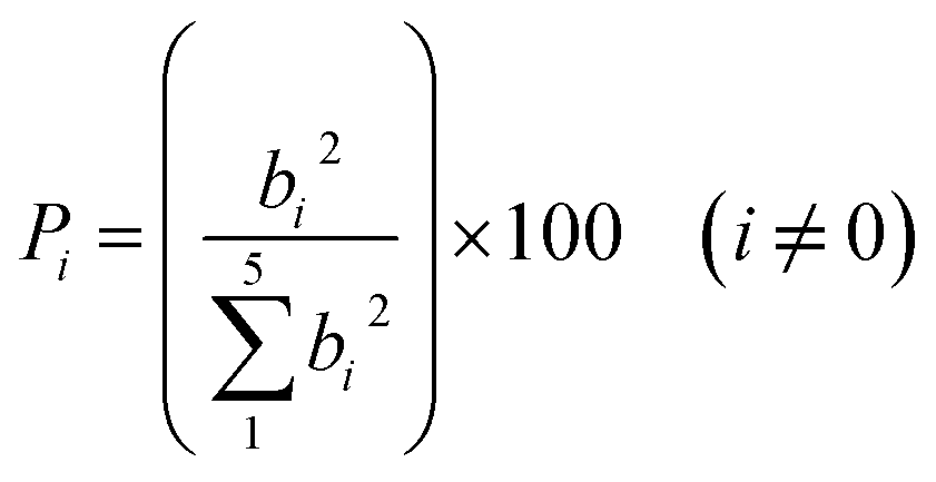With this design, the relationship linking the response to the different factors is given by (eqn (1)).²⁰where y, b_o, b_i and X_i, represent the experimental response (residual concentration), mean value of the responses from the 8 trials, main effect of each factor on the response, and coded variable of the factors (−1 or +1), respectively. Factors with coefficient values, i.e., bi with twice the standard deviation, are considered to influence the lead removal process.²¹ When the coefficient and its standard deviation are of the same order of magnitude, the influence of the factor is possible, in which case the experimenter must use his or her knowledge and the issues of the study to make a decision.²⁰ The contribution of factors (P_i) (eqn (2)), according to the Pareto chart, also evaluates the importance of the main factors on the response.

P_i is the contribution of factor i to the response, and bi is the statistical coefficient corresponding to factor i.

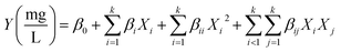
The second step was to use the concentration of the pollutant, pH of the solution, mass of the adsorbent, and contact time to model the responses by the response surface method (RMS) using a five-level composite central plane (CCD). This technique typically develops second-degree mathematical functions represented by (eqn (3)).

where Y is the response, β₀ is the constant factor, X² are variables, β_i is the linear, β_ii is the quadratic, and β_ij is the second-order interaction factor.

The composite central design was used to develop regression models and model the response, which is the residual lead concentration. The experimental ranges and (coded) levels of the independent variables that were determined by the experiments are shown in Table 1. A total of 30 experiments were performed in this work, including 16 experiments at the factorial points, 8 experiments at the axial point, and 6 replications at the central points. Data processing was performed using the NEMROD-W software (Version 9901 French, LPRAI-Marseille Inc., France). All experiments were performed in batches using 25 mL flasks into which we introduced 20 mL of the solution. Residual lead concentrations in the solutions after treatment were determined by an inductively coupled plasma optical emission spectrometer, Optima 8000, PerkinElmer (ICP-OES), after filtration on Whatman paper of 0.45 μm porosity.

Table 1 Experimental area of the composite central plan

Coded variables (Xi)	Factors	Experimental domain
		−2	−1	0	+1	+2
X1	Concentration (mg L^−1)	10	23	35	47	60
X2	pH	3	4.5	6	7.5	9
X3	Mass of the adsorbent (g)	0.1	0.2	0.3	0.4	0.5
X4	Contact time (min)	40	90	140	190	240

---

The percentage of lead removal was determined according to (eqn (4)).

C₀ (mg L⁻¹) and C_r (mg L⁻¹) are the initial and residual concentrations of lead.

3. Results and discussions

3.1. Characterization of Corbula trigona shells

The X-ray diffraction (XRD) study of Corbula trigona shells before and after lead adsorption is presented in (Fig. 1).

Fig. 1 X-ray diffraction patterns of Corbula trigona shell before (red) and after (black) lead adsorption.

Analysis of (Fig. 1) shows that the X-ray diffraction pattern of the shell before lead adsorption consists predominantly of calcite at 2θ = 29.4°. Calcite and aragonite peaks are also observed at 2θ = 20.92°; 23.76°; 26.68°; 28.32°; 36.6°; 37.52°; 39.52°; 42.92°; 47.52°; 48, 56°; 62.28°; 68.4°. Those results are in agreement with the reported work.²² After the adsorption of the pollutant, the major peak underwent a decrease with the appearance of cerussite on the surface. The same contact was made earlier²³ after the removal of lead, cadmium, and zinc by mollusc shells composed of aragonite and calcite. The reduction in the intensity of the calcite peak after lead adsorption could be due to an ion exchange between lead and Ca²⁺.

3.2. Characterization of the FT-IR spectrum

To determine the functional groups responsible for lead adsorption, IR analyses of Corbula trigona layers were performed (Fig. 2). The blue spectrum obtained before the removal of the pollutant shows two major peaks and vibrations. The two peaks around 1483.828 cm⁻¹ and 863.355 cm⁻¹ represent CO₃²⁻ carbonate groups.²⁴ The corresponding peak at 1483.828 cm⁻¹ represents the characteristic adsorption peak of calcite, while that of aragonite was observed at 863.355 cm⁻¹. Those results show that the shells of Corbula trigona contain mainly calcite and aragonite.^25–27 As for the vibrational bands, the one between 2510.466 cm⁻¹ and 1945.101 cm⁻¹ represents valence vibrations of the (O–H) groups of the carboxylic acid. The stretching vibration band from 3994.295 to 2581.902 cm⁻¹ is attributed to the water molecule in those shells or an organic compound that contains hydroxide groups (OH⁻). The orange spectrum obtained after lead removal shows changes in the vibrational peaks and the appearance of two new peaks, 714.279 cm⁻¹ to 1083.725 cm⁻¹. The peaks corresponding to carbonates 1483.828 cm⁻¹ to 863.355 cm⁻¹ increase to 1479.66 cm⁻¹ and 860.26 cm⁻¹, respectively. The appearance of the new peaks would be due to the interaction between lead and shells leading to the formation of PbCO₃, as reported in the literature.²⁸ The shift in peaks and the formation of PbCO₃ show that lead was precipitated together with carbonate carbonates.^29,30 The new peak 1081.725 cm⁻¹ can be related to the complexation of the carboxyl group with lead ions. We can say that the carbonate, hydroxyl, and carbonyl groups are implicated in the lead removal process from aqueous solutions. This shows that this removal occurs either by the exchange mechanism in which lead ions (Pb²⁺) bind to the adsorption sites replacing calcium ions (Ca²⁺) by precipitation, complexation, or adsorption, as shown by other authors.^26,31

Fig. 2 Fourier transform infrared (FTIR) spectra of Corbula trigona powder before (blue) and after (orange) lead adsorption.

3.3. Analysis by scanning electron microscopy (SEM) coupled with energy dispersive spectrometry (SEM/EDS)

The surface structure and morphology of Corbula trigona shells before and after adsorption were revealed by SEM analysis. It is clear from Fig. 3 that the biomaterials exhibited an irregular structure with an amount of rough structure, which could be advantageous for lead adsorption. The images show small particles attached to the surface. Those particles could be calcium salts (Ca²⁺), as reported by other authors.³² Fig. 4 shows that the surface of the materials became rougher with more porous areas after lead adsorption, and this fact could be related to the detachment of calcium (Ca²⁺) ions on the surface during the adsorption mechanism. Those ions could be replaced by lead molecules during the pollutant removal process. The EDS spectra (Fig. 3) before lead removal showed three major elements, calcium, oxygen, and carbon. After lead removal (Fig. 4), the peaks of the three elements decreased with the disappearance of silicon and the presence of lead. As for the content of the majority constituents, such as carbon, oxygen, and calcium, it was 25.49%, 64.80%, 22.24%, respectively. This result confirms the X-ray diffraction (XRD) analysis, which showed that the material contains calcium carbonate. After the adsorption of lead (Fig. 4), the mentioned results showed that the carbon content decreased by 3.79%, while that of oxygen and calcium increased by 0.72% and 2.86%, respectively. Finally, the observed functional groups could promote lead adsorption, as reported in the literature.^33,34

Fig. 3 Scanning electron microscopy (SEM) and X-ray (EDS) spectra of Corbula trigona shell powder before lead adsorption.

Fig. 4 Scanning electron microscopy (SEM) and X-ray (EDS) spectra of Corbula trigona shell powder after lead adsorption.

Fig. 5 shows the EDS mapping of the carbon, oxygen, and calcium distribution of the Corbula trigona shell composition, with the distribution of lead. The appearance of lead on the mapping shows that there is a binding of the lead molecule on the surface of the adsorbents.

Fig. 5 EDS mapping of shellfish after lead adsorption.

4. Study of lead adsorption

4.1. Plackett and Burman design (PPB)

The Plackett–Burman design was used to determine the influencing factors and their main effects on lead adsorption by Corbula trigona shells. After the tests were conducted, the experimental design and responses were recorded in Table 2.

Table 2 Experimental design and results on lead removal

No. test	Experimental design					Residual lead concentrations Y (mg L^−1)
	U1 (mg L^−1)	U2	U3 (μm)	U4 (g)	U5 (min)
1	60	9	200	0.1	240	0.263
3	10	9	200	0.5	40	0.112
2	10	3	200	0.5	240	0.136
4	60	3	100	0.5	240	0.281
5	10	9	100	0.1	240	0.144
6	60	3	200	0.1	40	0.659
7	60	9	100	0.5	240	0.261
8	10	3	100	0.1	40	0.548

---

Table 2 presents the results of 8 tests. Analysis of the results shows variability in residual lead concentrations with variation in factor levels. The residual concentrations range from 0.112 mg L⁻¹ to 0.659 mg L⁻¹ with a standard deviation of 0.1995. This variability in response means that one factor has at least an influence on lead adsorption by Corbula trigona shellfish and that the choice of experimental area is appropriate. The lowest residual concentration (0.112 mg L⁻¹) was obtained using 10 mg L⁻¹ of the pollutant at pH = 9, particle size of 200 μm, adsorbent mass of 0.5 g, and contact time of 40 min. The highest residual concentration, 0.659 mg L⁻¹, was obtained with a concentration of 60 mg L⁻¹ of lead, pH = 3, particle size of 200 μm, mass of 0.5 g, and time of 40 min. The estimates and statistics of the different coefficients related to the model factors are reported in Table 3.

Table 3 Coefficient estimates and statistics

Name	Coefficients	Standard deviation
bo	0.300	0.001
b1	0.066	0.001
b2	−0.105	0.001
b3	−0.002	0.001
b4	−0.103	0.001
b5	−0.094	0.001

---

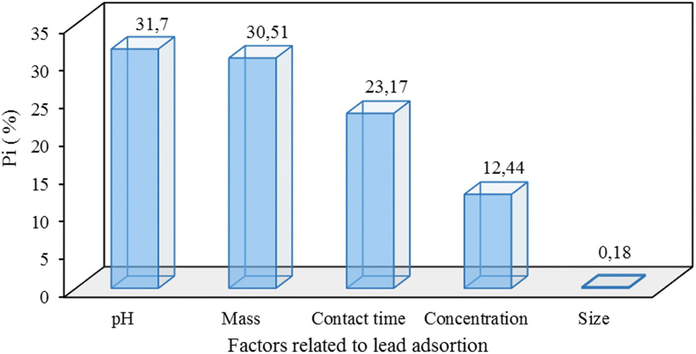
The significance test of each coefficient in the model was performed by assuming that a coefficient is significant if its absolute value is greater than two times the standard deviation.³⁵ Based on this, the mean coefficient b_o of the 8 trials and the main effects b₁ (0.066), b₂ (−0.105), b₄ (−0.103), and b₅ (−0.094) corresponding to initial pollutant concentration, solution pH, adsorbent mass, and contact time, respectively, are significantly different from zero. Size had no significant effect on lead removal. The Pareto chart was used to confirm the effect of each parameter on lead removal (Fig. 6).

Fig. 6 Pareto chart of the effects of different factors on the residual lead concentration.

This diagram shows that the pH of the solution, mass of the adsorbent, contact time, and concentration of the pollutant are the factors that influence most of the adsorption of lead by the shellfish. They have a contribution of 31.70%, 30.51%, 25.17%, and 12.44%, respectively, with a cumulative percentage of 99.82%. The size of the shells (X₃) contributes at a rate of 0.18% and does not influence the response in the studied experimental area. The adsorption of metal ions on these biomaterials is highly dependent on the pH of the solution, as the pH affects the degree of ionization and surface charge of the adsorbent.^17,36 This phenomenon could be related to a strong electrostatic attraction between the positively charged metal ions and the negatively charged sites of the Corbula trigona shell. As for the mass of the adsorbent, it also plays an important role in lead adsorption as it directly affects the process and must be carefully adjusted. It is evident that by increasing the mass of the adsorbent, the residual concentration decreases, which can be attributed to the availability of adsorption sites to capture the metal ions.³⁷ Contact time is the third factor affecting lead adsorption. Increasing the contact time contributes to a decrease in the residual concentration of lead in the solution. These results corroborate those reported in the literature on metal removal from oyster shells.^38–40 According to these results, metal adsorption from oyster shells is strongly dependent on three parameters: solution pH, adsorbent mass, and contact time. However, the process of metal removal from oyster shells is dependent on the initial concentration of the pollutant to be removed. At too high concentrations, removal appears to be inefficient. The sign of the coefficient corresponding to the initial concentration (b₁ = 0.066) is positive, showing that increasing the initial concentration negatively affects the lead adsorption.⁴⁰ Thus, four parameters were selected, solution pH, adsorbent mass, contact time, and pollutant concentration, to optimize pollutant removal.

4.2. Optimization of the lead removal process

The initial pollutant concentration (U₁), solution pH (U₂), adsorbent mass (U₃), and contact time (U₄) were considered as the independent factors or variables of the process. The individual and interactive effects of the factors on lead adsorption optimization were studied using the composite central design. A total of 30 trials were conducted according to the experimental design with the different responses in Table 4.

Table 4 Experimental design and results

No. test	Concentration initial (mg L^−1)	pH	Mass of adsorbent (g)	Contact time (min)	Experimental responses (mg L^−1)	Responses predicted (mg L^−1)
1	23	4.5	0.2	90	0.36	0.28
2	47	4.5	0.2	90	0.33	0.35
3	23	7.5	0.2	90	0.12	0.18
4	47	7.5	0.2	90	0.30	0.29
5	23	4.5	0.4	90	0.10	0.16
6	47	4.5	0.4	90	0.21	0.19
7	23	7.5	0.4	90	0.12	0.08
8	47	7.5	0.4	90	0.20	0.17
9	23	4.5	0.2	190	0.09	0.13
10	47	4.5	0.2	190	0.24	0.27
11	23	7.5	0.2	190	0.07	0.07
12	47	7.5	0.2	190	0.32	0.27
13	23	4.5	0.4	190	0.08	0.08
14	47	4.5	0.4	190	0.25	0.20
15	23	7.5	0.4	190	0.07	0.06
16	47	7.5	0.4	190	0.16	0.23
17	10	6	0.3	140	0.08	0.03
18	60	6	0.3	140	0.11	0.14
19	35	3	0.3	140	0.36	0.34
20	35	9	0.3	140	0.31	0.31
21	35	6	0.1	140	0.24	0.21
22	35	6	0.5	140	0.11	0.12
23	35	6	0.3	40	0.10	0.12
24	35	6	0.3	240	0.11	0.07
25	35	6	0.3	140	0.15	0.16
26	35	6	0.3	140	0.15	0.16
27	35	6	0.3	140	0.16	0.16
28	35	6	0.3	140	0.15	0.16
29	35	6	0.3	140	0.15	0.16
30	35	6	0.3	140	0.15	0.16

---

The values of the different regression coefficients as well as the significance levels are recorded in Table 5. It is noticeable that the linear coefficients b₁, b₂, b₃, and b₄, the quadratic effects b₁₁, b₂₂, b₄₄, and the interactions b₁₂, b₁₄, b₂₄, b₃₄ are significant at the 95% confidence level. Therefore, the statistically significant values of the parameters are as follows: the linear effect of all the factors or variables studied, the quadratic effect of initial concentration/initial concentration; solution pH/solution pH and contact time/contact time and interactions, initial concentration-solution pH; initial concentration-contact time; solution pH-contact time, and adsorbent mass-contact time.

Table 5 Estimates and statistics of lead adsorption coefficients

Name	Coefficients	Standard Deviation	Pr. > F
bo	0.161	0.001	< 0.01 ***
b1	0.066	0.001	< 0.01 ***
b2	−0.105	0.001	< 0.01 ***
b3	−0.043	0.001	< 0.01 ***
b4	−0.025	0.001	< 0.01 ***
b11	−0.075	0.003	< 0.01 ***
b22	0.165	0.003	< 0.01 ***
b33	0.005	0.003	12.1
b44	−0.065	0.003	< 0.01 ***
b12	0.013	0.003	< 0.01 ***
b13	−0.006	0.001	0.168 **
b14	0.020	0.001	< 0.01 ***
b23	0.008	0.001	0.0732 **
b24	0.014	0.001	< 0.01 ***
b34	0.020	0.001	< 0.01 ***

---

A quadratic polynomial model was selected to develop the thematic relationship between the independent process variables and the responses. The mathematical (eqn (5)) describing the variation of the residual concentration can be written as a function of coded variables.

Y (mg L⁻¹) = 0.161 + 0.057X₁ − 0.019X₂ − 0.043X₃ − 0.025X₄ − 0.075X₁² + 0.165X₂² − 0.065X₄² + 0.013X₁X₂ + 0.02 X₁X₄ + 0.014X₂X₄ + 0.020X₃X₄ (5)

4.2.1. Model validation. The statistical significance of the composite central design model was investigated by ANOVA, and the results are presented in Table 6. The results showed that the obtained model could be successfully used in the studied experimental area. Indeed, according to the statistical treatment, the values of the coefficient of determination were (R² = 0.854 and R² aj = 0.718). The regression model could well explain the lead removal process because the coefficient of determination must be greater than or equal to 0.80 for a good fit of a model.^41,42 The analysis of variance (ANOVA) of the parameters of the quadratic predicted response surface model for lead removal parameters shows that the model is significant with F-value of 892.755 and a low probability value ((Pr. > F) ≪ 0.01). Indeed, when using a confidence level of 0.05, a model is considered significant if the probability value p is less than 0.05. The representation of the observed values and the predicted values also give important information about the adequacy of the model. Fig. 7 shows that the predicted values and the experimental values are distributed around the regression line (R² = 0.854) greater than 0.8, which reflects good conformity between those different values.⁴³ Therefore, the model is valid.

Table 6 Analysis of variance of the second degree model

Source of variation	Sum of squares	Degrees of freedom	Mean square	F-value	Pr. > F
Regression	0.0208 310	14	0.0148 792	892.7556	< 0.01 ***
Residuals	0.0355 070	15	0.00236 713
Validity	0.0354 237	10	0.00354 237	211.5421	< 0.01 ***
Error	0.0000833 333	5	0.000166 667
Total	0.243 817	29

---

Fig. 7 Residual graphs for percent lead removal.

4.2.2. Graphical analysis of the results. The influence of pH and the initial concentration of the pollutant on the removal are represented in Fig. 8(a) and (b). The adsorption of lead increased with the increase in the pH varying from 4.5 to 7.5 and also an increase in the initial concentration of the pollutant also varying from 23 to 47 mg L⁻¹. The pH of the solution is a factor that affects the adsorption, as it changes the surface of the adsorbent. Functional groups such as carbonate and hydroxyl groups were found to be responsible for the adsorption of lead. This shows that lead removal occurs either by ion exchange or adsorption, in which lead ions bind to the adsorption sites replacing calcium (Ca²⁺) ions. However, the residual concentration of lead in the solution depends on the surface properties of the adsorbent. The decrease in residual concentration in the solution is a result of the increase in the lead concentration gradient driver and the transfer of the adsorbate from the solution onto the adsorbent surface.⁴⁴

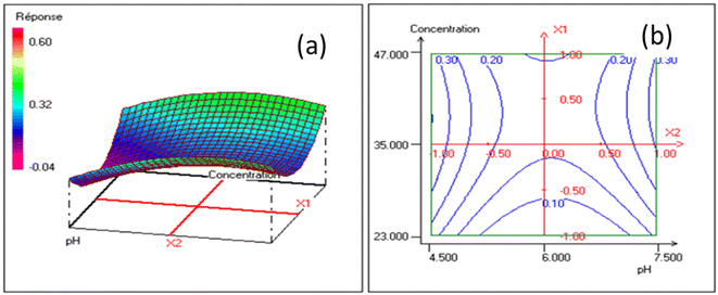Fig. 8 Response surfaces (a) and iso-response curves (b) showing the evolution of the content response for the concentration-pH.

4.2.3. Determination of optimal conditions for lead removal. In this study, the optimization of lead removal consists of determining the optimal values of lead concentration, solution pH, adsorbent mass, and contact time to maximize lead removal. The optimal conditions predicted by the model are recorded in Table 7. Those values confirmed the adequacy and validity of the model. Three replicate tests were performed under optimal conditions, with a removal rate of 99.028%. This value, being close to the one obtained by the model, shows a good correlation between the predicted and experimental values, demonstrating the eligibility of the model in its ability to predict the experimental responses. After examining the optimal conditions proposed by the Nemrodw analysis software, the efficiency of lead removal by shellfish is 98.138%.

Table 7 Optimal conditions for lead removal

Factors (Ui)				Rendement Y (%)
Initial concentration	pH	Mass of adsorbent	Contact time	Théorique	Experimental
47 mg L	4.5	0.2 g	125 min	98.138	99.028

---

5. Conclusions

This work investigates the ability of Corbula trigona shells to adsorb lead in an aqueous solution. The classical method was replaced by experimental design, which reduced the number of tests. The Plackett–Burman design (PBD) was used to identify important factors and quantify their effects on residual concentrations. It was found that the removal of lead on these biomaterials depends on the pH of the solution, mass of the adsorbent, contact time, and concentration of the pollutant in the solution, with contributions of 31.7%, 30.51%, 25.17%, and 12.44%, respectively. Subsequently, a composite central plane was used to optimize the lead removal process. It was found that the optimum conditions for removing up to 99.03% of the lead from an aqueous solution are: initial lead concentration of 47 mg L⁻¹, pH = 4.5, adsorbent mass of 0.20 g, and contact time of 125 min. The experimental lead removal rate (99.03%) obtained is quite similar to that of the established mathematical model (98.14%). The results of various characterisations confirmed that the adsorption of lead results in changes in morphology on the surface of the adsorbent, appearance of characteristic peaks in the spectra, and the appearance of lead in the chemical composition of adsorbents. Finally, this study showed that the valorization of Corbula trigona shell waste rich in calcium carbonate could be an effective adsorbent for remediating metal-contaminated wastewater and soil.

Conflicts of interest

No potential conflict of interest was reported by the author(s).

Acknowledgements

This work was carried out in the Laboratory Water Environment and Urban System at the University Paris Est Créteil. We thank the director and all the staff for welcoming us during our stay. Also we thank the Service of Cooperation and Cultural Action (SCAC)-Abidjan of the Embassy of France in Ivory Coast for the financing of my stay in France.

References

1. Y. H. A. Yapi, B. K. Dongui, A. Trokourey, Y. S. S. Barima, Y. Essis and P. Etheba, Int. j. biol. chem. sci., 2014, 8, 1281–1289.
2. O. Bamba, S. Pelede, A. Sako, N. Kagambega and M. Y. Miningou, J. des Sci., 2013, 13, 1–11.
3. A. H. Taylor, N. T. Cable, G. Faulkner, M. Hillsdon, M. Narici and A. K. Van Der Bij, J. Sports Sci., 2004, 22, 703–725.
4. F. Andriamasinoro, A. Hohmann, J.-M. Douguet and J.-M. Angel, Extr. Ind. Soc., 2020, 7, 1108–1120.
5. Y. Yapi, B. Dongui, A. Trokourey, Y. Barima, Y. Essis and P. Etheba, Int. j. biol. chem. sci., 2014, 8, 1281.
6. V. S. Kanwar, A. Sharma, A. L. Srivastav and L. Rani, Environ. Sci. Pollut. Res., 2020, 27, 44835–44860.
7. O. Karcioglu and B. Arslan, Poisoning in the Modern World: New Tricks for an Old Dog?, BoD – Books on Demand, 2019.
8. M. A. Salam, M. S. Makki and M. Y. Abdelaal, J. Alloys Compd., 2011, 509, 2582–2587.
9. K. Rathinam, P. Jayaram and M. Sankaran, Environ. Prog. Sustain., 2019, 38, S288–S297.
10. R. Zhou, Y. Xu, J. Shen, L. Han, X. Chen, X. Feng and X. Kuang, Sci. Rep., 2016, 6, 38930.
11. F. Fu and Q. Wang, J. Environ. Manage., 2011, 92, 407–418.
12. X. Cui, S. Fang, Y. Yao, T. Li, Q. Ni, X. Yang and Z. He, Sci. Total Environ., 2016, 562, 517–525.
13. M. M. Al-Ansari, H. Benabdelkamel, R. H. AlMalki, A. M. A. Rahman, E. Alnahmi, A. Masood, S. Ilavenil and K. C. Choi, Environ. Res., 2021, 199, 111240.
14. S. N. A. Abas, M. Ismail, L. Kamal and S. Izhar, World Appl. Sci. J., 2013, 28, 1518–1530.
15. J. suo Lu, T. ting Lian and J. feng Su, Res. Chem. Intermed., 2018, 44, 6011–6022.
16. A. A. Ahmed Eljiedi, A. Kamari, Sunardi and I. Fatimah, Arab J. Basic Appl. Sci., 2019, 26, 462–475.
17. M. Rezaei, N. Pourang and A. M. Moradi, Sci. Rep., 2022, 12, 1–20.
18. D. Alidoust, M. Kawahigashi, S. Yoshizawa, H. Sumida and M. Watanabe, J. Environ. Manage., 2014, 150, 103–110.
19. J. Polet, J. des Africanistes, 1995, 65, 93–109.
20. J. Goupy, Introduction aux plans d’expériences [Multimédia multisupport], Dunod, 2006.
21. M. Feinberg, La validation des méthodes d’analyse. Une approche chimiométrique de l’assurance qualité au laboratoire, Elsevier Mason SAS, 1996.
22. L. Addadi, D. Joester, F. Nudelman and S. Weiner, Chem. –Eur. J, 2006, 12, 980–987.
23. Y. Du, F. Lian and L. Zhu, Environ. Pollut., 2011, 159, 1763–1768.
24. A. Hossain, S. R. Bhattacharyya and G. Aditya, ACS Sustainable Chem. Eng., 2015, 3, 1–8.
25. C. Ketwong, S. Trisupakitti, C. Nausri and W. Senajuk, Naresuan Univ. Eng. J. Sci. Technol., 2018, 26, 61–70.
26. C. Martínez-García, B. González-Fonteboa, D. Carro-López and J. L. Pérez-Ordóñez, J. Clean. Prod., 2020, 269, 122343.
27. S. Safi, F. Karimzadeh and S. Labbaf, Mater. Sci. Eng. C, 2018, 92, 712–719.
28. T.-C. Hsu, J. Hazard. Mater., 2009, 171, 995–1000.
29. X. Xu, X. Hu, Z. Ding, Y. Chen and B. Gao, Chem. Eng. J., 2017, 308, 863–871.
30. L. Trakal, D. Bingöl, M. Pohořelý, M. Hruška and M. Komárek, Bioresour. Technol., 2014, 171, 442–451.
31. M. Singh, S. Vinodh Kumar, S. A. Waghmare and P. D. Sabale, Constr. Build. Mater., 2016, 112, 386–397.
32. K. Vijayaraghavan, A. Mahadevan, U. M. Joshi and R. Balasubramanian, J. Chem. Eng., 2009, 152, 116–121.
33. L. Fan, S. Zhang, X. Zhang, H. Zhou, Z. Lu and S. Wang, J. Environ. Manage., 2015, 156, 109–114.
34. X. Wang, S. Xia, L. Chen, J. Zhao, J. Chovelon and J. Nicole, J. Environ. Sci., 2006, 18, 840–844.
35. S. E. R. Mahunon, M. P. Aina, A. V. O. Akowanou, E. K. Kouassi, B. K. Yao, K. Adouby and P. Drogui, Environ. Sci. Pollut. Res., 2018, 25, 29219–29226.
36. E. K. Aziz, R. Abdelmajid, L. M. Rachid and E. H. Mohammadine, Arab J. Basic Appl. Sci., 2018, 25, 93–102.
37. S. M. Pourmortazavi, H. Sahebi, H. Zandavar and S. Mirsadeghi, Compos. B. Eng., 2019, 175, 107130.
38. R. Ahmad and A. Mirza, Groundw. Sustain. Dev., 2018, 7, 305–312.
39. D. Cao, X. Shi, H. Li, P. Xie, H. Zhang, J. Deng and Y. Liang, Ecotoxicol. Environ. Saf., 2015, 112, 231–237.
40. B. I. Okolo, E. O. Oke, C. M. Agu, O. Adeyi, K. Nwoso-Obieogu and K. N. Akatobi, Appl. Water Sci., 2020, 10, 201.
41. B. G. H. Briton, B. K. Yao, Y. Richardson, L. Duclaux, L. Reinert and Y. Soneda, Arab. J. Sci. Eng., 2020, 45, 7231–7245.
42. A. M. Joglekar, A. T. May, E. Graf and I. Saguy, Food product and development: From concept to the marketplace, 1987.
43. A. Salahi, I. Noshadi, R. Badrnezhad, B. Kanjilal and T. Mohammadi, J. Environ. Chem. Eng., 2013, 1, 218–225.
44. V. Javanbakht, H. Zilouei and K. Karimi, Int. biodeterior. biodegrad., 2011, 65, 294–300.

---