
 Open Access Article
 This Open Access Article is licensed under a Creative Commons Attribution-Non Commercial 3.0 Unported Licence
Extraction of interaction parameters from specular neutron reflectivity in thin films of diblock copolymers: an “inverse problem”†
Dustin
Eby
 a,
Mikolaj
Jakowski
a,
Valeria
Lauter
b,
Mathieu
Doucet
b,
Panchapakesan
Ganesh
*a,
Miguel
Fuentes-Cabrera
*a and
Rajeev
Kumar
*a
a,
Mikolaj
Jakowski
a,
Valeria
Lauter
b,
Mathieu
Doucet
b,
Panchapakesan
Ganesh
*a,
Miguel
Fuentes-Cabrera
*a and
Rajeev
Kumar
*a
aCenter for Nanophase Materials Sciences, Oak Ridge National Laboratory, Oak Ridge, TN-37831, USA. E-mail: ganeshp@ornl.gov; fuentescabma@ornl.gov; kumarr@ornl.gov
bNeutron Scattering Division, Oak Ridge National Laboratory, Oak Ridge, TN-37831, USA
First published on 10th March 2023
Abstract
Diblock copolymers have been shown to undergo microphase separation due to an interplay of repulsive interactions between dissimilar monomers, which leads to the stretching of chains and entropic loss due to the stretching. In thin films, additional effects due to confinement and monomer–surface interactions make microphase separation much more complicated than in that in bulks (i.e., without substrates). Previously, physics-based models have been used to interpret and extract various interaction parameters from the specular neutron reflectivities of annealed thin films containing diblock copolymers (J. P. Mahalik, J. W. Dugger, S. W. Sides, B. G. Sumpter, V. Lauter and R. Kumar, Interpreting neutron reflectivity profiles of diblock copolymer nanocomposite thin films using hybrid particle-field simulations, Macromolecules, 2018, 51(8), 3116; J. P. Mahalik, W. Li, A. T. Savici, S. Hahn, H. Lauter, H. Ambaye, B. G. Sumpter, V. Lauter and R. Kumar, Dispersity-driven stabilization of coexisting morphologies in asymmetric diblock copolymer thin films, Macromolecules, 2021, 54(1), 450). However, extracting Flory–Huggins χ parameters characterizing monomer–monomer, monomer–substrate, and monomer–air interactions has been labor-intensive and prone to errors, requiring the use of alternative methods for practical purposes. In this work, we have developed such an alternative method by employing a multi-layer perceptron, an autoencoder, and a variational autoencoder. These neural networks are used to extract interaction parameters not only from neutron scattering length density profiles constructed using self-consistent field theory-based simulations, but also from a noisy ad hoc model constructed previously. In particular, the variational autoencoder is shown to be the most promising tool when it comes to the reconstruction and extraction of parameters from an ad hoc neutron scattering length density profile of a thin film containing a symmetric di-block copolymer (poly(deuterated styrene-b-n-butyl methacrylate)). This work paves the way for automated analysis of specular neutron reflectivities from thin films of copolymers using machine learning tools.
Introduction
Neutron reflectometry1–3 (NR) has emerged as a unique characterization technique for studying thin polymer films due to its high spatial resolution (∼0.5 nm), non-destructive nature, and the sensitivity of neutrons to both isotopes and spin. When used in combination with other surface sensitive techniques such as X-ray reflectivity,1 time-of-flight secondary ion mass spectroscopy,4 ellipsometry, and transmission electron microscopy, NR provides detailed information about the structure of thin films along normal (specular NR) and in-plane directions (off-specular scattering). Due to the complicated data analysis of off-specular5 scattering, mainly specular NR has been extensively applied to various thin film systems since the 1980s. T. Russell and co-workers have applied NR in their pioneering work1 to study the surface enrichment of polymers in thin film blends, the adsorption of diblock copolymers on surfaces, and microphase separation in thin films of diblock copolymers. Since then, specular NR has been applied to many more polymeric systems such as polyelectrolyte brushes in solutions,6 block copolymer nanocomposites,7–12 disperse diblock copolymers,13,14 and ionic copolymer melts in the presence of applied electric fields.15T. Russell introduced and described ad hoc data analysis for multi-layers in his review of X-ray and neutron reflectivity in 1990,1 which contributed significantly to the widespread use of specular NR in studying polymeric systems. Nowadays, data analysis of specular NR (i.e. generating neutron scattering length density (SLD) profiles for a model and computing specular NR) can be done using publicly available packages such as the Refl1D,16 refnx,17 and BornAgain.18 By using these packages, typically the number and thickness of layers as well as roughness are varied to fit experimentally measured NR. Despite these advances, connecting NR to physics-based models has not been widely developed due to a number of complications. These complications include the selection of an appropriate physical model for the polymers under study, native oxide layers on substrates, and instrument resolution functions, which must be taken into account when fitting experimental reflectivity curves R(q) (q is the wave vector transfer perpendicular to the film surface). Furthermore, tackling the “inverse problems” still remains a challenge. These are (i) determining the SLD curves from the experimentally measured NR data and (ii) extracting the physical interaction parameters that produce those SLD curves. Both of these inversion problems remain unsolved and ill-posed because only reflected intensities are measured in most of the experiments, and the phase of reflected waves is not measured. Indeed, although it is possible to accurately determine the phase in an NR experiment using a known reference layer,19 a practical implementation of this method has not been established due to several obstacles, such as a significant increase in neutron scattering time required for experiments and difficulties associated with obtaining identical and reproducible reference layers. Similarly, when a SLD profile is constructed using linear combinations of different volume fraction profiles weighted appropriately by nuclear scattering cross-sections, sometimes different combinations of interaction parameters can lead to the same SLD profile (as shown in this work). Each of these inverse problems needs to be solved for facilitating the use of physics-based models for the interpretation of specular NR curves. This, in turn, will result in the discovery of unique information from NR experiments, which is not currently available. The importance of solving the inverse problem related to the loss of phase information in specular NR was identified as early as the late 1980s by T. Russell1 and G. Felcher.20 Specifically, T. Russell wrote, “It would be ideal if one could derive the scattering length density variation directly from the reflectivity profile. However, since the reflectivity profile is the square of the transform of the density profile, phase information is lost and calculating the potential or the scattering length density profile directly from R(kz,o) is not possible. This “inverse problem” has been and still is the major limitation of the reflectivity technique. It precludes an absolute determination of the scattering length density profile. The solution of this problem would constitute a major advance in the field and would remove some of the subjectivity associated with current data analysis”. These statements are still valid today on the 70th birthday of Prof. Russell, and in this work, we present our attempts to tackle a similar inverse problem arising in the extraction of interaction parameters from SLD curves. These parameters are present in a field-theoretic model, which is used to simulate volume fraction profiles of two components of a linear di-block copolymer in thin films. In turn, volume fraction profiles are used to construct the SLD. We plan to address the inverse problem stated by T. Russell in a future publication using the strategy presented in this work.
Previous attempts20,21 to solve the inverse problem related to the loss of phase in NR have used the Gel'fand–Levitan–Marchenko method,22 involving a numerical solution of an integral equation. Later on, the addition of reference layers and three NR measurements with polarized neutrons were proposed to invert reflectivity curves unambiguously.19,23 Although it is useful, the validity of the Gel'fand–Levitan–Marchenko method places constraints on the asymptotic behavior of SLDs, which is not known a priori. Similarly, the addition of a magnetic layer and additional measurements with polarized neutrons require alternative methods for converting NR into SLDs. In recent years, machine learning tools such as neural networks have been used to address the inverse problem.24–28 Neural networks can be trained to learn relations and then used to address the inverse problem. In this work, we use three different neural networks, i.e. a multi-layer perceptron, an autoencoder, and a variational autoencoder, to solve the inverse problem of extracting three interaction parameters from a SLD profile representing thin films containing linear and symmetric di-block copolymer chains. These thin films were studied in our previous works12,14 using self-consistent field theory (SCFT) of di-block copolymers and NR measurements. However, in our previous work, we constructed a SCFT-based model by carefully varying different parameters manually. Here, we have developed a suite of machine learning tools to extract the three interaction parameters of the SCFT from SLD, thereby expediting interpretation of specular NR using the SCFT.
For extracting interaction parameters, we focused on a thin film of the symmetric poly(deuterated styrene-b-n-butyl methacrylate) (poly(dS-b-BMA)) di-block copolymer. Thin films of these copolymers have been extensively studied by Lauter and coworkers7,8,10,12,14 using NR. In our previous work,12 we fitted experimental NR profiles from thin films of the lamellae forming poly(dS-b-BMA) di-block copolymer and constructed SLDs based on the SCFT model and an ad hoc multi-layer model. In other words, two models (almost similar to each other) were constructed12 to fit the same data, and additional information, such as phase information, was needed to determine which of these two models was better. With the goal of automating the process of estimating interaction parameters for the SCFT from SLDs, we herein use neural networks. Another goal is to identify a need to use a more realistic SCFT-based model13,14 with additional parameters such as dispersity of chain lengths, substrate properties etc. for interpreting the NR data. In this paper, we will show that indeed, our approach based on neural networks paves the way towards achieving these goals related to the inversion problem of going from NR data to SLD curves.
This paper is organized as follows: the Methods section provides a brief description of the SCFT-based model and describes in detail the three neural networks used in this work. The Results section shows the extracted parameters and discusses the results. We conclude with the Conclusions section.
Methods
SCFT-based simulations
We used self-consistent field theory (SCFT) to model the structure of thin films containing n A–B diblock copolymer (monodisperse and flexible) chains. The details of the SCFT and mapping the SCFT parameters for experimental poly(dS-b-BMA) are presented in our previous work.12 Briefly, two boundaries were included to represent silicon and air in the experimental set-up. A local incompressibility constraint was imposed on the system, so that at any location, the sum of the volume fractions of all the components (substrates, A and B) results in unity. A schematic of the system is shown in Fig. 1. Short-range pairwise interactions between different components were represented by Flory–Huggins χ parameters. Three parameters characterizing the interactions between different components were χA–BN and χp–kN = (χk–B − χk–A)N (k = Si, air), where N is the total number of statistical segments of the A and B chains, and subscripts p, Si, and air denote polymer, silicon and air, respectively. For comparisons with the experiments, A and B represent deuterated styrene (S) and n-butyl methacrylate (BMA), respectively. In this work, we have used χk–A = 0, so that χp–k = χk–B and negative values of these parameters will cause BMA to be localized at the boundary designated by k. Polyswift++![[thin space (1/6-em)]](https://www.rsc.org/images/entities/char_2009.gif) 29 was used to solve for volume fraction profiles of different components by solving a set of equations representing a saddle-point. As described in ref. 10 and 12, the spatial SLD profile was obtained using SLD(z) = SLDdPSϕA(z) + SLDPnBMAϕB(z) + SLDairϕa(z) + SLDSiO2ϕs(z), where z is normal to the substrate, SLDdPS = 6.19 × 10⁻⁶ Å−2, SLDPnBMA = 0.55 × 10⁻⁶ Å−2, SLDair = 0, and SLDSiO2 = 3.2 × 10⁻⁶ Å−2. It should be noted that the dPS used in the experiment10 was not fully deuterated, resulting in SLDdPS = 6.19 × 10⁻⁶ Å−2, which is lower than 6.45 × 10⁻⁶ Å−2 for fully deuterated PS.30
29 was used to solve for volume fraction profiles of different components by solving a set of equations representing a saddle-point. As described in ref. 10 and 12, the spatial SLD profile was obtained using SLD(z) = SLDdPSϕA(z) + SLDPnBMAϕB(z) + SLDairϕa(z) + SLDSiO2ϕs(z), where z is normal to the substrate, SLDdPS = 6.19 × 10⁻⁶ Å−2, SLDPnBMA = 0.55 × 10⁻⁶ Å−2, SLDair = 0, and SLDSiO2 = 3.2 × 10⁻⁶ Å−2. It should be noted that the dPS used in the experiment10 was not fully deuterated, resulting in SLDdPS = 6.19 × 10⁻⁶ Å−2, which is lower than 6.45 × 10⁻⁶ Å−2 for fully deuterated PS.30
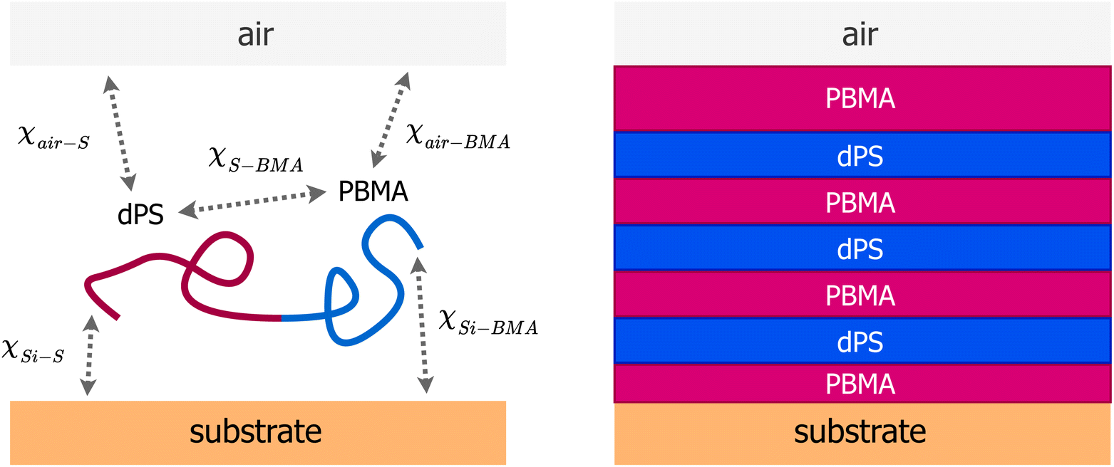 | ||
| Fig. 1 (Left) A schematic of the system showing the substrate (silicon), diblock copolymer chain, and interaction parameters. All pairwise interactions considered in the SCFT-based model are represented by the Flory–Huggins χ parameters. SCFT was used to simulate different morphologies in the film of a known thickness by varying three parameters χS–BMA, χair–BMA − χair–S and χSi–BMA − χSi–S. (Right) Schematic of the morphology in the thin film studied in this work and previously by us12 using neutron reflectivity, which exhibits three alternating strongly segregated domains of PBMA-dPS-PBMA. | ||
Data creation: SLD profiles vs. the three Flory–Huggins χ parameters
SLD profiles were constructed from the volume fraction profiles obtained after solving the SCFT equations for a fixed film thickness. The SCFT equations were solved on a Cartesian three-dimensional grid with Nx = Ny = 16, and Nz = 96 collocation points along x, y, and z, respectively, with a uniform grid spacing of Δx = Δy = Δz = 0.145. All the lengths were made dimensionless using the radius of gyration of the diblock copolymer chains, which was taken to be Rgo = 136.47 Å, based on our previous work.12 In addition, N = 198 and the chain contour step Δs = 0.01 was used for solving the equations for chain propagators. For generating the SLD profiles, volume fractions were averaged along x and y. This way, a total of 5942 SLD profiles were generated with χA–B ≡ χS–BMA ranging in value from 0.05 to 0.20, χp–Si ranging from −0.6 to 0.6, and χp–air also ranging from −0.6 to 0.6. These SLD profiles were stored as 2 × 97 matrices, which were indexed along with their corresponding χ input parameters to form our dataset.The experimental measurement12 on the symmetric poly(dS-b-nBMA) film revealed three strongly segregated domains of PBMA-dPS-PBMA (cf.Fig. 1). Such strong segregation of microphase separated domains places a bound on the lowest value of the interaction parameter χS–BMA. Below this value, the domains exhibit mixing of dPS and PBMA. In addition, we have to impose an upper bound on χS–BMA as the SLD profiles do not change significantly beyond this value. So, we analyzed SLD profiles for a narrower range of values lying in the ranges 0.08 ≤ χS–BMA ≤ 0.11 and 0.07 ≤ χS–BMA ≤ 0.12 for the multi-layer perceptron (MLP) and autoencoders, respectively. After this, our dataset consisted of 1931 simulated SLD curves and their input χ parameters. We split this dataset into 3 sets, a training set (70%), a validation set (15%), and a testing set (15%).
NR is sensitive to the thickness and roughness at the boundary of both surfaces (i.e., polymer–air and polymer–silicon). As we do not simulate these details of the boundary layers and we want to extract parameters from the SLD profiles, we used the SLD profiles corresponding to the interior of the films and discarded SLD data below z = 251 Å and above z = 1680 Å, reducing our SLD matrices to 2 × 72. The SLD curves were then normalized to have x and y scales from 0 to 1. Similarly, an oxide layer was added to the SCFT-based SLD profiles before computing reflectivities. Simulation failures appeared as straight horizontal lines, so the dataset was checked and cleaned of these poor data points.
Artificial neural networks (ANNs)
In this paper, three different ANN architectures were used to tackle the inverse problem. The first architecture was based on a multi-layer perceptron31 (MLP), shown schematically in Fig. 2. The MLP was trained to learn the relationship between SCFT-generated SLD profiles and χ parameters. It could be seen that even though the MLP was capable of predicting accurately the χ parameters for the SCFT-generated SLD curves, it produced unphysical χ parameters for an experimental SLD curve. To overcome this issue, we constructed an ANN architecture comprising an autoencoder (AE) and an MLP. This architecture was inspired by the work of Routh et al.,32 who used an AE and MLP to predict physical descriptors from X-ray absorption near edge structure (XANES) spectra. The AE-MLP hybrid model architecture is shown in Fig. 3. The AE was composed of two ANNs, the encoder and the decoder. The encoder took in the SCFT SLD curves and compressed them into vectors in a multidimensional “latent” space. The decoder took in vectors from this latent space and regenerated the corresponding SLD curves. The AE was trained until the SLD curves generated by the decoder resembled the corresponding SCFT input. This was done by generating a loss function, where the output of any given pass is compared against its true input, and then minimizing this loss. Once the AE was trained, the latent space vectors contained the most important information associated with the input SCFT SLD curves. In this approach, for each SCFT SLD curve, there is a vector in the latent space, and for each vector, there is also a corresponding set of χ parameters. Next, the MLP was trained on the relationship between the latent space and the χ parameters. The reasoning for using the MLP is follows: as the latent space can have a smaller dimension than the dataset composed of SCFT SLD curves, it should be more efficient to train the MLP on the relationship between the latent space and the χ parameters than to train it on the relationship between SCFT SLD curves and χ parameters, as we did initially. Subsequently, we reasoned that it might be possible to use the AE-MLP architecture to accurately predict the χ parameters of an experimental SLD curve. Unfortunately, we did not succeed in achieving the latter because, as it will be seen, the decoder was incapable of regenerating the experimental SLD curve accurately. The reason for this is rooted in the sparsity of the latent space: the mapping of SCFT SLD curves into the latent space resulted in 4 well-separated clusters, none of which contained the point associated with the experimental SLD curve. To solve this issue and focus mainly on reproducing the experimental SLD curve, we replaced the AE with a variational autoencoder, VAE,33 which is a probabilistic extension of an AE. In a VAE, an additional term is added to the loss function to achieve regularization of the latent space, thereby making it continuous and complete. The VAE architecture is shown in Fig. 4. The decoder of the VAE was capable of regenerating an experimental SLD curve accurately. Below, we describe the components of each architecture.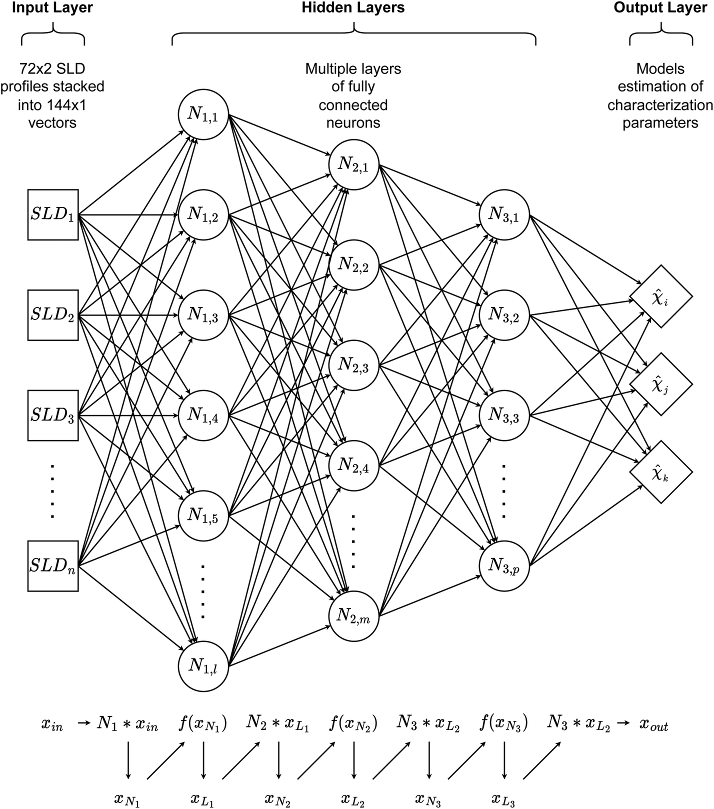 | ||
| Fig. 2 Schematic representation of the multi-layer perceptron (MLP) architecture. It takes SLD curves as inputs and outputs the corresponding three Flory–Huggins parameters. Here, f(x) is an activation function. | ||
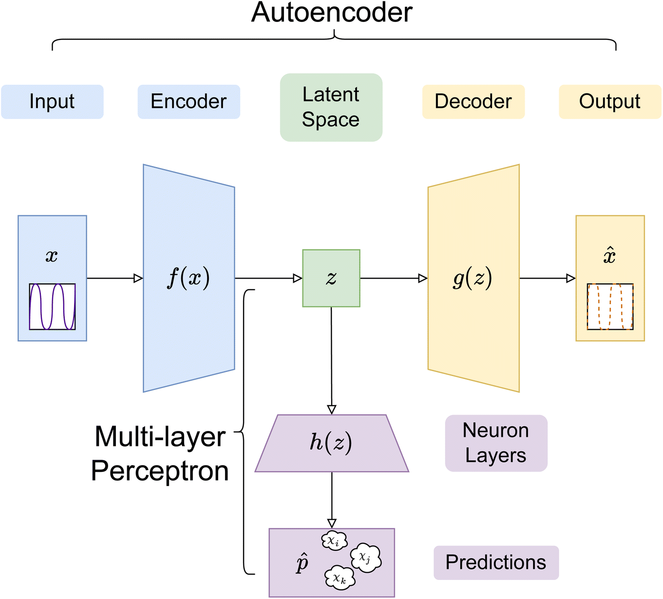 | ||
Fig. 3 Schematic representation of the AE-MLP architecture. The encoder, f(x), takes SLD curves, x, as inputs and compresses them into the latent space, z. The decoder, g(z), generates SLD curves ![[x with combining circumflex]](https://www.rsc.org/images/entities/i_char_0078_0302.gif) which, when the AE is properly trained, resemble x. The multi-layer perceptron (MLP), h(z), takes vectors in z as inputs and outputs the corresponding three Flory–Huggins χ parameters. which, when the AE is properly trained, resemble x. The multi-layer perceptron (MLP), h(z), takes vectors in z as inputs and outputs the corresponding three Flory–Huggins χ parameters. | ||
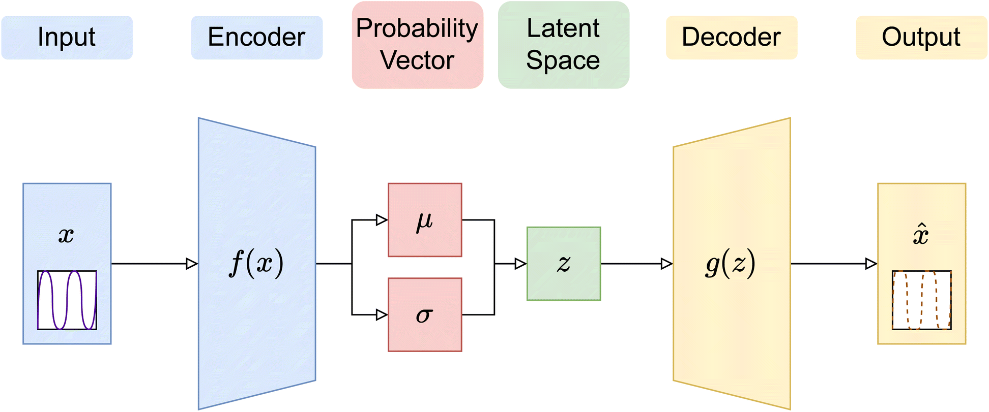 | ||
| Fig. 4 Diagram of a variational autoencoder (VAE) structure, with the encoding outputs as Bayesian probability vectors shown. All other details are the same as in Fig. 3. | ||
All three ANNs were coded in PyTorch. In the MLP architecture, as shown in Fig. 2, the MLP contained 6 dense layers of 400, 300, 200, 100, 80, and 30 neurons, with all layers using the ReLU as the activation function. The MLP was trained over 800 epochs on 16-sample batches of training datasets using the mean squared error (MSE) loss and the AdamW optimizer with a learning rate of 0.0001.
In the AE-MLP architecture, as shown in Fig. 3, the encoder of the AE was composed of 2 dense layers of 96 and 64 neurons each, with ReLU non-linear activation. The decoder had an identical number of layers to the encoder, but in reverse order. The AE was trained over 800 epochs with 16-sample batches, using the MSE loss and the AdamW optimizer with a learning rate of 0.0001. The effect that changing the dimensionality of the latent space, nl, had on the results was investigated by assigning the values 2, 3, and 4 to nl. The MLP composition in the AE-MLP network was identical to the one described in the preceding paragraph.
Given that we are modeling a physical system, the latent space is expected to have some regular structures, which are continuous and complete. In an AE, the continuity and completeness of latent space projection are not guaranteed, since there is no explicit term in the loss function (i.e., mean square error) that ensures projection to random regions of the latent space, hindering construction of meaningful latent space representations. In this work, the encoder in a VAE was set up such that the last layer created probability vectors in the latent space, which can then be regularised using a Kullback–Leibler (KL) divergence term, in addition to the usual cross-entropy loss in an AE between the input and output vectors, to cover defined and predictably sized continuous regions. Thus, in the VAE, the latent vectors used to decode are not just singular points, but also samples from the distributions created by each encoding.
Results
In this section we describe how we have used SCFT SLD data to train the ANNs described above and use them to extract physical descriptors (i.e. the χ parameters) or reproduced SLD profiles. We started with the experimental NR curve obtained in ref. 10. This curve is referred to as “Experimental data” in Fig. 5a. In our previous work,12 we showed that the SCFT-based simulations capture long-wavelength physics correctly and computed NR using the simulations. To show this, we first added a semi-infinite layer of silicon (SLDSi = 2.07 × 10⁻⁶ Å−2) and a finite layer of silicon oxide to a simulated SLD curve. Then we varied SLDs to fit the experimental data. The resultant curve is denoted as “Fit: SCFT informed” in Fig. 5b. The resultant NR curve is denoted as “Fit: SCFT informed” in Fig. 5a. This curve captures well the long-wavelength behaviour of the “Experimental data”.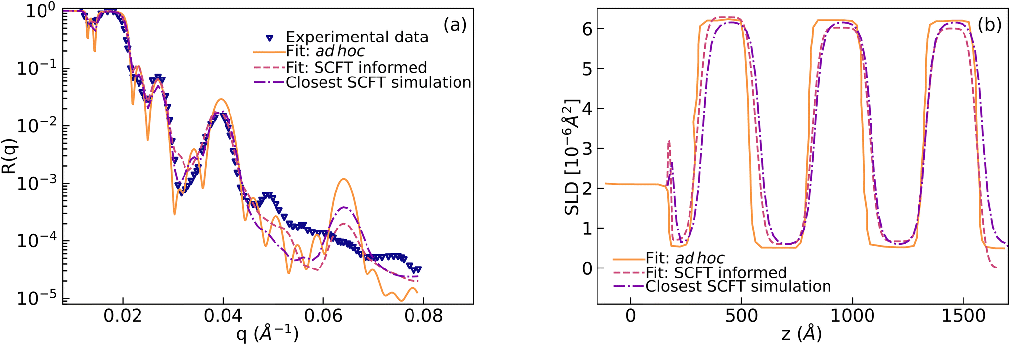 | ||
| Fig. 5 (a) Measured neutron reflectivity (labeled as “Experimental data”) vs. wavevector (q) for the film containing poly(dS-b-BMA). Two models containing multi-layers were constructed to fit the experimental data. The first model was constructed in an ad hoc way10,12 (“Fit: ad hoc”) and the second model was built using information obtained from the SCFT for the number and thickness of microphase-separated domains (“Fit: SCFT informed”). Reflectivity computed from the SLD profile which was constructed from the SCFT simulation using the three chi parameters closest to the predicted parameters is also shown (“Closest SCFT simulation”). (b) The SLD profiles for computing these reflectivities. | ||
After this, we used the MLP for extracting the Flory–Huggins χ parameters for the “Fit: SCFT informed” SLD curve. For this purpose, we trained the MLP on a set of SCFT-generated SLD curves and associated χ values. After training, we tasked the MLP with predicting the χ values for a set of SCFT curves, which were not used during training (this set is known as the test set in the ML jargon). The MLP predicted χ values for the test set are shown against the true values in Fig. 6. Clearly, the MLP was capable of predicting accurately the χ parameters. This MLP was subsequently used to predict the χ parameters for the “Fit: SCFT informed” SLD curve shown in Fig. 5b. The results were χS–BMA = 0.11, χp–Si = −0.42, and χp–air = −0.075, and are shown in Fig. 6 as “orange dots”. These values are qualitatively correct, as they lead to the localization of PBMA at both the silicon and air surfaces. However, these values are outside the original distribution of χ parameters: they are not parts of the χ set associated with the SCFT SLD-generated curves, shown as black dots in Fig. 6. The triplets of “black dots” that approach the “orange dots” most closely were determined to be χS–BMA = 0.12, χp–Si = −0.42, and χp–air = −0.083. For these values, the corresponding SCFT SLD curve and related NR curves are referred to as the “Closest SCFT simulation” in Fig. 5b and Fig. 5a, respectively. These results illustrate the degeneracy of the solution when extracting physical parameters from NR curves: similar SLD curves can have different χ physical descriptions that produce different NR curves.
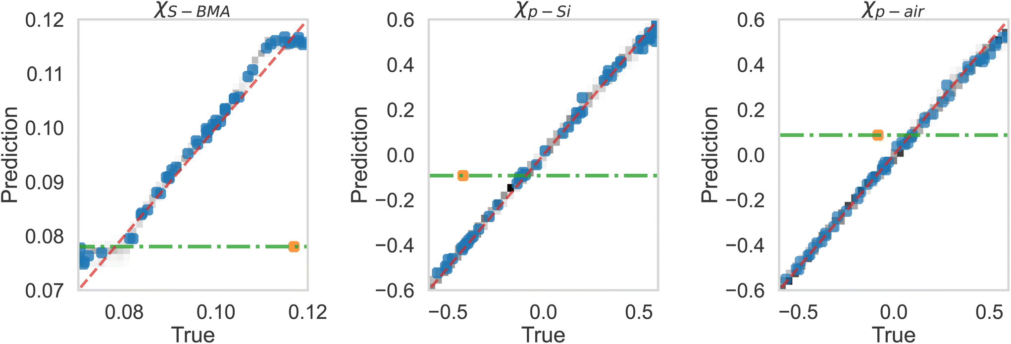 | ||
| Fig. 6 True vs. predicted values from the MLP of simulation (black dots) data, along with the best estimations of the three parameters for the “Fit: SCFT informed” curve shown in Fig. 5 as True (orange dot). Current best estimations for the parameters corresponding to “Fit: ad hoc” in Fig. 5 are also shown. These estimates are at the intersection of the horizontal green lines and dashed red lines. | ||
Lauter et al.10 were able to construct another SLD curve that produced a NR profile that captured the long-wavelength behavior. This SLD curve and the corresponding NR profile are shown in Fig. 5b and Fig. 5a, respectively, and denoted as “Fit: ad hoc”. To determine the χ parameters for this ad hoc constructed SLD curve, we used the MLP. The values found were χS–BMA = 0.078, χp–Si = −0.092, and χp–air = +0.087 (see the green lines in Fig. 6), which are qualitatively incorrect as a positive value of the parameter χp–air implies that PBMA should be repelled from the air and this is non-physical.
To understand why an MLP trained on SCFT SLD generated curves was not capable of predicting physically meaningful χ parameters for the “Fit: ad hoc” SLD curve, we analyzed the last hidden layer of the MLP. This layer has 30 neurons, and to visualize its output, we used the t-distributed Stochastic Neighbor Embedding (t-SNE) method. The t-SNE method approximates an isometry between a thirty-dimensional space and a two-dimensional space (the distance between any two points in the 30 dimensional space is roughly the same as the distance between their images in the two dimensional space). The t-SNE plot is shown in Fig. 7, and it is clear that the SCFT SLD curves are clustered into four groups. The groups are shown in a column on the right side of Fig. 7, and from top to bottom they correspond to the following monomer configurations:
• Three microphase separated domains of dPS–PBMA–dPS, with dPS interfacing with both the substrate and air.
• Three microphase separated domains of PBMA–dPS–PBMA, with PBMA on the substrate side and a dPS domain on the air side.
• Three microphase separated domains of PBMA–dPS–PBMA, with PBMA interfacing with the substrate and air.
• Three microphase separated domains of dPS–PBMA–dPS, with dPS enriching the substrate and a PBMA domain at the air side.
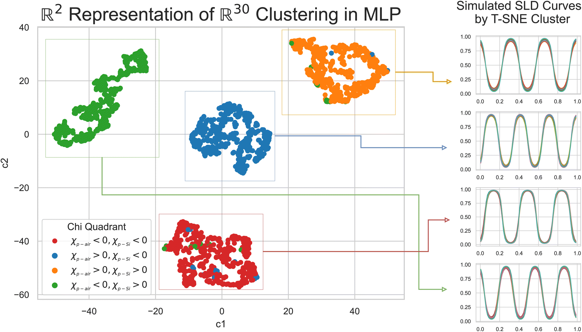 | ||
| Fig. 7 Visualization of the latent space in the last layer of a multi-layer perceptron (MLP), and the clustering of SLD curves within. The red and orange clusters have dots of different colors representing the SLD curves, which do not belong to these clusters (seen in the right panels). These dots imply that the categorization of the data into the four clusters is not perfect and there are some exceptions. Silicon substrate and air are at 0 and 1, respectively, on the rescaled axes of the SLD curves. | ||
The clustering observed is of course a consequence of the choices made when generating the SLD curves with the SCFT. In particular, the number of microphase-separated domains was fixed at three due to the parameterization used in the SCFT simulations. In Fig. 7, we also show the χ parameter ranges associated with each cluster. The t-SNE analysis showed that the clusters associated with the SCFT SLD curves were tight, with high levels of sparsity in between them. This explains why the MLP was not capable of predicting accurately the χ parameter for the ad-hoc model: the “Fit: ad hoc” SLD curve may lie in the sparse region between the clusters in Fig. 7, where the MLP was not trained. In the following, we show that this was indeed true.
While the physically simulated model is constrained to lie in one of the four clusters, the experimental curve could lie in the sparse region because the complete physical model describing it may be in a higher dimension than the three dimensions used to build the simulated data i.e., the complete physical model might require more than the three interaction parameters. Using the AE-MLP architecture, we can identify the “true” dimensionality, and interpret its physical meaning. This would effectively allow us to also extend our physical model to capture the missing physics in the experimental data. For such purposes, we trained the AE with a set of SCFT SLD curves and the dimension of the latent space being 2, 3 or 4. The latent space with a dimension nl = 2 is shown in Fig. 8(left), and it is seen that the clustering observed resembles that in Fig. 7. The latent point corresponding to the SLD curve “Fit: ad hoc” is placed in between two of the clusters (see Fig. 8(left). Therefore, as can be seen in Fig. 9(left), the decoder of the AE is unable to reproduce the SLD “Fit: ad hoc” curve accurately. In fact, it seems that the decoder attempts to draw an average of the two SLD curves associated with the nearest two clusters. The reason for this is once again related to the fact that the “Fit: ad hoc” SLD curve is not represented by any of the curves in the set used to train the AE.
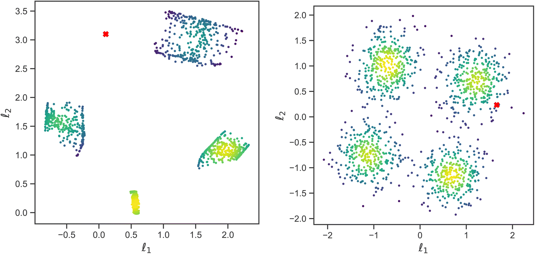 | ||
| Fig. 8 Plot showing latent space representation of a traditional autoencoder (left) versus a variational autoencoder (right). Both have latent dimensionality nl = 2, and l1 and l2 are latent space variables. The VAE has Kullback–Liebler divergence β = 1. Red crosses correspond to the SLD curve labeled as “Fit: ad hoc” in Fig. 5b. | ||
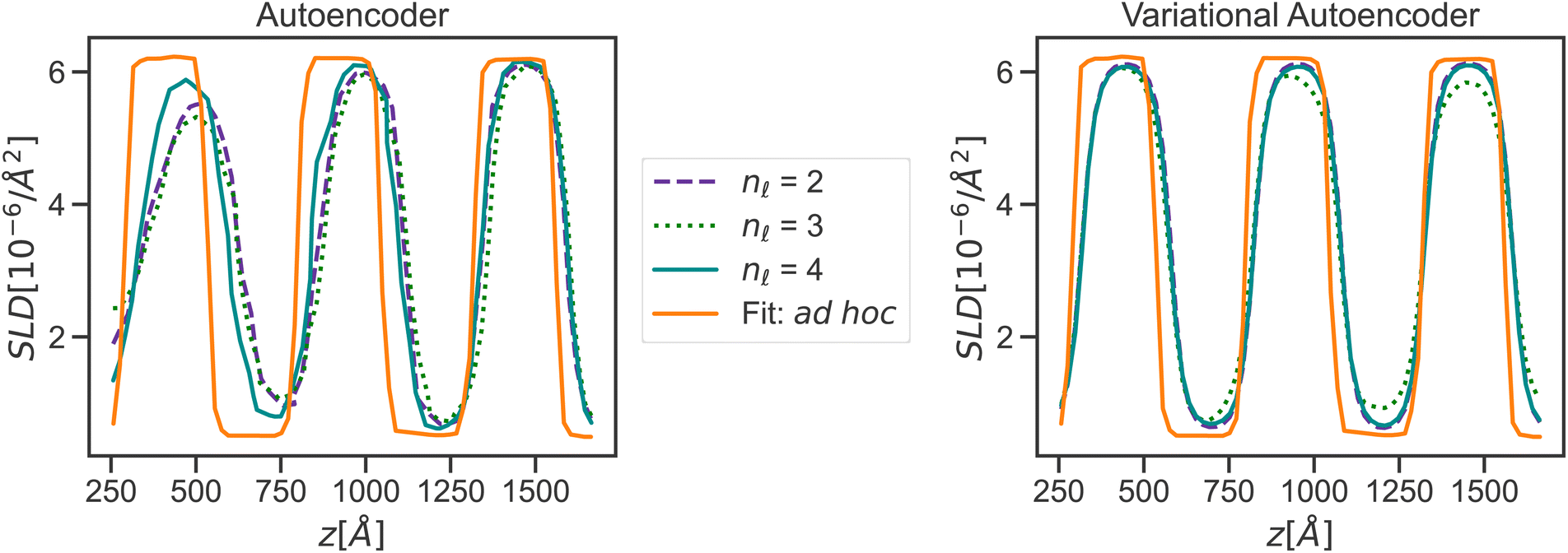 | ||
| Fig. 9 Reconstruction of an experimental curve (“Fit: ad hoc”, which is the same as shown in Fig. 5) from an autoencoder (left) and variational autoencoder (right) across multiple latent space dimensionalities. | ||
Despite this, in an effort to determine the optimal latent space dimension needed to capture the most important features of the SCFT SLD curves, we trained the MLP on the relationship between the latent space and the corresponding χ parameters. The MLP predicted χ values vs. the true ones are shown in Fig. 10 for nl = 2, 3, 4. Interestingly, the accuracy of the prediction increases with nl, revealing that a nl = 4 produces near-optimal retention of SCFT SLD information. This leads to an intriguing hypothesis: the complete physical model describing the NR data correctly might lie in a higher dimension than the three dimensions used to build the simulated data. This hypothesis will be probed in more detail in future studies.
 | ||
| Fig. 10 Truth vs. prediction of the three χ parameters for a hybrid model with an autoencoder and an MLP while varying the number of latent space parameters, nl = 2, 3, and 4 in the top, middle, and bottom rows, respectively. | ||
Increasing nl beyond 4 did not solve the issue with the decoder not being able to reconstruct the SLD curve. At this point, however, we only focused on improving reconstruction with the decoder of the “Fit: ad hoc” SLD curve. For this purpose, we explored whether using a VAE will improve reconstruction. As we did with the AE, we also trained the VAE with the same set of the SCFT SLD curves. During training, nl was also varied and had values of 2, 3, and 4. The latent space for nl = 2 is shown in Fig. 8(right). Four major clusters were still observed, but now the transition between these clusters was much smoother than the transition seen in Fig. 8(left) for the latent space of the AE. Furthermore, the latent point corresponding to the “Fit: ad hoc” SLD curve now lies in one of the transition regions. As a consequence, and as shown in Fig. 9(right), the decoder of the VAE was capable of reproducing the “Fit: ad hoc” curve in a better way. This points out that indeed a physical model such as the one based on the SCFT needs to have more than three parameters to describe the NR data correctly. These additional parameters may include the dispersity of the chain lengths, which leads to an increase in the thickness of the microphase separated domains. Nevertheless, this work shows that VAEs can be used to identify a need for an improved physical model.
Conclusions
This work provides a set of neural networks for extracting interaction parameters from neutron SLD profiles obtained for thin films of diblock copolymers. These networks consist of a multi-layer perceptron (MLP), an autoencoder (AE) combined with a MLP, and a variational autoencoder (VAE). All three networks were trained on the SLD profiles generated by SCFT-based simulations for a given film thickness, while varying three Flory–Huggins interaction parameters. The MLP and the AE-MLP were successful in learning the relationships between the SCFT SLD curves and the corresponding three Flory–Huggins χ parameters, but they were not able to predict correctly the χ parameters for an experimental SLD curve. The reasons for this were: (i) the experimental SLD curve lay outside the distribution of SCFT curves used during training; and (ii) the sparsity and clustering of the SCFT SLD curves. This sparsity resulted from the underlying physics of microphase separation in di-block copolymers, which enforced a fixed number of microphase separated domains for a given film thickness and chain connectivity, and led to alternative domains containing different monomers. It was observed that small deviations of the experimental SLD curves from the SCFT ones caused misinterpretation of interaction parameters. The VAE permits the construction of continuous and complete latent space representations, which allowed experimental data that fell in regions where SCFT data did not exist to be accounted for. As a consequence, the decoder of the VAE was capable of reproducing an experimental SLD curve, something that the decoder of the AE was incapable of doing. The fact that the VAE showed better reproducibility of the SLD experimental curve when the dimension of the latent space was 4 suggests that the physical model that better represents the experimental data might consist of more than 3 parameters. This will be investigated in future studies as it presents an exciting opportunity for interpreting experimental SLD curves. Overall, the machine learning techniques used here provide a practical approach to solve the problem of neutron reflectivity inversion to SLD and even interaction parameters. Indeed, this work not only outlines the feasibility of a machine learning-based approach to the extraction of interaction parameters from neutron SLD curves, but also more broadly demonstrates the feasibility of machine learning models to tackle the inverse problem in general.34 The insights from the models in this work move us closer towards the application of machine learning models in the analysis of off-specular scattering,35 which is currently a difficult task. While the models shown in this paper demonstrate the capabilities of our approach, more work and refinement are still needed to generate a model with the predictive accuracy required for researchers to adopt this framework.Data availability
All of the data including the SCFT simulations and scripts for the ANNs, AEs, and VAEs are available at https://github.com/miguel-fc/NR-SCFT-ML.Author contributions
D. E., M. J., M. D., and M. F-C. contributed to the development of Python packages, the multi-layer perceptron and autoencoders. V. L., M. D., and R. K. contributed to conceptualization, the initial implementation of neural networks, and the SCFT-based analysis of the experimental data. P. G. contributed to interpretation and discussion about the VAE usage. All authors contributed to writing of the manuscript.Conflicts of interest
Authors declare no conflict of interest.Acknowledgements
Analysis of NR using machine learning tools was supported by the Center for Nanophase Materials Sciences, (CNMS), which is a US Department of Energy, Office of Science User Facility at Oak Ridge National Laboratory. DE and MJ acknowledge the sponsorship of this research by the US Department of Energy, Office of Science through the Science Undergraduate Laboratory Internship (SULI) and the management of this program through the ORISE. RK acknowledges discussions about NR with Dr James Browning, Dr Hanyu Wang, Dr Brad Lokitz, and Dr John F. Ankner. This research used the resources of the Compute and Data Environment for Science (CADES) at the Oak Ridge National Laboratory, which are supported by the Office of Science of the U.S. Department of Energy under contract no. DE-AC05-00OR22725. This research used resources at the Spallation Neutron Source, a Department of Energy Office of Science User Facility operated by the Oak Ridge National Laboratory.References
- T. Russell, X-ray and neutron reflectivity for the investigation of polymers, Mater. Sci. Rep., 1990, 5, 171–271 CrossRef CAS.
- J. Ankner and G. Felcher, Polarized-neutron reflectometry, J. Magn. Magn. Mater., 1999, 200, 741–754 CrossRef CAS.
- J. Daillant and A. Gibaud, X-ray and Neutron Reflectivity: Principles and Applications, Springer, 2008, vol. 770 Search PubMed.
- A. H. Mah, T. Laws, W. Li, H. Mei, C. C. Brown, A. Ievlev, R. Kumar, R. Verduzco and G. E. Stein, Entropic and enthalpic effects in thin film blends of homopolymers and bottlebrush polymers, Macromolecules, 2019, 52, 1526–1535 CrossRef CAS.
- S. K. Sinha, E. B. Sirota, S. Garoff and H. B. Stanley, X-ray and neutron scattering from rough surfaces, Phys. Rev. B: Condens. Matter Mater. Phys., 1988, 38, 2297–2311 CrossRef PubMed.
- J. P. Mahalik, Y. B. Yang, C. Deodhar, J. F. Ankner, B. S. Lokitz, S. M. Kilbey, B. G. Sumpter and R. Kumar, Monomer volume fraction profiles in pH responsive planar polyelectrolyte brushes, J. Polym. Sci., Part B: Polym. Phys., 2016, 54, 956–964 CrossRef CAS.
- V. Lauter-Pasyuk, H. Lauter, D. Ausserre, Y. Gallot, V. Cabuil, E. Kornilov and B. Hamdoun, Effect of nanoparticle size on the internal structure of copolymer–nanoparticles composite thin films studied by neutron reflection, Phys. B, 1997, 241, 1092–1094 CrossRef.
- V. Lauter-Pasyuk, H. Lauter, D. Ausserre, Y. Gallot, V. Cabuil, B. Hamdoun and E. Kornilov, Neutron reflectivity studies of composite nanoparticle–copolymer thin films, Phys. B, 1998, 248, 243–245 CrossRef CAS.
- S. Lefebure, V. Cabuil, D. Ausserré, F. Paris, Y. Gallot and V. Lauter-Pasyuk, in Lamellar Composite Magnetic Materials, ed. G. J. M. Koper, D. Bedeaux, C. Cavaco and W. F. C. Sager, Steinkopff, Darmstadt, 1998, pp. 94–98 Search PubMed.
- V. Lauter-Pasyuk, H. J. Lauter, G. P. Gordeev, P. Muller-Buschbaum, B. P. Toperverg, M. Jernenkov and W. Petry, Nanoparticles in block-copolymer films studied by specular and off-specular neutron scattering, Langmuir, 2003, 19, 7783–7788 CrossRef CAS.
- V. Lauter, P. Muller-Buschbaum, H. Lauter and W. Petry, Morphology of thin nanocomposite films of asymmetric diblock copolymer and magnetite nanoparticles, J. Phys.: Condens. Matter, 2011, 23, 254215 CrossRef PubMed.
- J. P. Mahalik, J. W. Dugger, S. W. Sides, B. G. Sumpter, V. Lauter and R. Kumar, Interpreting neutron reflectivity profiles of diblock copolymer nanocomposite thin films using hybrid particle-field simulations, Macromolecules, 2018, 51, 3116–3125 CrossRef CAS.
- R. Kumar, B. S. Lokitz, S. W. Sides, J. Chen, W. T. Heller, J. F. Ankner, J. F. Browning, I. Kilbey, S. Michael and B. G. Sumpter, Microphase separation in thin films of lamellar forming polydisperse di-block copolymers, RSC Adv., 2015, 5, 21336–21348 RSC.
- J. P. Mahalik, W. Li, A. T. Savici, S. Hahn, H. Lauter, H. Ambaye, B. G. Sumpter, V. Lauter and R. Kumar, Dispersity-driven stabilization of coexisting morphologies in asymmetric diblock copolymer thin films, Macromolecules, 2021, 54, 450–459 CrossRef CAS.
- J. W. Dugger, W. Li, M. Chen, T. E. Long, R. J. L. Welbourn, M. W. Skoda, J. F. Browning, R. Kumar and B. S. Lokitz, Nanoscale resolution of electric-field induced motion in ionic diblock copolymer thin films, ACS Appl. Mater. Interfaces, 2018, 10, 32678–32687 CrossRef CAS PubMed.
- P. Kienzle, J. Krycka, N. Patel and I. Sahin, Refl1D (version 0.8. 15)[computer software], University of Maryland, College Park, MD. [Google Scholar], 2022 Search PubMed.
- A. R. Nelson and S. W. Prescott, refnx: neutron and X-ray reflectometry analysis in Python, J. Appl. Crystallogr., 2019, 52, 193–200 CrossRef CAS PubMed.
- G. Pospelov, W. Van Herck, J. Burle, J. M. Carmona Loaiza, C. Durniak, J. M. Fisher, M. Ganeva, D. Yurov and J. Wuttke, BornAgain: Software for simulating and fitting grazing-incidence small-angle scattering, J. Appl. Crystallogr., 2020, 53, 262–276 CrossRef CAS PubMed.
- C. F. Majkrzak and N. F. Berk, Exact determination of the phase in neutron reflectometry by variation of the surrounding media, Phys. Rev. B: Condens. Matter Mater. Phys., 1998, 58, 15416–15418 CrossRef CAS.
- G. Felcher, Thin Film Neutron Optical Devices: Mirrors, Supermirrors, Multilayer Monochromators, Polarizers, and Beam Guides, 1989, pp. 2–9 Search PubMed.
- M. V. Klibanov, P. E. Sacks and A. V. Tikhonravov, The phase retrieval problem, Inverse Probl., 1995, 11, 1 CrossRef.
- K. Chadan and P. C. Sabatier, Inverse Problems in Quantum Scattering Theory, Springer Science & Business Media, 2012 Search PubMed.
- V. de Haan, A. van Well, P. Sacks, S. Adenwalla and G. Felcher, Toward the solution of the inverse problem in neutron reflectometry, Phys. B, 1996, 221, 524–532 CrossRef CAS.
- M. Doucet, R. K. Archibald and W. T. Heller, Machine learning for neutron reflectometry data analysis of two-layer thin films, Mach. Learn.: Sci. Technol., 2021, 2, 035001 Search PubMed.
- J. M. C. Loaiza and Z. Raza, Towards reflectivity profile inversion through artificial neural networks, Mach. Learn.: Sci. Technol., 2021, 2, 025034 Search PubMed.
- A. Greco, V. Starostin, A. Hinderhofer, A. Gerlach, M. W. Skoda, S. Kowarik and F. Schreiber, Neural network analysis of neutron and x-ray reflectivity data: pathological cases, performance and perspectives, Mach. Learn.: Sci. Technol., 2021, 045003 Search PubMed.
- A. Greco, V. Starostin, E. Edel, V. Munteanu, N. Rußegger, I. Dax, C. Shen, F. Bertram, A. Hinderhofer and A. Gerlach, et al., Neural network analysis of neutron and X-ray reflectivity data: automated analysis using mlreflect, experimental errors and feature engineering, J. Appl. Crystallogr., 2022, 55, 362–369 CrossRef CAS PubMed.
- H. Aoki, Y. Liu and T. Yamashita, Deep learning approach for an interface structure analysis with a large statistical noise in neutron reflectometry, Sci. Rep., 2021, 11, 1–9 CrossRef PubMed.
- https://www.txcorp.com .
- M. J. Park, K. Char, J. Bang and T. P. Lodge, Order-disorder transition and critical micelle temperature in concentrated block copolymer solutions, Macromolecules, 2005, 38, 2449–2459 CrossRef CAS.
-
A. Ivakhnenko and V. Lapa, Cybernetic Predicting Devices. CCM Information Corporation, First Working Deep Learners with Many Layers, Learning Internal Representations, 1965 Search PubMed.
- P. K. Routh, Y. Liu, N. Marcella, B. Kozinsky and A. I. Frenkel, Latent representation learning for structural characterization of catalysts, J. Phys. Chem. Lett., 2021, 12, 2086–2094 CrossRef CAS PubMed.
- D. P. Kingma and M. Welling, Auto-encoding variational bayes, arXiv, 2013, preprint, arXiv:1312.6114.
- N. C. Drucker, T. Liu, Z. Chen, R. Okabe, A. Chotrattanapituk, T. Nguyen, Y. Wang and M. Li, Challenges and opportunities of machine learning on neutron and X-ray scattering, Synchrotron Radiat. News, 2022, 35, 16–20 CrossRef.
- H. Lauter, V. Lauter and B. Toperverg, Polymer Science: A Comprehensive Reference, ed. K. Matyjaszewski and M. Möller, Elsevier, Amsterdam, 2012, pp. 411–432 Search PubMed.
Footnote |
| † This manuscript has been authored by UT-Battelle, LLC, under contract DE-AC05-00OR22725 with the US Department of Energy (DOE). The US government retains and the publisher, by accepting the article for publication, acknowledges that the US government retains a nonexclusive, paid-up, irrevocable, worldwide license to publish, reproduce the published form of this manuscript, or allow others to do so, for US government purposes. DOE will provide public access to these results of federally sponsored research in accordance with the DOE Public Access Plan (https://energy.gov/downloads/doe-public-access-plan). |
| This journal is © The Royal Society of Chemistry 2023 |