Wetting hysteresis induces effective unidirectional water transport through a fluctuating nanochannel

Abstract

We propose a water pump that actively transports water molecules through nanochannels. Spatially asymmetric noise fluctuations imposed on the channel radius cause unidirectional water flow without osmotic pressure, which can be attributed to hysteresis in the cyclic transition between the wetting/drying states. We show that the water transport depends on fluctuations, such as white, Brownian, and pink noises. Because of the high-frequency components in white noise, fast switching of open and closed states inhibits channel wetting. Conversely, pink and Brownian noises generate high-pass filtered net flow. Brownian fluctuation leads to a faster water transport rate, whereas pink noise has a higher capability to overcome pressure differences in the opposite direction. A trade-off relationship exists between the resonant frequency of the fluctuation and the flow amplification. The proposed pump can be considered as an analogy for the reversed Carnot cycle, which is the upper limit of the energy conversion efficiency.

---

New concepts

For the sustainable life in future, water transportation requires flexible and efficient controls. Various nanopore water transport systems inspired by aquaporins have been proposed in recent years. Although these systems are more permeable than aquaporins, it is not yet clear how they are controlled by external stimuli to generate directional flow effectively. We propose a new pumping mechanism utilizing the hysteresis of wetting and dewetting cycle on nanochannels. Spatially asymmetric noise fluctuations imposed on the channel radius cause unidirectional water flow independent of the external environment. We revealed that the structure fluctuations are a key parameter that affects water transport through the nanochannel. For water transport, the channel radius fluctuation should not follow white noise but should rather follow 1/f^α noise. Our results suggest why many biological water channels exhibit memory-dependent dynamics, e.g., 1/f^α noise and hysteresis, in structural fluctuations. Moreover, the proposed pump is a nanoscale energy conversion system that corresponds to a reversed Carnot cycle, which is the upper limit on the energy conversion efficiency. Therefore, we believe that our water pump system proposed offers a guide to steering effective device for low-energy artificial purification systems and for dealing with possible water shortages in the future.

Introduction

Membranes that can arbitrarily control the amount of water transport must be developed for various applications such as water purification, bio-sensing, and energy harvesting.^1,2 In particular, various membrane-based or channel-based systems have been used to study water purification and desalination.^3–5 Aquaporins (AQPs) are membrane proteins that can permeate a few water molecules per nanosecond for a single pore and reject other small molecules.^6,7 Hydrophobic channel linings with a well-defined structure can achieve water purification with high permeation efficiency and selectivity in response to osmotic pressure.^8–12 Mimicry of biological channel proteins, including AQPs and ion channels, has inspired novel implementations of artificial water channels.^13–21 Under optimized experimental conditions, carbon nanotube porins (CNTPs) embedded in lipid membranes allow the rapid permeation of water comparable to AQPs.^22,23 A narrow radius in the subnanometer range of ∼0.8 nm strictly rejects ions. Another method involves cluster-forming peptides in lipid membranes which form an effective water pathway, resulting in fast and selective water permeation through water-wire networks.^17,20 For water purification, a tradeoff exists between permeability and selectivity,²⁴i.e., a channel with a narrower radius rejects ion permeation but reduces water permeation. Although the selectivity of artificial water channels has been actively investigated under osmotic gradients, unidirectional water transport without osmotic pressure or under inverse osmotic pressure has not been implemented.

Molecular dynamics (MD) simulations are useful for understanding water behavior in confined nanoscale systems and designing nanopores with desired transport properties.^25–34 It has been shown that time-dependent deformation of CNTPs causes unidirectional water flow without pressure difference,^31,35–37i.e., directional flow can be generated by introducing external energy as thermal fluctuations. For technical implementations, the wettability or pore size within channels can be controlled by time-dependent external stimuli,^38,39e.g., electric fields,^33,40,41 light irradiation,⁴² electromagnetic fields,⁴³ and pH-dependent fields.⁴⁴ However, how can water permeability be effectively controlled by external stimuli?

The permeable and impermeable states of hydrophobic ion channels depend on the wet and dewet states in a channel gate region, respectively.^33,45 The transition between wetting and dewetting depends on the pore radius and works as an energy barrier to water and ion permeation.^46,47 Within a rigid nanotube, the transition generates a drift-like motion of water along the channel axis.^25,26 AQPs also exhibit gating transition between permeable and impermeable states,^48,49 where the pore radius exhibits fluctuations on the order of a few angstroms that follow 1/f noise attributed to memory-dependent dynamics.⁵⁰ In other words, the conformational fluctuation of biological channels is strongly related to the amount of transport. Moreover, biological channels, e.g., voltage-gated ion channels, display hysteresis in the open/closed transition of gating dynamics.^51,52 Hysteresis is a memory-dependent, non-linear behavior observed in various phenomena and incorporated in electronics, known as Schmitt trigger. The current state is affected by the past states, which is important for resisting unwarranted noise. The physiological role of hysteresis has been discussed as the conformational stability of permeable or nonpermeable states, leading to effective conduction.⁵³ Thus, we speculate that water conductivity could be effectively regulated by a memory-dependent fluctuation of the channel radius. In other words, a memory-dependent noise-induced transition between the wet and dewet states could lead to a high transport ratio and capability to overcome the osmotic pressure.

In this study, we propose a design template of a “water pump” for extracting the work of directional water transport from non-directional fluctuation using dissipative particle dynamics and molecular dynamics simulations. We show that spatially asymmetric fluctuations, i.e. 1/f^α noise, imposed on the channel radius cause unidirectional water flow without a pressure or a density gradient. The proposed pump system achieves nanoscale water transport using a new principle based on the hysteresis, induced by wettability inside the channel. The thermodynamics of the system can be explained by the reversed Carnot cycle with theoretical maximum efficiency, reminiscent of heat engines and pumps for energy conversion and transportation.

Results and discussion

Unidirectional water transport through an active pump

Fig. 1(A) shows an active water pump system. A membrane comprising two parallel sheets and a nanochannel was placed between two reservoirs with a periodic boundary condition, i.e., no pressure gradient exists in the system. The diameter of the channel was set to 1.25 nm to allow water molecules to pass in a single-file manner (Fig. 1(B)). To simulate water transport by the active pump, the radius R(t) of the left half of the nanochannel was fluctuated according to the following equation:

R(t) = R₀ + Aξ(t), (1)

where t is time, R₀ is the average radius, and A is the noise amplitude. In the simulations, three types of random or correlated noises ξ(t), i.e. white Gaussian noise, 1/f (pink) noise, and 1/f² (Brownian) noise, were employed with the same mean and variance (Fig. 1(C) and (D)). The white Gaussian noise obeys 〈ξ(t)〉 = 0 and 〈ξ(t)ξ(t′)〉 = σ_v²δ(t − t′), where σ_v² and δ are the variance and the delta function, respectively. The 1/f^α noises were generated by the following method.^50,54 Here, R₀ and A were set to 0.62 nm and 0.19, respectively. These values were the most efficient values for water transportation in this model. Furthermore, note that we confirmed that the water transport behavior does not significantly change with these parameters (Fig. S2, ESI†).

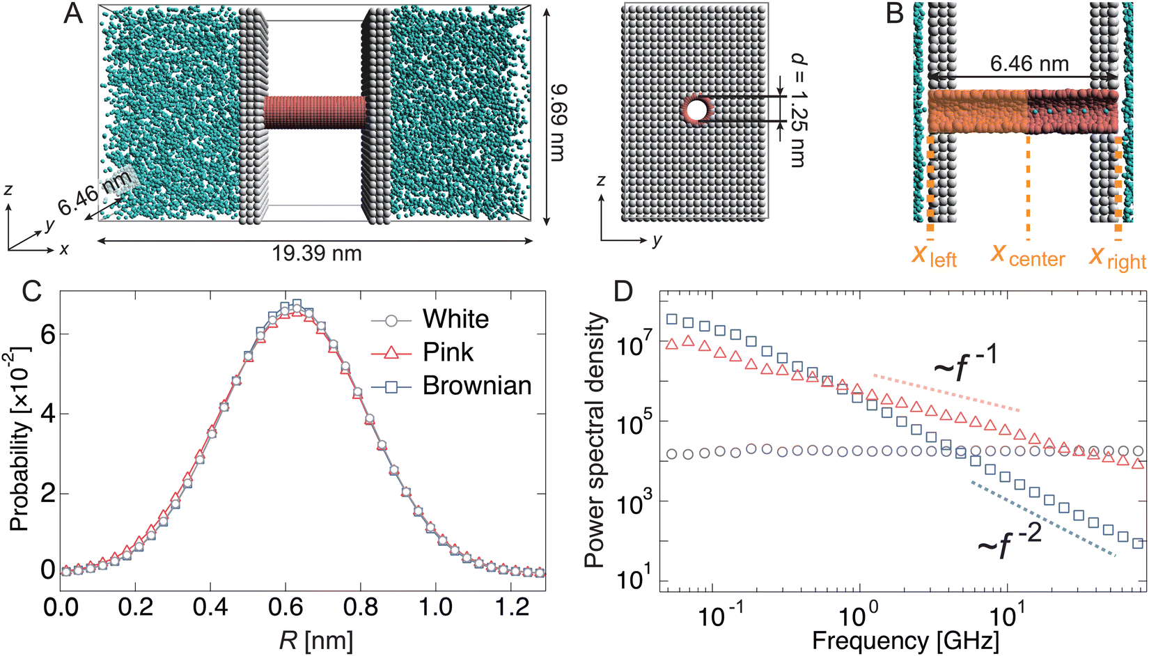Fig. 1 Active water pump model. (A) Active pump model. The water reservoirs (green) are separated by a partition (gray) that has a nanochannel (red). (B) Cross-sectional view through the center of the nanochannel. The radius of the left half of the channel (colored orange) changes its size according to certain noise. The left-end, right-end, and center positions of the nanochannel are labeled as x_left, x_right, and x_center, respectively. (C) Probability distributions and (D) power spectral density (PSD) of the radius size of the left half of the channel. The trajectory for 80 ns was used for the PSD. Gray, pink, and blue symbols represent the data obtained using white Gaussian noise, 1/f (pink) noise, and 1/f² (Brownian) noise, respectively.

Initially, the pump system was equilibrated without any radius fluctuations (passive state, see ESI,† Movie S1) for 1.0 μs, and then, the system was switched to an active (fluctuating) state for 1.8 μs to generate water flow by the active pump. Spatially asymmetric noise fluctuations imposed on the channel radius cause unidirectional water flows from the left side to the right side in the condition of no pressure difference in the reservoirs. The cumulative number (N_w) of water molecules passing from x_left to x_right was counted (Fig. 1(B) and 2(A)). When the channel radius was fluctuated according to Brownian or pink noises, a stable water flow was generated by the nanochannel (Fig. 2(A) and ESI,† Movies S2 and S3). We estimated the transport rate J, which is defined as the number of water molecules passing through the channel over 1 ns, to estimate the water transport ability. The pink noise, J, was approximately 1.0 ns⁻¹, which is the same as that of AQPs.^55,56 Interestingly, J of Brownian noise was approximately three times higher than that of pink noise. In contrast, the channel radius fluctuation given by white noise generates little water flow (ESI,† Movie S4). The energy input as a fluctuation of the channel radius performs work on the water molecules in or near the channel, and is converted into their kinetic energy. We confirmed that the temperature of the water molecules in the nanochannels is about 3 to 5 times higher than the reservoir temperature. The bounced water molecules temporarily gain kinetic energy, which is quickly dissipated because of interactions with surrounding water molecules.

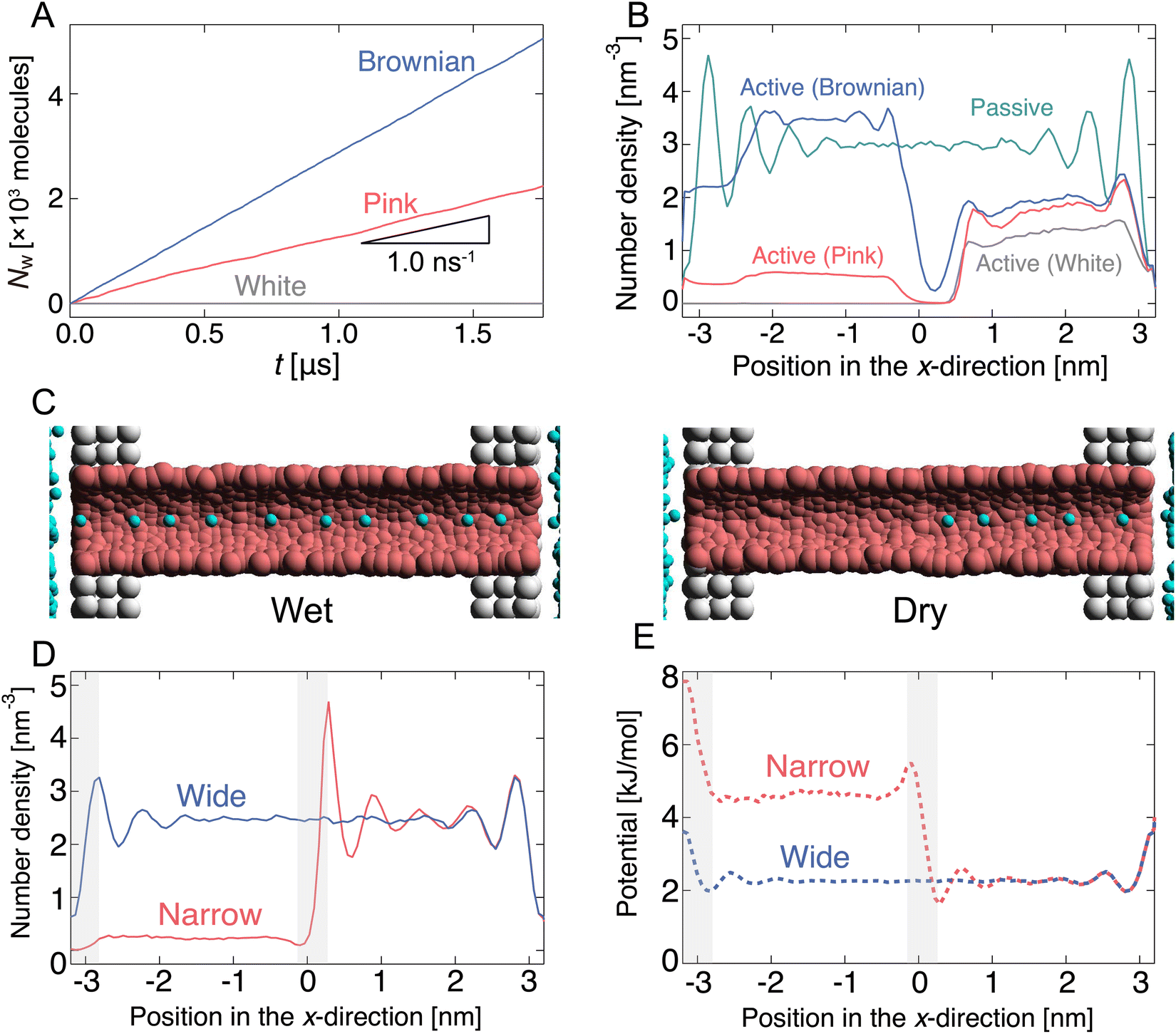Fig. 2 Water transport through an active pump. (A) Cumulative water transport through a pump driven by noise fluctuations imposed on the channel radius. (B) Number density profiles of the water molecules for passive (green) and active (gray, pink, and blue) states in the x-direction. Here, x_center is set to zero. Gray, pink, and blue colored lines represent data obtained using white, 1/f (pink), and 1/f² (Brownian) noises, respectively. Each curve is plotted based on the data averaged over 20 independent simulations. (C) Snapshots of wet and dry states in the channel. (D) Water density distribution ρ(x) along the central axis of the channel at equilibrium states. Blue and red colored curves represent ρ(x) at the wide (R = 0.623 nm) and narrow (R = 0.610 nm) radii of the channel, respectively. (E) Effective potential curves estimated by the water density distributions in the x-direction, ϕ(x) = −k_BT ln[ρ(x)/ρ₀] where ρ₀ is density in bulk.

The dependency of the flow of water on different types of noises is related to the wetting and drying conditions inside the channel. Note that wetting and drying correspond to filling and emptying in the channel with a single-file fashion of water molecules within the nanochannel. Fig. 2(B) shows the number density profiles of water molecules inside the nanochannel during the passive and active states. In the passive state, the nanochannel is filled with water molecules, and several peaks exist along the x-direction. This means that water molecules are trapped in the channel at equal intervals (Fig. 2(C)). Switching to the active state dramatically changes the density profile. At the white noise, the density of the left half (x < 0) becomes almost zero, i.e., the channel is dried at the radius fluctuating region (Fig. 2(C)). Because of the high frequency component of radius variation, water molecules cannot penetrate the channel. The densities with pink and Brownian noises are lower in most regions than those in the passive state; however, the density with Brownian noise was higher than that with pink noise overall.

Mechanism of unidirectional water transport

The direction of flow is determined by the potential change in the fluctuating area. When the nanochannel radius is sufficiently large, the water molecules are almost uniformly distributed in the channels (Fig. 2(C) and 2(D)), i.e., the potential energy is flat throughout the channel (Fig. 2(E)). In the contraction process, the potential energy in the left half of the channel increases as the channel is narrowed. We consider this phenomenon by focusing on the chemical potential (the molar Gibbs free energy G). The Gibbs free energy is defined by G = U − TS + pV. Here, U, T, S, p, and V denote the internal energy, the temperature, the entropy, the pressure, and the volume of the nanochannel. When the channel radius is large, the chemical potentials in the channel and in the reservoir are equal. As the channel radius decreases, T and p increase and V decreases. Since the time scale of the channel radius change is comparable to that of the molecular motion, the radius decreasing change of the channel is almost adiabatic and the entropy increase should be small. Therefore, one would expect the influence of U to dominate compared to the second and third terms in G. In other words, as the radius decreases, the chemical potential in the channel increases due to the increase in potential energy, and water molecules are ejected from the channel.

How then is the direction in which water is discharged from the channel determined? It is explained by the potential gradient. The water molecules located near the middle of the channel (x ∼ 0 nm) receive a rightward force because of the effect of the formation of a potential gradient. Then, the water molecules in the right half of the channel (x_center < x < x_right) are pushed to the right reservoir along the gradient with a potential difference. In contrast, it becomes difficult for water to enter and leave the channel near the left terminal (x ∼ −3 nm) because the height of the potential energy increases as the radius decreases. The potential gradient to the right formed at the left terminal also leads to flow to the right. Therefore, clearly, the potential gradient formed at the boundary between the fluctuating and the non-fluctuating regions leads to unidirectional flow through the channel.

Frequency dependence of the water flux

To investigate the dependency of the cumulative water flow on the different types of noises, we analyzed the water flow on each frequency. An additional set of simulations was performed in which the channel radius R(t) was changed with a certain frequency ω, R(t) = R₀ + A sin(ωt). Different water transports with different ω values are shown in ESI,† Movie S5, where the values of A and R₀ are the same as those in the previous simulations with different noises ξ(t). Fig. 3 shows the dependence of ω on the water transport rate J. When ω < 10⁻¹ GHz, almost no water transport occurs, i.e. J ∼ 0. In the larger frequency region, J gradually increases and reaches a maximum value (J ∼ 19.02 ns⁻¹) at ω = 7.0 GHz. After that, J rapidly decreases and becomes almost zero again at ω > 10¹ GHz. In other words, the passage of water molecules can be observed only in a certain range of frequencies (10⁻¹ < ω < 10 GHz). To demonstrate the validity of the coarse-grained MD simulations, all-atom MD simulations of similar systems were performed, as shown in Fig. S3A (ESI†). A similar dependence of the water transport rate on the frequency with a single peak was observed in the all-atom MD simulations (Fig. S3B, ESI†).

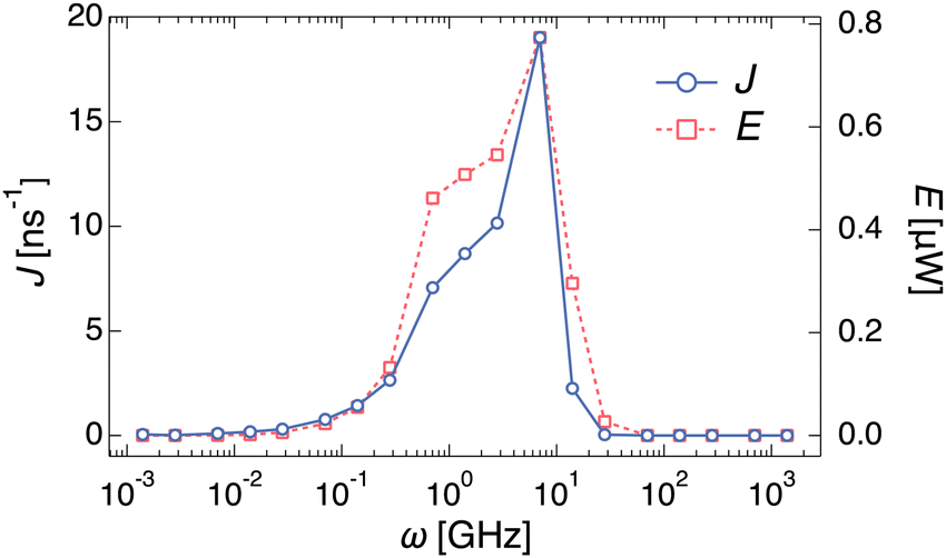Fig. 3 Frequency dependence of water molecule transport as the nanochannel radius changes according to the sine wave (R = A sin(ωt) + R₀). The left and right perpendicular axes represent the transport rate J in ns⁻¹ and the work rate E in mW, respectively.

Hysteresis in water transport by active pump

Next, we monitored the changes in N_L during the oscillation of the channel radius. Here, N_L represents the number of water molecules located in the left half of the channel. Fig. 4(A) shows the relationship between N_L and R for some representative ω values. The lower and upper arcs of the ellipse correspond to the expansion and contraction processes, respectively. The black dashed curve in Fig. 4(A) represents N_L in the equilibrium state at R, which is called the “static state.” In the static state, for R < 0.6 nm, no water can exist in the channel because the channel width is narrower than the size of the water molecules themselves. When R exceeds 0.58 nm, water begins to enter the channel.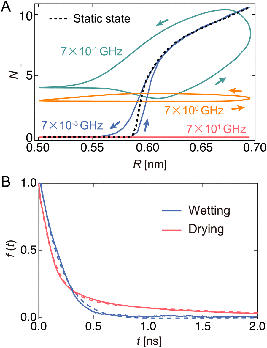

Fig. 4 Analysis of the wetting/drying dynamics in the active pump. (A) Hysteresis curves when the channel radius is controlled according to a sine wave. The perpendicular and horizontal axes represent the number of water molecules, N_L, located in the left half of the channel and the channel radius, R, respectively. The black dashed curve denotes N_L in the equilibrium state at R. (B) The relaxation curves of water molecules inside the nanochannel after instantaneous expansion (wetting) or contraction (drying) of the channel radius.

The N_L–R curves exhibit a rate-dependent hysteresis on ω. When the frequency is very low (ω = 7 × 10⁻³ GHz), a state called the “quasi-static state,” the change in N_L agrees well with the static state. The water molecules begin to penetrate the channel at the radius of R ∼ 0.6 nm in the expansion process. After that, N_L rapidly increases with increasing R, and the nanochannel is filled with ∼10 water molecules at the widest radius (R ∼ 0.7 nm). Then, it switches to a contraction process in which R gradually decreases. The water molecules are completely excreted from the channel through almost the same path as the expansion process in the hysteresis curve. At ω = 7 × 10⁻¹ GHz, the change in N_L significantly deviates from the static and quasi-static states. When R is small, a few water molecules are not discharged from the channel and remain inside the channel. Furthermore, a large hysteresis effect is observed when the expansion and contraction processes take completely different paths. As ω increases to 7.0 GHz, N_L tends to decrease overall. Thus, a flat shape is drawn in the N_L–R plane. Furthermore, hysteresis also appears in all regions of R. We call these two driving states the “pump state”. As ω increases further (ω = 7 × 10¹ GHz), no water molecules enter the channel; this state is called the “closed state”.

Origin of hysteresis and relaxation times of the wetting/drying states inside the channel

A clear hysteresis was observed during radial expansion and contraction in a certain frequency range (pump state). The hysteresis originates from the relationship between the period of expansion and contraction of the pump and the relaxation time of the wetting/drying states inside the channel. To estimate the relaxation time using this model, we monitored the temporal change in the number of water molecules N_L in the left half of the channel when R was instantly changed from the equilibrated wet (R = 0.69 nm) or dry (R = 0.57 nm) states to another state (Fig. S4, ESI†). During the drying process, N_L rapidly decreased by 0.2 ns and then started slowly decreasing, reaching almost zero at approximately 10 ns. This may correspond to two modes: one is extrusion by the nanochannel wall, and the other is escape by its own thermal diffusion. In the wetting process, water molecules rapidly fill the channel, and the steady state is reached in approximately 1.0 ns. The number of water molecules in the steady state is defined as N_C. To calculate the relaxation times of the wetting and drying processes, the time variation in f(t) is shown in Fig. 4(B). Here, f(t) is given by N_L(t)/N_L(t₀) in the drying process and [N_C − N_L(t)]/[N_C − N_L(t₀)] in the wetting process. The wetting and drying data are fitted to a single exponential curve, f(t) = A′ exp(−t/τ_wet), and double exponential curve, f(t) = A′′ exp(−t/τ_dry1) + (1 − A′′)exp(−t/τ_dry2), respectively. Thus, τ_wet, τ_dry1, and τ_dry2 are 0.348, 0.123, and 2.482 ns, respectively. Here, τ_dry1 and τ_dry2 correspond to the relaxation time forced out by tube contraction and the relaxation time spontaneously released by thermal diffusion, respectively. In this pump system, the water molecules are expelled at a faster rate than the rate with which they fill the channel (τ_dry1 < τ_wet). In the drying process, water molecules are pushed out by the pressure (p_wall) of the wall due to radial contraction, whereas in the wetting process, the reservoir is filled by the pressure (p₀) of the bulk water.

The upper and lower limits of the frequency for the hysteresis are determined by the relaxation times, τ_wet, τ_dry1, and τ_dry2. Table 1 shows half periods (P_half = π/ω), ratios of the relaxation time to P_half, transport rates J, and the corresponding pump states for the typical frequencies. We focus on the half-period here because half of a cycle is a contraction process and the other half is an expansion process. The slowest relaxation time among the three relaxation times is τ_dry2, which is the characteristic time required for water molecules to be ejected from the channel by thermal diffusion. In the quasi-static state, the period of the radial change is approximately 180 times slower than τ_dry2. In other words, water molecules are spontaneously discharged into the reservoir by diffusion without being pushed out by the channel wall. Therefore, almost no directionality exists in the outflow of water molecules, and J is extremely low (∼0.09 ns⁻¹). The fastest relaxation time, in contrast, is τ_dry1, which is the characteristic time of being pushed out of the channel by the wall surface. In the closed state, the period of radial change P_half is less than half of τ_dry1; in addition, P_half/τ_wet is only approximately 0.129. Before water can enter the channel through expansion, the channel closes by switching to the contraction process. Thus, once water is drained out, it cannot enter the channel again, and J becomes zero. In the pump state, where hysteresis is evident, the period of the change in R is in the appropriate balance between τ_wet and τ_dry1, and τ_dry2. In other words, water molecules supplied from the reservoir during the expansion process can be reliably pushed in one direction during the contraction process. Moreover, the rate of non-directional water movement due to thermal diffusion is small. The value of J at ω = 7 GHz is larger than that at ω = 70 GHz because of P_half/τ_dry2. Thus, continuous work is achieved in the pump state.

Table 1 Data list of half period P_half = π/ω, ratio of the relaxation time τ to P_half, and transport rate J for typical frequencies ω

ω [GHz]	P half [ns]	P half/τdry1	P half/τwet	P half/τdry2	J [ns^−1]	State
7 × 10^−3	449	3636	1288	181	0.09	Quasi-static
7 × 10^−1	4.49	36.4	12.9	1.81	7.06	Pump
7 × 10^0	0.449	3.64	1.29	0.181	19.02	Pump
7 × 10^1	0.0449	0.364	0.129	0.0181	0.00	Closed

---

The proposed pump system is capable of stable water transport in the frequency range of approximately 1 to 10 GHz. Zhou and Zhu³¹ performed MD simulations with a single atom of CNTs oscillating with sinusoidal waves, and showed that the kinetic energy of water molecules is strongly excited in the frequency range of 10³–10⁴ GHz. The difference in frequency order is due to the fact that they focus on the modes of hydrogen bond breaking and recombination, while we exploit the hysteresis related to drying and wetting of water molecules. Therefore, our system can achieve water transport in a lower frequency range.

Capability to overcome pressure difference

Finally, we performed simulations to investigate whether this pump system overcomes the pressure difference and can transport water. First, a separated pump system was prepared in which the reservoirs on either side of the nanochannel were unconnected and equilibrated (Fig. 5(A)). Then, after inducing R fluctuating to the channel, the density change of each reservoir (ρ_L/ρ_R) was monitored (Fig. 5(B)).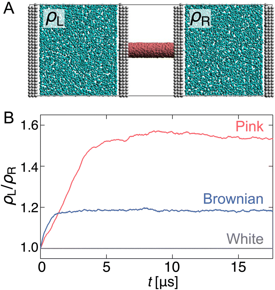

Fig. 5 Capability to overcome the pressure difference. (A) Snapshots of a separated active pump system. (B) Time series of the density difference (ρ_L/ρ_R) produced by active pumps with different noises. Here, ρ_L and ρ_R represent the number densities of the left and right reservoirs, respectively. Each curve is plotted based on the averaged data over 10 independent simulations.

As expected, when R fluctuation follows white Gaussian noise, ρ_L/ρ_R remains 1.0 because the water molecules do not pass through the nanochannel. In contrast, for pink and Brownian noises, ρ_L/ρ_R increases with time against the pressure gradient and reaches a steady state with a certain density difference. The transport rate of the Brownian noise pump is higher than that of the pink noise pump; however, it is balanced at a steady state, ρ_L/ρ_R ∼ 1.18, after t = 2 μs. The pink noise pump has a higher capability to overcome the pressure gradient, and a density difference of approximately 1.53 times is achieved in about 10 μs.

Why is it possible to achieve a higher density difference in pink noise, even though the transport rate is slower than that in Brownian noise? This can be explained by the frequency components in the pink noise. As shown in the previous section, this pump system has a characteristic relaxation time. Water transport efficiently occurs when the frequency range of the channel radius is from 7 × 10⁻¹ to 10¹ GHz, as shown in Fig. 3. As shown in Fig. 1(D), the spectral density of pink noise is higher than that of Brownian noise under most frequencies. Hence, water molecules entering from the reservoir are returned to the original reservoir by the slow radial change in Brownian noise, whereas pink noise can efficiently send them to the channel side. The thermal fluctuation of water channels such as AQPs follows 1/f noise.⁵⁰ Our results help explain the inevitability of 1/f fluctuations in biological water channels.

Similarity of the reverse Carnot cycle and energy efficiency

Additionally, the hysteresis curves (Fig. S5, ESI†) represent thermodynamic cycles, indicating that the water pump can be regarded as a nanoscale heat pump. The processes of the water pump with constant frequency roughly correspond to the following four processes of the reversed Carnot cycle; (a) adiabatic compression: contract without outflow, (b) isothermal compression: contract with outflow, (c) adiabatic expansion: expand without inflow, and (d) isothermal expansion: expand with inflow, as shown in Fig. S1 (a detailed description is written in the ESI†). The temperature in the water pump increases or decreases because of adiabatic processes caused by the radius change of the channel, which indices ejection or penetration of water molecules, respectively. The flow of water molecules induced by this process corresponds to the heat flow in a heat pump, and the water pump can behave as the nanoscale heat pump that transforms the work of radius change into molecule flow. Note that the Carnot cycle is an ideal quasi-static process and requires an infinite amount of time to execute. Therefore, the pump system proposed in this study corresponds exactly to an approximate Carnot cycle.

Using this hysteresis curve, we estimated the work rate (E) for each frequency. To estimate these as work dimensions, we converted N_L and R to p and V, respectively (Fig. S5, ESI†). In this study, p was defined as N_L multiplied by the force in the x-direction that a water molecule in the channel receives from the wall when a stable water flow is generated, and then, divided by the cross-sectional area of the channel. The volume of the left half of the channel was defined as V. E was estimated based on the area inside the p–V hysteresis curve integrated and multiplied by ω. The right axis of Fig. 3 shows the frequency dependence of E. A clear correlation between J and E was observed. As mentioned earlier, the channel radius expands and contracts in the characteristic time between τ_wet and τ_dry in this frequency region, and water flow is generated by forcing the water out through the contraction process. This workload was shown to agree well with the water transport rate.

Finally, we estimated the energy conversion efficiency (η) of the system by defining the input and output energies as the work that pushes water molecules because of the radial change and the area of the pressure–volume phase diagram (Fig. S5, ESI†), respectively. As a result, η was 0.0015 at the frequency with the highest transport rate (ω = 7 GHz). In contrast, the theoretical thermal efficiency (η_th), assuming the Carnot cycle was calculated from the temperature difference in the reservoir, and η_th was 0.0024. Note that the reservoir temperatures were calculated from simulations at a steady state. Thus, the proposed system was found to have a theoretical thermal efficiency of approximately 64%.

Future works

In this study, the interaction parameters between water molecules and nanochannels were adopted based on previous studies.^57,58 The water density distribution at the equilibrium state (as shown in Fig. 2(D)) depends on these values, thereby changing the surface energy barrier between the reservoir and the nanochannel. Arya et al.⁵⁹ applied molecular modelling techniques to zeolite systems and showed that the transport flux through nanopores is affected by these barriers. The effective potential curve (Fig. 2(E)) for the whole system is shown in Fig. S6 (ESI†). According to the results, the height of the energy barrier was about 3.78 kJ mol⁻¹ and 6.84 kJ mol⁻¹ in the wet and dry states, respectively.

The active length was also based on previous studies.^57,58 The active length represents the fraction of the nanochannel length that imposes fluctuations, therefore L_active = 50% in this simulation, as shown in Fig. 1(B). Fig. S7 (ESI†) shows the results of the L_active dependence on J for each fluctuation (white, pink, and Brownian). As expected, for white noise L_active had no effect on J, so J remained zero. For both pink and brown noise, J increased with increasing L_active when L_active > 50%. This is because many water molecules enter the channel during the expansion process and are pushed out all at once during the contraction process. However, the increase in L_active causes an increase in input energy, which may reduce the transport energy efficiency. On the other hand, the behaviour when L_active is less than 30% is interesting. In the case of pink noise, J remains above 1.0 ns⁻¹ even when L_active is around 10%, almost the same as when L_active = 50%, while in Brownian noise, J decreases rapidly and is lower than J in the pink noise. This result suggests that structural fluctuations due to 1/f can provide stable water transport even with small L_active, i.e., small input energy, which may also explain the nature of biological water channels. Thus, optimising the interaction parameter and the active length may further increase the transport rate and enable efficient water transport.

In addition, we have modelled the AQPs and determined the size of the diameter D so that the water molecules are arranged in a row inside the channel. In order to transport a large amount of water, it is possible to increase the size of D in addition to preparing multiple nanochannels. As shown in Fig. S8 (ESI†), when D was prepared in the range of 1.29 to 2.58 nm, the water molecules in the nanochannels were packed in a helical or cylindrical shape depending on the size of D. Simulations of water transport by radial fluctuations using these nanochannels showed unique behaviour, such as water transport in the opposite direction in some cases. This may be due to the effects of water clustering and interlayer slip caused by the water forming a layered structure. A more detailed analysis will be investigated in future work.

Conclusion

In summary, we have provided in silico evidence for an active water transport pump driven by noise fluctuations in pore radius. Our proposed pump is independent of the external environment and can transport water while overcoming the density and pressure gradients. The proposed pump is a nanoscale energy conversion system that corresponds to a reversed Carnot cycle, which utilizes hysteresis in the expansion and contraction processes to transport water.

A hysteresis property has already been used in practical applications as an energy conversion device. For example, a Schmitt-trigger oscillator is a device that converts electrical energy into vibrational energy. The Schmitt trigger is an electronic circuit characterized by hysteresis in the output state in response to changes in the input voltage. By setting two thresholds for the input voltage, the output voltage can be switched with the delay time with a change in the input voltage. In our proposed pump system, the input and output voltages correspond to the change in the radius of the nanochannel and the number of water molecules in the channel, respectively. Because the filling and ejection of water molecules in the channel are not synchronous with the change in the channel radius, hysteresis (delay time) exists between the expansion and contraction processes.

This energy conversion system through nanotubes, similar to a reversed Carnot cycle, is driven by a radius change of only 0.2 nm, as shown in Fig. 4(A). The size of this change was sufficiently large to be achieved by thermal fluctuations, and actual water channels such as AQPs can control the amount of water that could permeate according to this mechanism. Moreover, we revealed that the structure fluctuations are a key parameter that affects water transport through the nanochannel. For water transport, the channel radius fluctuation should not follow white noise but should rather follow 1/f^α noise. This is because certain frequencies that cause drying and wetting inside the channel are mostly contained in the 1/f^α fluctuations. This may explain why many biological channels exhibit memory-dependent dynamics, e.g., 1/f^α noise and hysteresis, in structural fluctuations.

Our work proposes a new pumping mechanism that exploits the hysteresis of the wetting and dewetting cycle. With current technology, it may be difficult to experimentally construct a pump system with the mechanism we propose. On the other hand, de novo protein designs have been actively proposed recently.^60–62 To the best of our knowledge, the design of proteins focusing on fluctuations has not yet been reported, but if, for example, photoswitching molecules can be grafted inside nanochannels or transmembrane proteins with gate structures exhibiting specific fluctuations can be designed from the amino acid sequence, water transport by the proposed mechanism will eventually be possible. Another technical implementation is to control channel wettability and pore size with time-dependent external stimuli.^38,39 Combined with these studies, we believe that the water pumping system proposed here could be an effective device for low-energy artificial purification systems and for dealing with possible water shortages in the future.

Methods

Coarse-grained molecular simulation

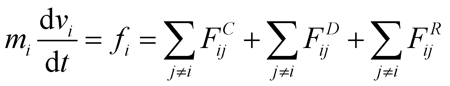
In this study, dissipative particle dynamics (DPD) simulation^63,64 was adopted to reproduce the water transportation of active pumps at the molecular level. The DPD method is a coarse-grained molecular simulation method, which has proven to be a powerful tool for investigating fluid events occurring on a wide range of spatio-temporal scales compared to all-atom simulations such as a molecular dynamics (MD) method. The coarse-grained molecular simulation method is suitable for this study because it requires more than 500 simulations on the order of μs to extract the essence of the nonequilibrium phenomenon of water transport through nanochannels. However, for some systems, the validity of the present calculations was confirmed by all-atom molecular dynamics simulations (Fig. S3, ESI†).

The DPD method is based on Newton's equation of motion, which is expressed as follows:

where i and j are the particle index, m is the particle mass, v is velocity, and f is force. Each DPD particle is subject to three types of forces (conservative (F^C), dissipative (F^R), and random (F^D)). Details of the force formula have been given elsewhere.^64,65

The results of DPD simulations are commonly reported in reduced units. The DPD unit of length is the cutoff distance (r_c), the unit of mass is the particle mass (m), and the unit of energy is (k_BT). In this study, we adopted the method developed by Groot and Rabone⁶⁵ for scaling the length and time units since the system is dominated by water behavior.

Based on our previous study,³⁴ the active water pump system comprises a nanochannel (6.46 nm < x < 12.92 nm), a water reservoir (x < 6.46 nm or x > 12.92 nm), and partition walls (x ∼ 6.46 and 12.92 nm) between the nanochannel and the reservoir. The length and diameter of the nanochannel were set to 6.46 nm and 1.25 nm, respectively. A water molecule is represented by a single DPD particle, about 3 molecules, which is commonly used in this technique. The size of this radius was optimized to fill a single row with coarse-grained water molecules, referring to a previous study.³⁴Table 2 shows the interactions between any two particles. These interaction parameters are set based on our previous motor protein systems.^57,58 The total number of particles in this model is 14 105, and the number of water and nanochannel beads is 9,083 and 1,476, respectively; the remaining particles are partitions. The volume of the simulation box is 19.39 × 6.46 × 9.69 nm³.

Table 2 Interaction parameters of pair particles a_ij (k_BT/r_c unit)

	Channel	Partition	Water
Channel	0	0	100
Partition	0	0	50
Water	100	50	25

---

By connecting the nanochannel and wall particles to their initial positions using a harmonic spring, the thermal fluctuation of the solid can be reproduced. The spring constant is set to 10⁴k_BT/r_c².³⁴ The noise parameter σ is set as 3.0, and the friction parameter γ as 4.5. The periodic boundary condition is applied in all three dimensions. All simulations are performed in the constant-volume and constant-temperature ensemble. To investigate the effect of artificial water transport through the DPD thermostat, a simulation was performed using only conservative forces to calculate the interaction with velocity scaling in a reservoir far enough away from the nanochannel. Without velocity scaling, the temperature of the system would continue to rise due to the energy of the thermal fluctuations in the nanochannel. We also controlled the momentum to zero in the direction of flow in reservoirs far enough away from the channels. The results confirm that the water transport behaviour for each noise is qualitatively consistent with the results presented in this paper.

All-atom MD simulations

We also performed MD simulations to study the behaviors of water molecules in the nanoscale active pump whose radius of the left half is changed with a certain frequency, R(t) = R₀ + A sin(ωt). The settings of the MD simulation were almost the same as those in our previous study³⁴ in which the system contains water molecules, two graphite plates, and a carbon nanotube (CNT) in a periodic boundary simulation box with size of 8.64 × 5.41 × 5.12 nm³, as shown in Fig. S3A (ESI†). The two parallel graphite plates were placed to separate the nanochannel region from the water reservoir region as well as the DPD system. The chirality and diameter of the CNT are (6,6) and 0.81 nm, respectively.⁶⁶ In the nanochannel region, the CNT is located between the graphite plates. Each plate has a hole at the place where the CNT is in contact so that the water molecules in the reservoir can flow into the CNT. The direction of the CNT is parallel to the x-axis, and the length of the CNT is 4.0 nm. The x-direction size of the reservoir is 4.64 nm, and the y and z sizes are the same as those of the simulation box. The reservoir is separately located on the left and right sides of the simulation box; however, they are connected through a periodic boundary condition. The LJ parameters σ = 0.34 nm and ε = 0.2328 kJ mol⁻¹ are used for graphite carbon atoms.⁶⁷ During the simulation, the carbon atoms are fixed.

A rigid-body model of water, the SPC/E model,⁶⁸ is employed for water molecules. The potential function of the SPC/E model includes two terms – a Coulomb term and a Lennard-Jones (LJ) term. The long-range charge–charge interactions between the water molecules can be calculated using the particle-mesh Ewald (PME) method.⁶⁹ The cut-off length of the Ewald real part and LJ interactions is 1.2 nm. Rotational motion of water molecules is calculated using the symplectic quaternion integrator.⁷⁰ The MD time step is set at 2 fs, and the total sampling simulation time is 10 ns. An MD simulation program previously developed by our group⁷¹ was employed to perform all simulations.

Water molecules were set using a simple cubic lattice in the reservoir region. The total number of water molecules was 4284. The system was equilibrated for another 1.0 ns at T = 298 K. These equilibration runs were performed in a constant-volume and constant-energy (NVE) ensemble. The sampling runs for 10 ns to estimate water flow were performed in a constant-volume and constant-temperature (NVT) ensemble with the Nosé–Poincaé method.⁷² The averaged water density in the reservoir was 1.06 g cm⁻³ in the sampling runs.

Author contributions

T. E. conceptualized the research. N. A. and T. K. conceived the research. N. A., E. Y. and K. Y. designed the analysis. N. A. and T. K. conducted the analyses. All authors discussed the results. N. A. and E. Y. mainly wrote the manuscript.

Conflicts of interest

There are no conflicts to declare.

Notes and references

1. J. R. Werber, C. O. Osuji and M. Elimelech, Nat. Rev. Mater., 2016, 1, 116018.
2. J. Shen, G. Liu, Y. Han and W. Jin, Nat. Rev. Mater., 2021, 6, 294–312.
3. M. Barboiu and A. Gilles, Acc. Chem. Res., 2013, 46, 2814–2823.
4. Y. Huo and H. Zeng, Acc. Chem. Res., 2016, 49, 922–930.
5. C. I. Lynch, S. Rao and M. S. P. Sansom, Chem. Rev., 2020, 120, 10298.
6. K. Murata, K. Mitsuoka, T. Hirai, T. Walz, P. Agre, J. B. Heymann, A. Engel and Y. Fujiyoshi, Nature, 2000, 407, 599.
7. P. Agre, L. S. King, M. Yasui, W. B. Guggino, O. P. Ottersen, Y. Fujiyoshi, A. Engel and S. Nielsen, J. Physiol., 2002, 542, 3–16.
8. B. L. de Groot and H. Grubmüller, Science, 2001, 294, 2353–2357.
9. D. F. Savage, J. D. O’Connell, L. J. W. Miercke, J. Finer-Moore and R. M. Stroud, Proc. Natl. Acad. Sci. U. S. A., 2010, 107, 17164–17169.
10. S. Gravelle, L. Joly, F. Detcheverry, C. Ybert, C. Cottin-Bizonne and L. Bocquet, Proc. Natl. Acad. Sci. U. S. A., 2013, 110, 16367–16372.
11. U. K. Eriksson, G. Fischer, R. Friemann, G. Enkavi, E. Tajkhorshid and R. Neutze, Science, 2013, 340, 1346–1349.
12. A. Horner, F. Zocher, J. Preiner, N. Ollinger, C. Siligan, S. A. Akimov and P. Pohl, Sci. Adv., 2015, 1, e1400083.
13. Y. Xiao Shen, W. Si, M. Erbakan, K. Decker, R. D. Zorzi, P. O. Saboe, Y. J. Kang, S. Majd, P. J. Butler, T. Walz, A. Aksimentiev, J. li Hou and M. Kumar, Proc. Natl. Acad. Sci. U. S. A., 2015, 112, 9810–9815.
14. E. Licsandru, I. Kocsis, Y. Xiao Shen, S. Murail, Y.-M. Legrand, A. van der Lee, D. Tsai, M. Baaden, M. Kumar and M. Barboiu, J. Am. Chem. Soc., 2016, 138, 5403–5409.
15. Y. Xiao Shen, W. Song, D. R. Barden, T. Ren, C. Lang, H. Feroz, C. B. Henderson, P. O. Saboe, D. Tsai, H. Yan, P. J. Butler, G. C. Bazan, W. A. Phillip, R. J. Hickey, P. S. Cremer, H. Vashisth and M. Kumar, Nat. Commun., 2018, 9, 2294.
16. Y. Sun and Z. Guo, Nanoscale Horiz., 2019, 4, 52–76.
17. W. Song, H. Joshi, R. Chowdhury, J. S. Najem, Y. Xiao Shen, C. Lang, C. B. Henderson, Y.-M. Tu, M. Farell, M. E. Pitz, C. D. Maranas, P. S. Cremer, R. J. Hickey, S. A. Sarles, J. li Hou, A. Aksimentiev and M. Kumar, Nat. Nanotechnol., 2020, 15, 73–79.
18. J. Shen, R. Ye, A. Romanies, A. Roy, F. Chen, C. Ren, Z. Liu and H. Zeng, J. Am. Chem. Soc., 2020, 142, 10050–10058.
19. C. J. Porter, J. R. Werber, M. Zhong, C. J. Wilson and M. Elimelech, ACS Nano, 2020, 14, 10894–10916.
20. A. Roy, J. Shen, H. Joshi, W. Song, Y.-M. Tu, R. Chowdhury, R. Ye, N. Li, C. Ren, M. Kumar, A. Aksimentiev and H. Zeng, Nat. Nanotechnol., 2021, 16, 911–917.
21. Y. Shen, F. Fei, Y. Zhong, C. Fan, J. Sun, J. Hu, B. Gong, D. M. Czajkowsky and Z. Shao, ACS Cent. Sci., 2021, 7, 2092–2098.
22. R. H. Tunuguntla, R. Y. Henley, Y.-C. Yao, T. A. Pham, M. Wanunu and A. Noy, Science, 2017, 357, 792–796.
23. Y. Li, Z. Li, F. Aydin, J. Quan, X. Chen, Y.-C. Yao, C. Zhan, Y. Chen, T. A. Pham and A. Noy, Sci. Adv., 2020, 6, eaba9966.
24. H. B. Park, J. Kamcev, L. M. Robeson, M. Elimelech and B. D. Freeman, Science, 2016, 356, eaab0530.
25. G. Hummer, J. C. Rasaiah and J. P. Noworyta, Nature, 2001, 414, 188–190.
26. S. Sriraman, I. G. Kevrekidis and G. Hummer, Phys. Rev. Lett., 2005, 95, 130603.
27. B. Corry, Energy Environ. Sci., 2011, 4, 751–759.
28. R. Garca-Fandiño and M. S. P. Sansom, Proc. Natl. Acad. Sci. U. S. A., 2012, 109, 6939–6944.
29. Winarto, D. Takaiwa, E. Yamamoto and K. Yasuoka, Nanoscale, 2015, 7, 12659–12665.
30. S. Kondrat and A. A. Kornyshev, Nanoscale Horiz., 2016, 1, 45–52.
31. X. Zhou and F. Zhu, Phys. Rev. E, 2018, 98, 032410.
32. Winarto, E. Yamamoto and K. Yasuoka, Phys. Chem. Chem. Phys., 2019, 21, 15431–15438.
33. G. Klesse, S. J. Tucker and M. S. P. Sansom, ACS Nano, 2020, 14, 10480–10491.
34. N. Arai, T. Koishi and T. Ebisuzaki, ACS Nano, 2021, 15, 2481–2489.
35. H. Lu, X. Nie, F. Wu, X. Zhou, J. Kou, Y. Xu and Y. Liu, J. Chem. Phys., 2012, 136, 174511.
36. J. Kou, X. Zhou, H. Lu, Y. Xu, F. Wu and J. Fan, Soft Matter, 2012, 8, 12111–12115.
37. X. Zhou, F. Wu, J. Kou, X. Nie, Y. Liu and H. Lu, J. Phys. Chem. B, 2013, 117, 11681–11686.
38. Z. Liu, W. Wang, R. Xie, X.-J. Ju and L.-Y. Chu, Chem. Soc. Rev., 2016, 45, 460–475.
39. Z. Zhu, D. Wang, Y. Tian and L. Jiang, J. Am. Chem. Soc., 2019, 141, 8658–8669.
40. K. F. Rinne, S. Gekle, D. J. Bonthuis and R. R. Netz, Nano Lett., 2012, 12, 1780–1783.
41. K. Xiao, Y. Zhou, X.-Y. Kong, G. Xie, P. Li, Z. Zhang, L. Wen and L. Jiang, ACS Nano, 2016, 10, 9703–9709.
42. J. Cai, W. Ma, C. Hao, M. Sun, J. Guo, L. Xu, C. Xu and H. Kuang, Chem, 2021, 7, 1802–1826.
43. Y. Li, C. Chang, Z. Zhu, L. Sun and C. Fan, J. Am. Chem. Soc., 2021, 143, 4311–4318.
44. H. Zhang, X. Hou, L. Zeng, F. Yang, L. Li, D. Yan, Y. Tian and L. Jiang, J. Am. Chem. Soc., 2013, 135, 16102–16110.
45. S. Rao, G. Klesse, P. J. Stansfeld, S. J. Tucker and M. S. P. Sansom, Proc. Natl. Acad. Sci. U. S. A., 2019, 116, 13989–13995.
46. O. Beckstein, P. C. Biggin and M. S. P. Sansom, J. Phys. Chem. B, 2001, 105, 12902–12905.
47. O. Beckstein and M. S. P. Sansom, Proc. Natl. Acad. Sci. U. S. A., 2003, 100, 7063–7068.
48. S. Kaptan, M. Assentoft, H. P. Schneider, R. A. Fenton, J. W. Deitmer, N. MacAulay and B. L. de Groot, Structure, 2015, 23, 2309–2318.
49. V. Lindahl, P. Gourdon, M. Andersson and B. Hess, Sci. Rep., 2018, 8, 2995.
50. E. Yamamoto, T. Akimoto, Y. Hirano, M. Yasui and K. Yasuoka, Phys. Rev. E: Stat., Nonlinear, Soft Matter Phys., 2014, 89, 022718.
51. R. Männikkö, S. Pandey, H. P. Larsson and F. Elinder, J. Gen. Physiol., 2005, 125, 305–326.
52. C. Tilegenova, D. M. Cortes and L. G. Cuello, Proc. Natl. Acad. Sci. U. S. A., 2017, 114, 3234–3239.
53. C. A. Villalba-Galea, Channels, 2017, 11, 140–155.
54. I. Goychuk, Phys. Rev. E: Stat., Nonlinear, Soft Matter Phys., 2009, 80, 046125.
55. M. L. Zeidel, S. V. Ambudkar, B. L. Smith and P. Agre, Biochemistry, 1992, 31, 7436–7440.
56. M. Borgnia, S. Nielsen, A. Engel and P. Agre, Annu. Rev. Biochem., 1999, 68, 425–458.
57. N. Arai, K. Yasuoka, T. Koishi and T. Ebisuzaki, ACS Nano, 2010, 4, 5905–5913.
58. N. Arai, K. Yasuoka, T. Koishi, T. Ebisuzaki and X. C. Zeng, J. Am. Chem. Soc., 2013, 135, 8616–8624.
59. G. Arya, E. J. Maginn and H.-C. Chang, J. Phys. Chem. B, 2001, 115, 2725–2735.
60. G. Bhardwaj, J. O’Connor, S. Rettie, Y. H. Huang, T. A. Ramelot, V. K. Mulligan, G. G. Alpkilic, J. Palmer, A. K. Bera, M. J. Bick, M. D. Piazza, X. Li, P. Hosseinzadeh, T. W. Craven, R. Tejero, A. Lauko, R. Choi, C. Glynn, L. Dong, R. Griffin, W. C. van Voorhis, J. Rodriguez, L. Stewart, G. T. Montelione, D. Craik and D. Baker, Cell, 2022, 185, 3520–3532.e26.
61. A. Courbet, J. Hansen, Y. Hsia, N. Bethel, Y.-J. Park, C. Xu, A. Moyer, S. E. Boyken, G. Ueda, U. Nattermann, D. Nagarajan, D. Silva, W. Sheffler, J. Quispe, A. Nord, N. King, P. Bradley, D. Veesler, J. Kollman and D. Baker, Science, 2022, 376, 383–390.
62. T. M. Chidyausiku, S. R. Mendes, J. C. Klima, M. Nadal, U. Eckhard, J. Roel-Touris, S. Houliston, T. Guevara, H. K. Haddox, A. Moyer, C. H. Arrowsmith, F. X. Gomis-Rüth, D. Baker and E. Marcos, Nat. Commun., 2022, 13, 5661.
63. P. J. Hoogerbrugge and J. M. V. A. Koelman, Europhys. Lett., 1992, 19, 155–160.
64. R. D. Groot and P. B. Warren, J. Chem. Phys., 1997, 107, 4423–4435.
65. R. D. Groot and K. L. Rabone, Biophys. J., 2001, 81, 725–736.
66. M. Oba, S. Okada and S. Maruyama, 29th Fullerene Nanotube General Symposium, 2005, Citeseer.
67. V. Bhethanabotla and W. A. Steele, Langmuir, 1987, 3, 581–587.
68. H. J. C. Berendsen, J. R. Grigera and T. P. Straatsma, J. Chem. Phys., 1987, 91, 6269–6271.
69. U. Essmann, L. Perera, M. L. Berkowitz, T. Darden, H. Lee and L. G. Pedersen, J. Chem. Phys., 1995, 103, 8577–8593.
70. T. F. Miller III, M. Eleftheriou, P. Pattnaik, A. Ndirango, D. Newns and G. J. Martyna, J. Chem. Phys., 2002, 116, 8649–8659.
71. T. Koishi and H. Takeichi, Mol. Simul., 2015, 41, 801–807.
72. S. Nosé, J. Phys. Soc. Jpn., 2001, 70, 75–77.

---

Footnote

† Electronic supplementary information (ESI) available: Similarity of the reverse Carnot cycle, validations of the simulation method and parameters, supplemental figure on hysteresis, and movie clips of water transport behaviour. See DOI: https://doi.org/10.1039/d2nh00563h

---