
 Open Access Article
 This Open Access Article is licensed under a Creative Commons Attribution-Non Commercial 3.0 Unported Licence
Multifunctional effects in magnetic nanoparticles for precision medicine: combining magnetic particle thermometry and hyperthermia
Gabriele
Barrera
 *,
Paolo
Allia
and
Paola
Tiberto
*,
Paolo
Allia
and
Paola
Tiberto
INRiM, Advanced Materials Metrology and Life Sciences, Torino, I-10135, Italy. E-mail: g.barrera@inrim.it
First published on 5th July 2023
Abstract
An effective combination of magnetic hyperthermia and thermometry is shown to be implementable by using magnetic nanoparticles which behave either as a heat sources or as temperature sensors when excited at two different frequencies. Noninteracting magnetite nanoparticles are modeled as double-well systems and their magnetization is obtained by solving rate equations. Two temperature sensitive properties derived from the cyclic magnetization and exhibiting a linear dependence on temperature are studied and compared for monodisperse and polydisperse nanoparticles. The multifunctional effects enabling the combination of magnetic hyperthermia and thermometry are shown to depend on the interplay among nanoparticle size, intrinsic magnetic properties and driving-field frequency. Magnetic hyperthermia and thermometry can be effectively combined by properly tailoring the magnetic properties of nanoparticles and the driving-field frequencies.
1 Introduction
The multifunctional properties of biocompatible magnetic nanomaterials pave the way to a variety of widespread applications in precision medicine (a.k.a. personalized medicine).1–3 In particular, magnetic nanoparticles are currently used as pointlike heat sources in magnetic hyperthermia, sensing elements in magnetic particle imaging (MPI) and/or magnetic particle spectroscopy (MPS), magnetically driveable nanocarriers for active drug targeting.4–8In magnetic hyperthermia assisted tumor therapy, the nanoparticles are excited at a sufficiently high frequency as to generate a large amount of magnetic power which is uniformly and locally transferred as heat to a diseased tissue in order either to directly destroy malignant cells9,10 or to enhance the efficacy of chemo- or radiotherapy practice by suitably increasing the temperature of the target.11–13 Therapeutic (in vivo) applications of magnetic hyperthermia have to be tailored to a patient's needs and therefore require measuring as accurately as possible the actual temperature of the target in a non-invasive way, i.e., without recurring to surgery.14,15
As a matter of fact, the multifunctional properties of magnetic nanoparticles enable them to act not only as heat sources but also as nanosensors (tracers).15,16 For instance, MPI, an ionizing radiation-free imaging technique, is currently envisaged as a mean for localizing the nanoparticles within the body, deemed to become a powerful subsidiary tool in magnetic hyperthermia therapy.17,18 Magnetic particle thermometry (MPT), i.e., the ability to measure the actual temperature of a tissue by exploiting the magnetic response of nanoparticles, can be viewed as a natural extension of the sensing properties of magnetic nanoparticles and is of no less interest in magnetic hyperthermia applications.16,19,20
Generally speaking, MPT has the obvious advantage of providing accurate information about the local temperature of a tissue without causing harm or discomfort to a patient. In principle, MPT can be implemented in a variety of ways; however, few of these can be really applied in conjunction with a typical in vivo hyperthermia treatment. It should be remarked that the experimental conditions for an efficient MPT are hardly coincident with the ones corresponding to an optimal heating performance.
In particular, magnetic hyperthermia largely arises from the magnetic losses generated by hysteresis of the particle magnetization, which should be not only maximized21–23 but also kept as constant as possible with evolving temperature in order to gain a more precise control on the whole treatment. In contrast, MPT has to be based on properties exhibiting a significant dependence on the local temperature of the host tissue. A number of more or less direct measurement techniques aimed to relate the local temperature of a host medium to the changes of some physical property have been proposed in recent years. Temperature-sensitive properties not involving the use of ionizing radiation include amplitude20,24–26 or phase16,27 of one of the higher-order harmonics of the magnetization signal, the ratio between harmonics of the same signal,19,28,29 the relaxation time of nanoparticles,30 the viscosity of the host medium,31 the proton resonance frequency or relaxation time as in MRI thermometry,32 various ultrasonic properties.14 Some techniques are applied in non-biological environments as well, as for instance in vehicle batteries33,34
Measuring the temperature via the reversible changes of the magnetic properties of the same nanoparticles used to heat a tissue (mainly through the harmonics of the picked-up signal as in MPI/MPS) is possibly the prevalent and most direct strategy,16,19,20,24–29 and one which can be equally applied to particles floating in a fluid environment or firmly blocked in a tissue. However, operating frequencies typical of MPI/MPS do not match the ones needed to obtain a good heating performance, so that making use of just one frequency26 to combine thermometry and hyperthermia may result in a non-optimal heating process. Incidentally, it should be noted that by definition a thermometric technique should never affect the temperature of the observed target, which is typically not the case when a simultaneous combination of thermometry and hyperthermia is implemented. Moreover, using a single driving frequency obviously does not allow one to measure the spontaneous cooling of a previously heated tissue.
In order to circumvent such difficulties, a possible strategy is to apply two different frequencies to the nanoparticles, making them to magnetically react in significantly different ways. Such an approach is supported by the recent development of platforms for quantitative localization of magnetic hyperthermia17,35 where two driving-field frequencies differing by more than one order of magnitude can be selectively applied on demand. In those cases the focus is more on the issues raised by the implementation of imaging than on the magnetic processes which constitute the basis of the technique, and the platforms are typically aimed at gaining information about the position of particles in the target, without attempting to implement a thermometric method.
In this work a similar two-frequency approach is proposed; however, the sensing functionality of nanoparticles driven at the lower frequency is explicitly applied to the measurement of the local temperature of a tissue rather than to imaging. The information is obtained by detection and analysis of the induced voltage generated in a pickup coil by nanoparticles submitted to the cyclic magnetization process. Two temperature-sensitive properties derived from the induced voltage are singled out and compared. It is shown that both properties are linearly dependent on temperature in the region of interest for magnetic hyperthermia therapy, so as to ensure an easy calibration of the measurement technique. Measuring the temperature can be done in the very course of a hyperthermia treatment in such a way that the therapy can be suitably guided. It is possible to get an accurate measurement of the local temperature together with a good performance of the hyperthermia treatment by suitably choosing the magnetic parameters of the nanoparticles, in accordance with the experimental conditions of the treatment. To this aim, the frequency-dependent magnetic effects occurring in magnetic nanoparticles are studied in detail.
2 Modeling the magnetization dynamics
The dynamical behaviour of non-interacting magnetite nanoparticles is described in a rate-equations framework whose advantages and limits of applicability have been clarified elsewhere.36,37 The particles are pictured as classical double-well systems (DWSs) immobilized in a host medium,37,38 so that their relaxation is dominated by the Néel's mechanism involving an activation energy barrier;39 the evolving populations of the two energy minima of the DWSs are obtained by solving the rate equations at a given temperature under a harmonic magnetic field of maximum amplitude HV and frequency f. In this way, both non-equilibrium and equilibrium configurations of the DWSs can be investigated,36,40 depending on the product of frequency and Néel's relaxation time τN: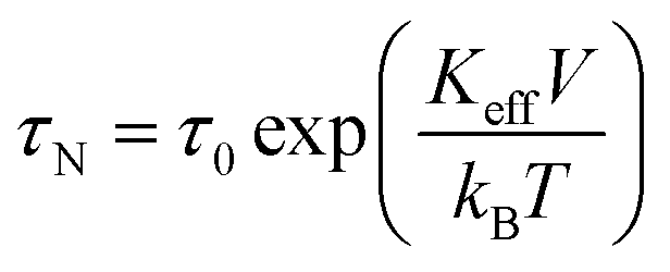 | (1) |
The DWS model applied to magnetic nanoparticles involves a specific condition on frequency to ensure detailed balance, which is achieved below f = fmax ≈ 1 × 10⁸ Hz.37 The condition τN > 1/fmax ≈ 1 × 10⁻⁸ s implies (KeffV/kBT) > 2.3 in eqn (1) in order to get reliable results by solving the rate equations. As a matter of fact, when τN is of the order of 1 × 10⁻⁸ s the population of a DWS is at equilibrium at every instant of time even in the presence of an applied field with a frequency as high as 1–2 MHz; therefore, the magnetization of the system turns out to be the equilibrium (Langevin) magnetization, which is easily evaluated without actually solving the rate equations. In addition, the condition (KeffV/kBT) > 2.3 ensures that the rate equations can be safely considered as a good approximation of the Fokker–Planck–Brown equation.37
Therefore, when (fτN) ≪ 1 and f ≲ 1–2 MHz, the solution of the rate equations for a set of nanoparticles with random easy axes naturally merges (but for a proportionality constant) with the time-dependent Langevin function:41
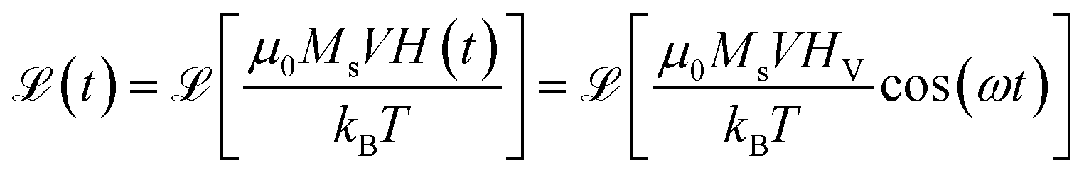 | (2) |
![[thin space (1/6-em)]](https://www.rsc.org/images/entities/char_2009.gif) cos(ωt). In this case, the outcome of the rate equation treatment is coincident with the prediction of an approximate solution to the Fokker–Planck equation derived under equivalent conditions.42 Such a simplifying assumption amounts to consider that the average alignment of nanoparticle moments always corresponds to the one dictated by the instantaneous value of the applied field, i.e., that the nanoparticle moments are able to align in times much shorter than one period of the harmonic field. Magnetic nanoparticles displaying a reversible magnetization modeled by eqn (2) are called for short ‘Langevin particles’.
cos(ωt). In this case, the outcome of the rate equation treatment is coincident with the prediction of an approximate solution to the Fokker–Planck equation derived under equivalent conditions.42 Such a simplifying assumption amounts to consider that the average alignment of nanoparticle moments always corresponds to the one dictated by the instantaneous value of the applied field, i.e., that the nanoparticle moments are able to align in times much shorter than one period of the harmonic field. Magnetic nanoparticles displaying a reversible magnetization modeled by eqn (2) are called for short ‘Langevin particles’.
In contrast, when the condition (fτN) ≪ 1 is no longer fulfilled, the cyclic magnetization process is characterized by hysteresis which naturally emerges from the rate equations.40
It should be emphasized that the DWS model, where the evolution of nanoparticle magnetization is accounted for in terms of a barrier-crossing process, cannot be directly applied to magnetic effects involving the physical rotation of the particle symmetry axes with time, a typical occurrence in particles suspended in a fluid (Brown's relaxation43). Only in the limit of vanishingly small fields, where the linear response theory can be applied,44 both Néel's and Brown's relaxation mechanisms can be treated at the same time by means of an effective time constant.43 On the other hand, in many cases of biomedical interest magnetic nanoparticles can be safely considered as immobilized in the target tissue45 because of their interaction with the cells at the cellular membrane and their subsequent internalization (process of endocytosis).46 Therefore, the rate-equation method and the Néel's relaxation framework are able to describe the effects considered in this paper despite the limitations of the DWS model.
3 MPT of monodisperse magnetic nanoparticles: a study case
In practical realizations of MPI/MPS, an optimal performance is achieved by making use of magnetite nanoparticles which exhibit a superparamagnetic (i.e., fully reversible) behaviour of the magnetization with the applied field and are able to give a sufficiently strong magnetic signal when submitted to a harmonic driving field. The operating frequency interval (10–30 kHz47,48) is basically determined by the trade-off between the need of having a high induced-voltage signal (proportional to frequency) and the one of avoiding the onset of frequency-sustained magnetic hysteresis in order not to significantly heat the nanoparticles and the surrounding tissue or material.40A way to achieve both conditions is to exploit particles made of magnetite characterized by a rather large size (typically, more than 20 nm) and by an effective magnetic anisotropy as low as 5–7 × 10³ J m−3, markedly reduced with respect to the one of bulk magnetite (approximately equal to 1–3 × 10⁴ J m−3); in this way, the energy barrier between the equilibrium positions of the DWSs is still sufficiently small to be easily overcome at room temperature and to fulfil the condition (τNf) ≪ 1 at the typical frequencies of operation.
A number of nanomaterials containing magnetite particles compatible with both requirements have been developed and made available in the last years,49 including, e.g., Resovist,50,51 a commercial, clinically approved contrast agent for magnetic resonance imaging which has been successfully applied in MPI/MPS also.52 Multi-core aggregates made of  small (≈4–5 nm) nanoparticles of magnetic moment μ(1) and effective anisotropy Keff(1) with randomly directed easy axes are an expedient solution, because the effective magnetic moment of the random aggregate is expected to increase as
 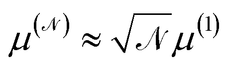 (ref. 53) and the effective magnetic anisotropy to be reduced as
 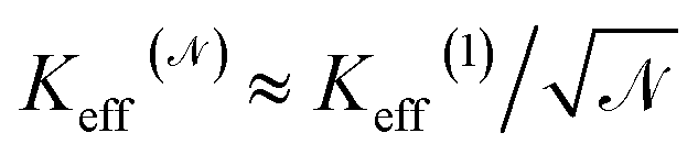 .54
.54
3.1 Effect of driving-field frequency
In the present section, we study the behaviour of non-interacting, monodisperse magnetite particles fulfilling the requirements for a good performance as sensing elements. The particles under consideration have a diameter D = 19 nm, a spontaneous magnetization Ms = 350 kA m−3 and an effective magnetic anisotropy Keff = 5 × 10³ J m−3 at room temperature. Such a value is comparable to the ones found in typical nanomaterials containing magnetite particles.49,51 It can be easily checked that they are still perfect Langevin particles at T = 300 K when submitted to a driving field of frequency f = 25 kHz (i.e., f is not sufficiently high to generate a frequency-sustained hysteresis41).However, increasing the field's frequency brings about a departure from the Langevin behaviour. The effect of frequency on the magnetization process of the particles under consideration is shown in Fig. 1, where the M(H) curves obtained from the rate equations are reported for three values of the oscillation frequency of the applied field (whose maximum amplitude HV = 7.96 × 10³ A m−1 is kept constant). As expected, when f = 25 kHz the magnetization curve is still perfectly reversible and well described by the Langevin function, whilst a hysteresis loop of width steadily increasing with increasing frequency appears for f = 250 kHz and f = 500 kHz, i.e., in the typical frequency region of magnetic hyperthermia treatments. A detail of the low-field region is shown in the upper left inset. The onset of magnetic hysteresis can be followed in the lower right inset, where the power per unit volume WL released by nanoparticles to the environment (proportional to the loop's area AL) is reported as a function of the ac field frequency (full symbols). It is interesting to compare this result to the prediction of linear response theory,44 which is easily calculated for the same parameter values through the standard formula22,44 (open symbols). In this case, the linear response theory predicts at all frequencies a much higher value of WL than actually found by the rate equation model. However, for this value of HV the linear theory can no longer be applied, as attested by the shape of the M(H) curves, which are definitely nonlinear in the considered field region. In particular, the linear response theory would incorrectly predict a nonzero value of WL even at frequencies below 50 kHz where the M(H) curve obtained by the DWS model displays no hysteresis at all (black line in Fig. 1.)
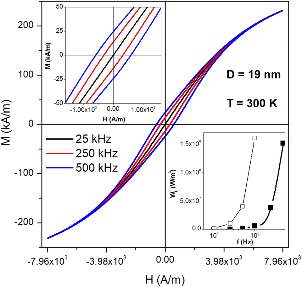 | ||
| Fig. 1 Room-temperature magnetization M of magnetite nanoparticles with D = 19 nm as a function of the driving field H for three different frequencies. Vertex field HV = 7.96 kA m−1. Inset to the left: magnification of the low-field region; inset to the right: released power per unit volume, WL, as a function of the ac field frequency (thick black line and full symbols); the prediction of the linear response theory is also reported for comparison (thin black line and open symbols). | ||
The behaviour shown in Fig. 1 for D = 19 nm as a function of frequency is related to the transition from the regime of temperature-driven (i.e., fully superparamagnetic) magnetization to the one of partially temperature-driven magnetization, corresponding to the presence of frequency-sustained hysteresis. Such a transition was defined in detail elsewhere;41 in particular, the key parameter to explain frequency-sustained hysteresis is always the product (fτN), and a simple rule of thumb can be given: fully superparamagnetic nanoparticles have to satisfy the condition (fτN) < 1/(2γ) with γ = 1–2 × 10², whilst for larger values of the product magnetic hysteresis appears by effect of the applied field's frequency.41 Taking into account eqn (1) the condition (fτN) < 1/(2γ) can be transformed into a condition for the nanoparticle diameter:
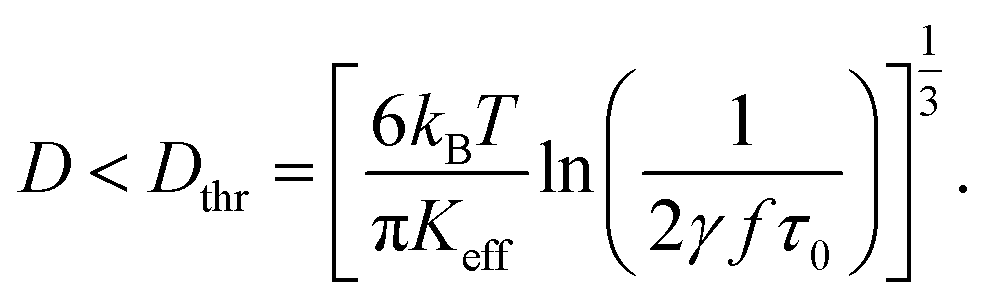 | (3) |
Showing that the threshold diameter Dthr is a function of both f and Keff at each temperature. Magnetite nanoparticles with effective anisotropy Keff behave as Langevin particles at the frequency f when their size satisfies to the inequality. In contrast, the magnetization process of particles larger than the threshold diameter is necessarily characterized by a frequency-sustained hysteresis. A graphical representation of eqn (3) is given in Fig. 2 as a colour-contour map, where the common logarithm of the applied frequency is reported on the lower x-axis.
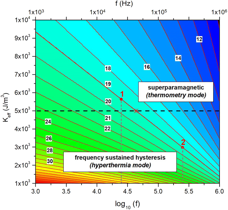 | ||
| Fig. 2 Graphical representation of eqn (3) in the frequency-magnetic anisotropy plane. Each sloping line in red is the locus of the points corresponding to the threshold diameter Dthr for a given particle diameter and any pair of values of f and Keff. Some particle diameters D (in nanometers) are indicated by the labels on the corresponding red lines. The horizontal black line represent a selected value of Keff. The intersection of the sloping line for a given D and the black line (marked by the red asterisk in the case D = 19 nm) determines the frequency f at which D is the threshold diameter Dthr. When driven at a lower frequency (case 1), particles with D = 19 nm are still superparamagnetic; when driven at a higher frequency (case 2) they display frequency-sustained hysteresis (see text for more details). | ||
The red lines in Fig. 2 are the loci of the points on the (log10(f), Keff) plane corresponding to the threshold diameter for any pair of values of frequency and effective anisotropy. These lines correspond to a set of values of the nanoparticle diameter D at intervals of one nanometer (as indicated by the black labels). For a given value of the effective anisotropy (e.g., Keff = 5 × 10³ J m−3, corresponding to the horizontal dashed black line in Fig. 2), the red lines intersect the black line at different values of the abscissa, corresponding to the frequencies where each diameter D is the threshold diameter for the selected Keff value. As an example, let us consider the particular case D = 19 nm; the intersection point between the red and the black line, indicated by the asterisk, is at log10(f) ≈ 4.64, corresponding to a frequency f ≈ 43.7 kHz. Therefore, for such a pair of coordinates Dthr ≡ 19 nm, so that by eqn (3) all particles having diameter less than 19 nm are fully superparamagnetic whilst the ones having larger diameters display frequency-sustained hysteresis when magnetically driven at 43.7 kHz.
Now, let us assume that the driving-field frequency applied to nanoparticles with D = 19 nm is equal to 25 kHz, a value currently used in MPI/MPS. In this case the abscissa takes the approximate value log10(f) ≈ 4.40; there, the threshold diameter is between 19 and 20 nm, as it can be easily checked in Fig. 2, and the representative point for D = 19 nm is above the horizontal black line (red dot designated by the label “1”), indicating a fully SP behaviour, as actually obtained by solving the rate equations (see the M(H) black line in Fig. 1). In contrast, when the operation frequency is brought to 250 kHz, a value typical of magnetic hyperthermia treatments, log10(f) ≈ 5.40; there, the threshold diameter is close to D = 16 nm, so that the representative point for D = 19 nm is well below the black line (red dot designated by the label “2”), indicating the presence of frequency-sustained hysteresis, as indeed observed in Fig. 1.
Of course, Fig. 2 can be used for any selected pair of values of Keff and frequency. It is apparent from this discussion that the onset of the frequency sustained regime of magnetic nanoparticles submitted to an ac driving field depends on three parameters: effective anisotropy, temperature, frequency, the last one being often the sole under the user's control.
The transition from irreversible to fully reversible magnetization, triggered in magnetic nanoparticles by a change of the driving field frequency, paves the way to a combination of magnetic hyperthermia and MPT. In fact, the same nanoparticles used as active heat generators for magnetic hyperthermia can be exploited as passive temperature sensors when excited at a lower frequency. A major advantage of such a multifunctional behaviour is the possibility to directly measure in real time the local temperature of a heated tissue within a living body, which is a generally difficult task, the measurement being implemented via sensors present in the tissue itself. This can allow the user to precisely control the hyperthermia session and to better tailor a specific treatment on the basis of the therapeutic prescriptions. Particles characterized by a transition from anhysteretic to hysteretic magnetization (and vice versa) in dependence of the field's frequency can be said to switch from the “hyperthermia mode” to the “thermometry mode” (and vice versa) by simply acting on the driving-field frequency, and can therefore be exploited as sensing elements in MPT.
3.2 Insight on the thermometry mode
It has been shown that magnetite nanoparticles characterized by D = 19 nm, Ms = 350 kA m−3, Keff = 5 × 10³ J m−3 are still perfect Langevin particles at room temperature and under an ac field of 25 kHz. Actually, both Ms and Keff monotonically decrease with increasing temperature,22,55,56 the reduction being stronger or weaker depending on the Curie temperature TC of the nanoparticles (the actual temperature behaviour of both properties will be better described in Section 5). Therefore, a particle which is already superparamagnetic at room temperature will remain a Langevin particle over the whole interval of temperatures spanned in a typical treatment of magnetic hyperthermia (i.e., up to about 340 K), because the energy barrier (KeffV) entering the expression of τN (see eqn (1)) is steadily reduced, so that the product (τNf) becomes increasingly smaller with increasing T.In this case it is possible to exploit the recently derived, analytical expressions for the time- and frequency-dependent properties of the Langevin function whose argument contains a harmonic driving field,57 allowing one to envisage specific methods to measure the temperature of the tissue surrounding the nanoparticles. In the following sections, two particularly promising properties are discussed and shown to provide information about the local temperature of a target containing Langevin particles in the thermometry mode.
The overall induced voltage VS (per unit area of the pickup coil's effective cross-section) is
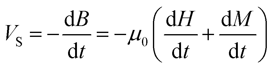
The magnetic field H(t) = HVcos(ωt) is applied to Langevin nanoparticles of volume V, so that the resulting magnetization is assumed to be 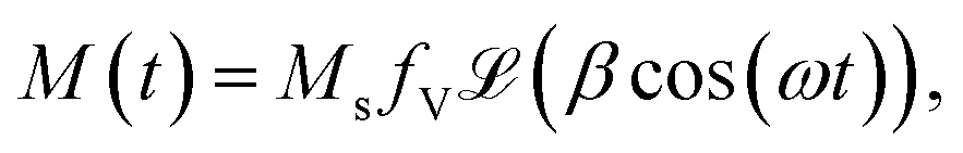 where β = μ0MsVHV/kBT is a dimensionless parameter and
  is the Langevin function. In this case, the mean square voltage (MSV) per unit area (proportional to the power dissipated in the pickup coil) is
| 〈ṼS2〉 = μ02(PH + PHM + PM) | (4) |
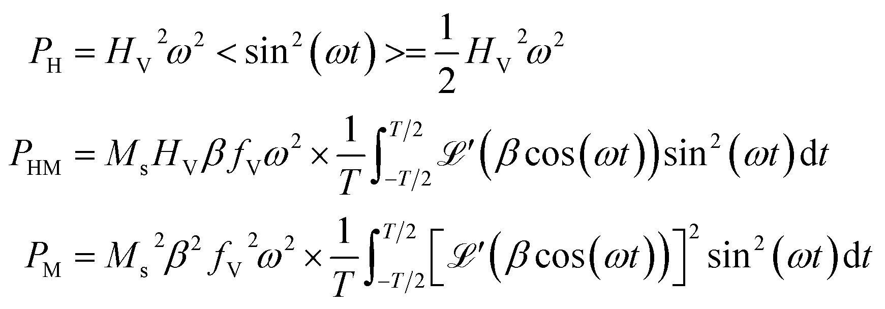 | (5) |
 is the first derivative of the Langevin function. The last two integrals in eqn (5) can be rewritten as:
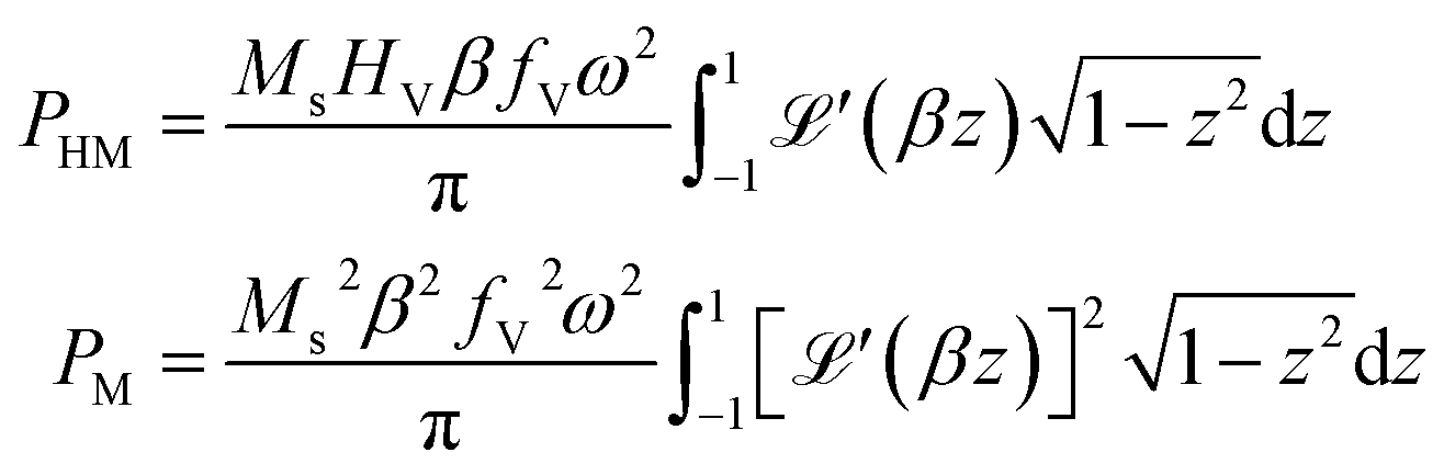 | (6) |
 so that
 | (7) |
Recalling the definition of β, it can be concluded that PHM ∝ Ms2 and PM ∝ Ms4 for T → TC.
The PH term is a known quantity, independent of both temperature and nanoparticle concentration, and can be easily subtracted, giving rise to the temperature-sensitive mean square voltage:
| 〈VS2〉 = 〈ṼS2〉 − μ02PH = μ02(PHM + PM) | (8) |
In the interval 300 K ≤ T ≤ 340 K such a quantity varies almost linearly with temperature, as shown in Fig. 3, black symbols, and can therefore be easily exploited to measure the tissue's temperature. Such a linear behaviour is a general property observed for all D and Ms values.
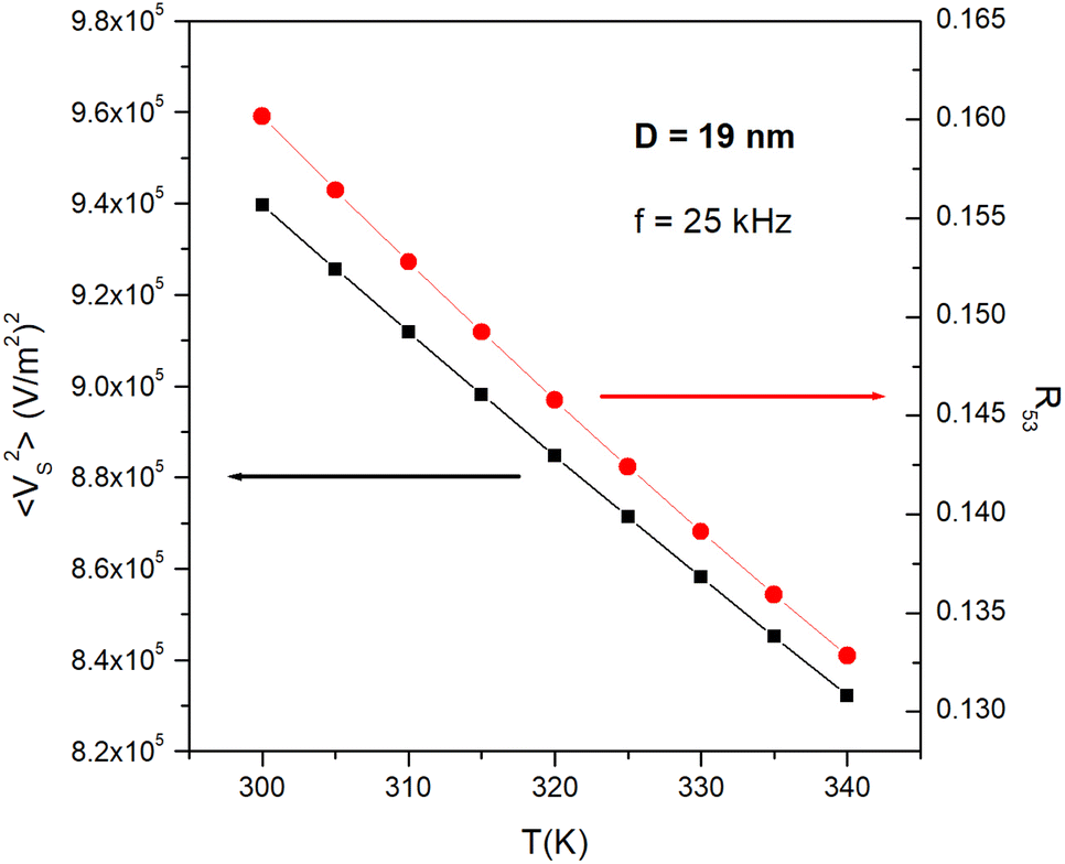 | ||
| Fig. 3 Linear behaviour of the temperature-sensitive mean square voltage (black symbols and line) and of the harmonics ratio R53 (red symbols and line) for magnetite nanoparticles with D = 19 nm in the typical temperature interval of hyperthermia therapy. | ||
cos(ωt),57 so that an expression for the ratio R53 = |V5/V3| can be easily obtained.
It should be recalled that in Langevin particles the spectral harmonics are real functions of the argument β = μ0MsVHV/kBT alternatively taking positive and negative values (for n = 1, 5, 9, … and n = 3, 7, 11, …, respectively).
The amplitude of the third harmonic of the time-dependent magnetization M(t) is:
 | (9) |
In the limit β → 0, A3 ≈ −(Ms/180)β3.
The amplitude of the fifth harmonic of M(t) is:
 | (10) |
In the limit β → 0, A5 ≈ (Ms/7560)β5.
The amplitudes of the corresponding harmonics of the induced voltage are proportional to the quantities nAn(n = 3, 5), the proportionality constant being determined by the experimental conditions.57 However, the constant is the same for all harmonics of the induced voltage, so that the R53 ratio is simply given by:
 | (11) |
In the limit β → 0, R53 ≈ β2/42.
The R53 ratio has an almost linear temperature dependence in the temperature interval 300 K ≤ T ≤ 340 K it, as shown in Fig. 3, red symbols. Such a linear behaviour is a general feature, observed for all values of D and Ms.
3.3 Prerequisites for an accurate MPT
Both MPT techniques involve magnetic nanoparticles able to switch from the hyperthermia mode to the thermometry mode by effect of a change of the driving-field frequency from a higher to a lower value. However, two conditions should be fulfilled in order to ensure an accurate temperature measurement: in the first place, the heating ability of nanoparticles should be completely turned off when they begin operating in the thermometry mode; in the second place, the change of the ac-field frequency of operation is expected to introduce a dead time; in the time interval needed to modify the frequency the tissue is no longer heated, and the local temperature begins to change. Therefore the dead time, if any, should be such as to avoid an appreciable decrease of the tissue temperature before the onset of the thermometry mode. The two issues will be separately dealt with in the following sections.In the case of Langevin particles driven at 25 kHz, the magnetic induction B(t) = μ0[H(t) + M(t)] is always in phase with the driving field H = HVcos(ωt). The space- and time-averaged electrical power (per unit volume) released by the eddy currents induced in the tissue is:58
WV = ![[small sigma, Greek, macron]](https://www.rsc.org/images/entities/i_char_e0d2.gif) μ02(HV2 + 2HVMV + MV2)f2rmax2 μ02(HV2 + 2HVMV + MV2)f2rmax2 | (12) |
is the mean electrical conductivity of the medium and MV the vertex magnetization. Using the following parameter values: = 0.025 S m−1 (appropriate, e.g., to human liver59), HV = 7.96 × 10³ A m−1, MV = fVMs with Ms = 350 kA m−1, fV = 0.01, rmax = 0.1 m, the released power per unit volume of the cylindrical piece of tissue turns out to be WV(25 kHz) = 18.8 W m−3, an exceedingly low value, certainly not enough to heat the host medium.22,60
At the frequency used in the hyperthermia mode (f = 250 kHz) the same contribution to the power per unit volume is increased by two orders of magnitude: WV(250 kHz) = 1.88 × 10³ W m−3, a value still way too low to produce a substantial increase of the temperature in the host tissue. However, a hysteresis loop is now present: the power released by the same fraction fV of hysteretic nanoparticles, which is proportional to the loop's area, turns out to be WL = 6.65 × 10⁵ W m−3 at T = 300 K, i.e., more than two orders of magnitude larger than WV(250 kHz) and more than four orders of magnitude larger than WV(25 kHz). It is precisely this contribution which acts to effectively heat the host tissue in magnetic hyperthermia.†
It is concluded that the power released by Langevin particles at f = 25 kHz is so small that the target tissue is not heated at all when the thermometry mode is turned on.
4 Effect of nanoparticle size and size distribution on MPT
Usually, ferrofluids containing magnetite nanoparticles (either single-core or multi-core) used in biomedical applications are characterized by a wide distribution of particle sizes.61–64 Therefore, it is useful to study how the size affects the magnetic behaviour at f = 25 kHz and therefore the measurement of local temperature by particles operating in the thermometry mode.4.1 Effects related to the onset of frequency-sustained hysteresis
The main size-dependent feature of magnetic nanoparticles driven at 25 kHz is the onset of frequency-sustained hysteresis above a threshold diameter (see eqn (3)). Both measurement methods proposed in Section 3.2 are based on the detection of the voltage generated by magnetic nanoparticles; as a consequence, it is helpful to discuss the effects of incipient magnetic hysteresis on the time and frequency behaviour of this property.With the parameter values used in this work, nanoparticles with D ≳ 20 nm are no longer Langevin particles at T = 300 K when they are driven at 25 kHz, and exhibit a frequency-sustained magnetic hysteresis which increases with increasing D (see Fig. 2). This can be checked in panel (a) of Fig. 4, where the M(H) curves for three particle diameters (D = 19, 21, 23 nm) with vertex field HV = 7.96 × 10³ A m−1 are shown. The curves are obtained by plotting the solutions of the rate equations M(t) as functions of H(t) and are observed to become steeper with increasing D (a larger D value brings about a larger magnetic moment); however, the dominant effect is the presence of an increasingly wider hysteresis loop when D becomes larger than 20 nm.
 | ||
| Fig. 4 (a) Effect of nanoparticle size on the shape of hysteresis loops at f = 25 kHz with HV = 7.96 kA m−1; (b) corresponding deformation of the VM(t) = dM/dt curves (one period of the field is shown); the VH = dH/dt curve is reported for comparison (dotted line); inset: region around the maximum; (c) absolute value of the ratio of n-th harmonic (Vn) to the first harmonic (V1) of the induced voltage as a function of n, for n ≤ 11 and for three particle sizes; open symbols: results of the rate equations; full symbols: theoretical prediction for Langevin particles; (d) corresponding phases ϕn obtained from the rate equations. | ||
The voltage per unit area of the pickup coil generated by the magnetization (VM(t) = −μ0dM/dt) is shown in panel (b) of Fig. 4 for the three particle diameters. In this panel, one period of the voltage generated by the applied field (VH(t) − μ0dH/dt) is reported for comparison (dashed line); an enlargement of the first half-period is shown in the inset. When D = 19 nm, VM is still perfectly in phase with VH, as expected for a Langevin particle, and results in the reversible M(H) curve shown in panel (a) (black line); in contrast, the VM(t) curve of particles displaying magnetic hysteresis is increasingly deformed and its maximum is shifted with respect to the one of the VH(t) curve.
The transition from Langevin to hysteretic particles on increasing D is observed in the frequency domain as well. The absolute values of the spectral harmonics of the induced voltage at T = 300 K for particles with D = 19, 21, 23 nm are reported in panel (c) of Fig. 4 in the form of the ratio |Vn/V1| for n ≤ 11. The results for D = 19 nm are perfectly coincident with the exact prediction for Langevin particles, as expected; in contrast, for D ≳ 20 nm the absolute values of the harmonics obtained solving the rate equations deviate from the prediction for Langevin particles of the same size, showing a much smaller reduction of the ratio |Vn/V1| with increasing n. This is a distinctive signal of the increasingly greater role played by higher-order harmonics on the M(t) curve when a hysteresis loop appears.
The phases ϕn of the harmonics for the same particle diameters are shown in panel (d) of Fig. 4. For D = 19 nm, the phases alternatively take the values (0, 180°), reflecting the change of sign of the harmonics of the time-dependent Langevin function.57 For D ≳ 20 nm, the ϕn's depart from the values expected in the Langevin case, the deviation being increasingly more pronounced as n increases.
Therefore, the onset of magnetic hysteresis has effects on the induced voltage both in the time domain and in the frequency domain, and is therefore expected to affect in some way both proposed temperature measurement methods, as shown in Fig. 5.
 | ||
| Fig. 5 (a) Effect of nanoparticle size on the temperature-sensitive mean square voltage at two different temperatures; full lines with symbols: results of rate equations; dashed lines: theoretical predictions for Langevin particles; (b) the same as in (a) for the harmonics ratio R53. | ||
The temperature-sensitive MSV is plotted in panel (a) as a function of nanoparticle diameter for 15 nm ≤ D ≤ 25 nm and for two temperatures. The explored range of diameters encompasses the transition from Langevin to hysteretic particles at the operating frequency, as easily checked in Fig. 2. The MSV is observed to display a characteristic change of slope corresponding to the change from anhysteretic to hysteretic magnetization; 〈VS2〉 increases with increasing particle diameter D; however, magnetic hysteresis brings about a reduction of the MSV with respect to the values predicted for Langevin particles (dotted lines in Fig. 5). This can be explained by recalling that an increasingly larger fraction of the energy associated with the stray induction field generated by the nanoparticles is lost to sustain the hysteresis loop.
The R53 ratio is plotted in panel (b) of Fig. 5 as a function of nanoparticle diameter in the same interval of D values and for the same two temperatures as in panel (a). As a consequence of the changes in the spectral harmonics, R53 departs from the prediction for Langevin particles above D = 20 nm, as shown in Fig. 5. The upward curvature displayed by R53 is explained considering that an increasingly larger contribution of |V5| with respect to |V3| is to be expected with increasing magnetic hysteresis, i.e., with increasing D.
Comparing panels (a) and (b) of Fig. 5, it can be deduced that the ratio R53 is less sensitive than the MSV to the onset of magnetic hysteresis.
4.2 Size distribution of particles
The effect of a size distribution on the temperature behaviour of both 〈VS2〉 and R53 is studied by assuming a Gaussian distribution of nanoparticle diameters p(D) centred at D = 20 nm and with increasing values of the standard deviation σD (2, 4, 6 nm; see panel (a) of Fig. 6).‡ The p(D) function with σD = 2 nm is similar, e.g., to the distribution of magnetic sizes experimentally observed in a batch of nanoparticles synthesized for MPI/MPS applications;63 the one with σD = 6 nm significantly deviates from monodispersity. According to our previous considerations, the p(D) function includes diameters of nanoparticles exhibiting both anhysteretic and hysteretic magnetization.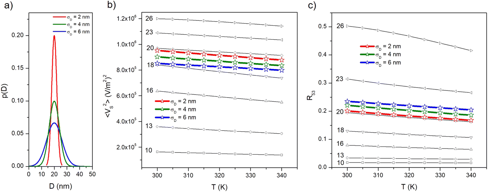 | ||
| Fig. 6 (a) Gaussian size distribution functions p(D) centred at D = 20 nm characterized by increasing values of the standard deviation σD; (b) temperature behaviour of 〈VS2〉 for nanoparticles distributed in size according to the p(D) functions (lines in colour with symbols); the corresponding curves for selected diameters are shown for comparison (black lines with symbols); (c) the same as in (b) for R53. | ||
The temperature-sensitive MSV for some selected D values is reported in panel (b) in the 300 K ≤ T ≤ 340 K along with the average curves obtained in the case of size distribution with different σD. It can be observed that the linear behaviour of 〈VS2〉(T) in the temperature interval of interest is preserved for all diameters, the main effect of magnetic hysteresis for D ≳ 20 nm being a slight change of slope of the straight lines. The average curves display a perfectly linear behaviour too, with a slightly higher slope in the case of the narrowest distribution of particle sizes.
The behaviour of the R53 ratio in the same temperature interval and for the same nanoparticle diameters is shown in panel (c) along with the average curves obtained in the case of the three size distributions. In this case, a good linear behaviour with T is observed up to D = 22 nm whereas a slight bending of the curve takes place at higher D values. However, the average curves display a perfectly linear behaviour with a slope very similar to the one of Langevin particles.
Therefore, it can be concluded that a realistic distribution of nanoparticle diameters does not appreciably modify nor worsen the functional properties which are at the basis of the proposed methods for the local temperature measurement. Of course, dealing with a size distribution implies that in a fraction of particles (the ones with larger Ds) magnetic hysteresis begins to emerge even at the lower frequency, i.e., in the thermometry mode. As a consequence, a limited heating effect could result, in contrast with the basic prescription for an ideal temperature sensor (which is naturally fulfilled by Langevin particles, see Fig. 2); however, such an undesired effect is strongly limited by the operation frequency, which is one order of magnitude lower than the ones exploited for efficient heating of a tissue by magnetic hyperthermia.
On the other hand, one can ask whether the presence of a size distribution has a negative or positive effect on the power released by the nanoparticles in the hyperthermia mode. A discussion reported in Appendix 8.2 shows that a distribution of particle diameters improves the nanoparticle performance as heat generators in the hyperthermia mode without affecting their efficiency as sensors in the thermometry mode.
5 Curie temperature and MPT
So far, the present study has been focused on nanoparticles of magnetite (Fe3O4), whose intrinsic Curie temperature TC (i.e., the temperature where the transition from ferrimagnetism to paramagnetism takes place in the particles) is around 855 K.55,65 The typical behaviour of Ms and Keff between 300 K and TC is shown in panel (a) of Fig. 7 (black lines): the curve for the spontaneous magnetization of magnetite is taken from the literature,55 the one for the magnetic anisotropy is of the type Keff ∝ Ms3,22,66 appropriate to uniaxial anisotropy.66 In the narrow interval of temperatures of interest for magnetic hyperthermia therapy (300 K ≲ T ≲ 340 K) the small reduction of both Ms and Keff concurs to enhance the negative slope of the linear variation of both 〈VS2〉 and R53 with T (see, e.g., Fig. 3). A larger effect, resulting in a higher sensitivity of MPT, could be obtained for a TC closer to the interval of temperatures of interest.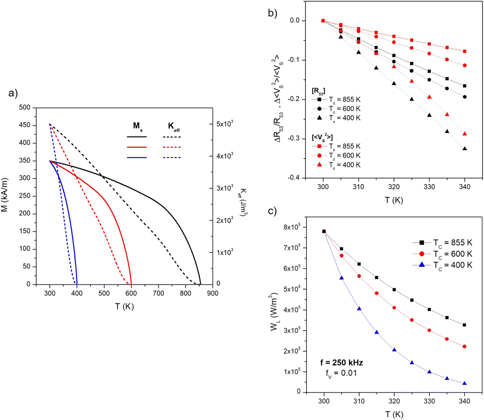 | ||
| Fig. 7 (a) Temperature behaviour of spontaneous magnetization and effective anisotropy of magnetite nanoparticles from room temperature up to the Curie temperature (full/dashed black lines, respectively); the same quantities are plotted for two materials with Curie temperatures of 600 K (full/dashed red lines) and 400 K (full/dashed blue lines); (b) relative variations with temperature of the two properties studied in this work for three Curie temperatures; (c) temperature behaviour of the power per unit volume released by nanoparticles to the environment for the same Curie temperatures. | ||
As a matter of fact, nanoparticles characterized by low Curie temperatures have been investigated in the last years in view of their possible application to self-regulating magnetic hyperthermia.67 In particular, Zn-substituted ferrites,68 quaternary ferrites such as Mg1−xFe2−2xTixO4 (ref. 69) mixtures of MgO, Fe2O3 and TiO2,70 manganite perovskites La1−xSrxMnO3,65,71 Cr3+-substituted Co–Zn ferrites72 are characterized by Curie temperatures much lower than the one of magnetite nanoparticles (i.e., mostly ranging between 330 and 380 K). These nanoparticles are studied with the aim of developing a therapy protocol based on self-regulating magnetic hyperthermia by exploiting the “on–off” characteristics of heat generation by magnetic nanoparticles below and above their intrinsic Curie temperature.65,68–72 One problem with low-TC materials is that just below the Curie temperature the spontaneous magnetization is usually very small, possibly resulting in a reduced heating effect.
In order to single out the effect of a Curie temperature lower than the one of magnetite on the performance of particles operating in the thermometry mode, we consider here ideal particles keeping the same room temperature values of Ms and TC as magnetite particles (Ms = 350 kA m−1, Keff = 5 × 10³ J m−3) but characterized by TC = 600 K and TC = 400 K (the resulting temperature behaviour of magnetic parameters is indicated by the red and blue lines in Fig. 7, panel (a), respectively).
The relative variations of both properties with respect to the values at T = 300 K (i.e., ΔR53/R53 = [R53(T) − R53(300)]/R53(300) and Δ〈VS2〉/〈VS2〉 = [〈VS2〉(T) − 〈VS2〉(300)]/〈VS2〉(300)) are shown in Fig. 7, panel (b) for the three values of TC. All curves were obtained on particles distributed in size according to the p(D) function of Fig. 6, panel (a); at 25 kHz such a distribution includes both Langevin and hysteretic particles. As expected, the negative slope of the straight lines always increases with decreasing TC; it can be noted that the ratio R53 is more sensitive than 〈VS2〉 to the measurement temperature, while the effect of decreasing TC is quite the same for the two properties. Using magnetic nanoparticles characterized by a low TC turns out to be effective in enhancing the sensitivity of the temperature measurements, because the variation of both properties in the considered temperature interval attains values as high as about 30% in absolute value. Finally, it should be noted that when the Curie temperature approaches the interval of temperatures of interest for hyperthermia (TC = 400 K) the variation of 〈VS2〉 with T is no longer linear but displays a slight downward curvature. This effect mainly arises from the steep variation of Ms close to TC, which affects the temperature-sensitive MSV more than the R53 ratio.
Of course, the enhanced measurement sensitivity of particles in the thermometry mode is counterbalanced by a strong decrease in their heating ability because of the reduction of the spontaneous magnetization when TC becomes close to the operating temperature. Such a detrimental effect is shown in panel (c) of Fig. 7 for the same size distribution of nanoparticles, now in the hyperthermia mode (f = 250 kHz); in the considered temperature interval, the power released to the unit volume of the host material WL turns out to be severely reduced for particles with TC = 400 K.
It should be noted that such an issue is common to all nanomaterials envisaged for application in self-regulating hyperthermia. A possible strategy to cope with such a drawback could be to introduce in the target a mixture of two types of nanoparticles of different chemical composition, characterized by high and low TC, the former being predominantly used for magnetic hyperthermia and the latter for high-sensitivity MPT. In fact, when the mixture is submitted to a field of frequency f = 250 kHz, the heating effect is expected to predominantly come from those particles whose TC is well above the operating temperature T, because the other particles (for which TC ≳ T) basically behave as Langevin particles even at high frequency, and therefore contribute a negligible amount of heat. In contrast, both types of nanoparticles would play a similar role when driven at a much lower frequency in the thermometry mode.
6 Comparison between the proposed techniques
Advantages and disadvantages of the two temperature-sensitive parameters investigated in the previous sections are briefly discussed in view of their prospective use in MPT.With regard to the sensitivity of a measurement, the harmonics ratio R53 should be preferred over the MSV, as stated in Section 5; in addition, the MSV is more sensitive than R53 to the transition from anhysteretic to hysteretic behaviour of the nanoparticle magnetization (Fig. 5, panel (a)); as a consequence, the sensitivity of MSV to the temperature slightly decreases with increasing nanoparticle size (Fig. 6, panel (b)).
On the other hand, in a real measurement affected by unwanted noise the MSV is expected to be more robust than the ratio between harmonics. In order to clarify this point, a white noise§ of increasingly larger power was expressly introduced in the M(t) signal and the behaviour of both R53 and 〈VS2〉 with respect to the noiseless case was investigated for magnetite nanoparticles with D = 20 nm at T = 300 K and f = 25 kHz. In particular, the quantity  was varied between 60 and 15, the former value corresponding to the ideal, noiseless case. The results are shown in Fig. 8 in the form of the relative error εr of both quantities with respect to the case SNRdB = 60. Two examples of a single period of the M(t) signal with a different white noise level are shown in the inset. It can be observed than until SNRdB is larger than about 50, the two properties behave in the same way; however, for lower values of SNRdB, the ratio of harmonics R53 exhibits a larger relative error with respect to the temperature-sensitive MSV, which turns out to be virtually unaffected by noise in the whole investigated range. As a matter of fact, in actual MPI/MPS experiments, the quantity SNR is observed to take a wide variety of values, ranging from a few units (4–5) to some hundreds (500–600),73–75 corresponding to values of SNRdB in the 6–27 range, i.e., in the left-side region of Fig. 8. It should be noted that the SNR of a signal produced by magnetic nanoparticles is markedly affected by the volume fraction fV actually present in the target;76 as a consequence, when fV is low (≲0.01) such as in some MPI/MPS applications, the temperature-sensitive MSV is expected to provide more reliable experimental results.
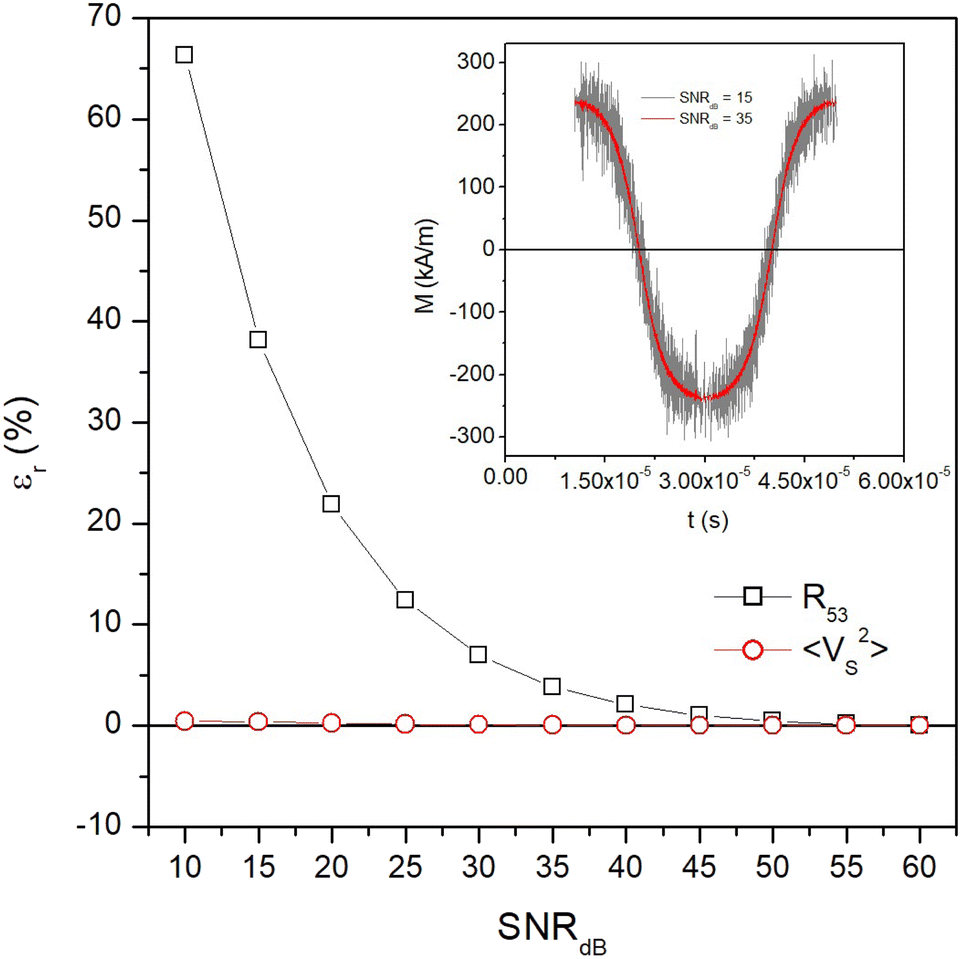 | ||
| Fig. 8 Effect of a random signal with white noise added to the M(t) signal with different values of the signal-to-noise ratio on the two studied properties for nanoparticles with D = 20 nm at T = 300 K and f = 25 kHz (examples of two noise levels are shown in the inset). The relative percent error εr with respect to the noiseless signal is reported as a function of SNRdB. | ||
7 Conclusions
The present study shows that it is possible to combine efficient magnetic hyperthermia treatments with accurate magnetic thermometry by exploiting the multifunctional properties of nanoparticles submitted to ac fields of different frequency. In this way, the thermal effect of the treatment can be suitably monitored in real time and modified on demand, thereby promoting a more efficient and accurate precision nanomedicine against cancer.The dissimilar magnetic properties of biocompatible nanoparticles driven at different frequencies allow the particles to operate either in the hyperthermia mode or in the thermometry mode. Such a dual behaviour is made possible by the frequency response of magnetic nanoparticles featuring pure Néel's relaxation. On the other hand, Brown's relaxation, neglected here, would play a role in particles still partially mobilized in the target tissue; in this case, a maximum of the magnetic losses (and therefore an unwanted heating effect) could occur at frequencies in the 10–30 kHz range also, critically depending on the Brown's relaxation time which involves the particle's hydrodynamic volume and the local viscosity of the host medium. Such an effect would be detrimental to the reliability of the thermometry mode. In line of principle, this difficulty could be circumvented by suitably tuning the maximum of the Brown's-mode contribution at a frequency different from the one used for thermometry by acting, e.g., on the particle hydrodynamic volume.
Within the Néel's relaxation framework, it is shown that the local temperature of a host tissue can be accurately measured using either of two independent temperature-sensitive properties derived from the voltage induced by the cyclic magnetization of nanoparticles.
Both the mean square induced voltage 〈VS2〉 and the ratio R53 between spectral harmonics of the magnetization are shown to exhibit a linear behaviour over the interval of temperatures involved in magnetic hyperthermia therapy so as to ensure an easy calibration of the measurement technique. The harmonics ratio turns out to be more sensitive than the MSV to temperature changes, whilst the latter property is much less influenced by signal fluctuations. These results apply to both monodisperse and polydisperse nanoparticles. Using magnetic nanoparticles characterized by low Curie temperatures enhances the sensitivity of thermometric measurements while strongly reducing the heating performance of nanoparticles in the hyperthermia mode.
In general, a good command on both hyperthermia and thermometry can only be achieved when the magnetic properties of nanoparticles are known in full detail. The multifunctional effects enabling the combination of magnetic hyperthermia and thermometry are based on the interplay among nanoparticle size, intrinsic magnetic properties and driving-field frequency. With a proper choice of all these parameters it becomes possible to measure the temperature of a tissue in the very course of a hyperthermia treatment, in such a way that the therapy can be guided according to specific needs.
8 Appendix
8.1 Cooling time of a heated tissue: a simple model
An estimate of the minimum dead time allowed during activation of the thermometry mode after turning off the hyperthermia mode is given here by requiring that spontaneous cooling down brings about a temperature decrease of no more than 0.5 K. In order to get a figure of the minimum dead time, use is made of the Fourier heat diffusion equation applied to a geometrically simple configuration characterized by realistic parameters describing the exchange of energy in living tissues.22 In particular, the heated region is assumed to be a sphere of radius b = 0.01 m made of a suitable synthetic model of a living tissue (a phantom)77 and exchanging heat with the environment through the outer surface which acts as a convective boundary.22Heat is assumed to be generated within the sphere by a uniform volume density fV = 0.01 of magnetite nanoparticles initially driven at high frequency (f = 250 kHz). Let T be the actual (absolute) temperature of the heated tissue; we define ΔT = T − Tenv the increment above the temperature of the environment Tenv (= 37 °C ≡ 310 K). It is supposed that the driving field at f = 250 kHz is switched off at time t = 0, when a parabolic temperature profile ΔT(r, 0) is present within the sphere; for t > 0 the sphere cools down. In the present configuration the evolution of ΔT for t > 0 and all r values can be obtained by solving the radial Fourier equation:
 | (13) |
where α and k are the thermal diffusivity and the thermal conductivity of the environment, the h parameter is defined as h = b|Wcb|/3, Wcb being the product between the local tissue-blood perfusion rate W and the blood's specific heat cb.79 The following parameter values, appropriate to living tissues, have been used: α = 1.4 × 10⁻⁷ m2 s−1, k = 0.5 W m−1 K−1, |Wcb| = 2000 W m−3 K−1 (for a healthy tissue) or |Wcb| = 4 × 10⁴ W m−3 K−1 (for a tissue affected by a tumor).22
The initial parabolic profile of ΔT is assumed to take a maximum and a minimum value compatible with the operating conditions of a typical hyperthermia treatment: ΔT(0, 0) = 10 K; ΔT(b, 0) = 2 K, as shown in the inset of Fig. 9. Eqn (13) is analytically solved and the resulting time evolution of ΔT at an equal distance between the sphere center and the outer surface (r = b/2) is plotted in Fig. 9 in the interval 0 ≤ t ≤ 30 s. The initial value ΔT(b/2, 0) is 8 K. The two lines refer to healthy and diseased tissues; for t ≲ 15 s hey turn out to be almost superimposed. Therefore, the dead time allowed to safely switch between hyperthermia mode and thermometry mode is more than 7 s, a condition easily fulfilled in the experimental practice, if temperature of the tissue has to be measured with a tolerance of 0.5 K.
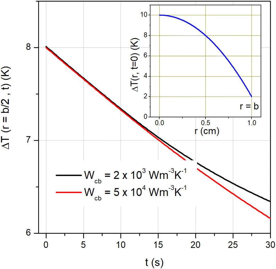 | ||
| Fig. 9 Time evolution of temperature after switching off the hyperthermia mode for two different values of the thermal parameter |Wcb|. Inset: parabolic temperature profile at t = 0 (see text for details). | ||
Although the present calculation involves a simplified heat diffusion equation79 and a very simple geometry, it nevertheless is deemed to provide the correct order of magnitude of the minimum switching time between the two modes.
8.2 Effect of particle size distribution on heat generation
Panel (a) of Fig. 10 shows the power per unit volume WL generated in the temperature interval 300 K ≤ T ≤ 340 K by a volume concentration fV = 0.01 of nanoparticles driven at f = 250 kHz and distributed in size according to the Gaussian p(D) function of Fig. 6, panel (a) (red curve and symbols). The quantity WL, which is a measure of the heating performance of nanoparticles, is related to the hysteresis loop's area AL by the relation WL = fVALf. In the same panel, the curves for selected particle diameters are also shown. The diagram of Fig. 2 predicts that at f = 250 kHz a hysteresis loop sustained by the frequency exists for D > 15 nm; in fact, particles with D = 18 nm, which display no hysteresis at f = 25 kHz, exhibit a small WL and a nonzero loop's area in the present case, as it can be checked in panel (b) where the hysteresis loops at T = 300 K for four different particle diameters are reported. | ||
| Fig. 10 (a) Temperature behaviour of the power per unit volume WL released at f = 250 kHz to the environment by nanoparticles for the distribution of sizes p(D) shown in Fig. 6, panel (a) (red line with symbols); the curves for selected diameters are shown for comparison (black lines with symbols); (b) hysteresis loops at f = 250 kHz and T = 300 K for four nanoparticle diameters (HV = 7.96 kA m−1). | ||
The power released by particles distributed in size turns out to be higher than the one corresponding to the mean diameter of the distribution (〈D〉 = 20 nm) because of the effect of the strong contributions from large particles. Therefore, a distribution of non-interacting nanoparticles with mean diameter 〈D〉 = 20 nm ensures a better heating performance than an identical volume fraction of monodisperse nanoparticles all characterized by the same diameter (D = 20 nm).
Author contributions
Gabriele Barrera: conceptualization, data curation, investigation, measurements, writing. Paolo Allia: conceptualization, data curation, formal analysis, methodology, validation, writing & editing. Paola Tiberto: conceptualization, methodology, supervision, validation, writing & editing.Conflicts of interest
There are no conflicts to declare.Acknowledgements
This work was supported by Project 18HLT06 RaCHy, which has received funding from the European Metrology Programme for Innovation and Research (EMPIR), co-financed by the participating states, and from the European Union's Horizon 2020 Programme.Notes and references
- Y. Zhang, H. Yang, Y. Yu and Y. Zhang, Theranostics, 2022, 12, 2674–2686 CrossRef CAS PubMed.
- K. S. Sunderland, M. Yang and C. Mao, Angew. Chem., Int. Ed., 2017, 56, 1964–1992 CrossRef CAS PubMed.
- F. Soto, J. Wang, R. Ahmed and U. Demirci, Adv. Sci., 2020, 7, 1–34 Search PubMed.
- E. M. Materón, C. M. Miyazaki, O. Carr, N. Joshi, P. H. Picciani, C. J. Dalmaschio, F. Davis and F. M. Shimizu, Applied Surface Science Advances, 2021, 6, 100163 CrossRef.
- M. Hepel, Magnetochemistry, 2020, 6, 1–17 CrossRef.
- X. Li, W. Li, M. Wang and Z. Liao, J. Controlled Release, 2021, 335, 437–448 CrossRef CAS PubMed.
- K. Wu, J. Liu, V. K. Chugh, S. Liang, R. Saha, V. D. Krishna, M. C. Cheeran and J. P. Wang, Nano Futures, 2022, 6, 022001 CrossRef PubMed.
- S. Balasubramanian and A. J. Cowin, in Bionanotechnology in Cancer, Jenny Stanford Publishing, New York, 2022, p. 36 Search PubMed.
- L. Beola, L. Asín, C. Roma-Rodrigues, Y. Fernandez-Afonso, R. M. Fratila, D. Serantes, S. Ruta, R. W. Chantrell, A. R. Fernandes, P. V. Baptista, J. M. de la Fuente, V. Grazu and L. Gutierrez, ACS Appl. Mater. Interfaces, 2020, 12, 43474–43487 CrossRef CAS PubMed.
- S. Piehler, L. Wucherpfennig, F. L. Tansi, A. Berndt, R. Quaas, U. Teichgraeber and I. Hilger, Nanomedicine, 2020, 28, 102183 CrossRef CAS PubMed.
- N. Pazouki, S. Irani, N. Olov, S. M. Atyabi and S. Bagheri-Khoulenjani, Prog. Biomater., 2022, 11, 43–54 CrossRef CAS PubMed.
- H. Lin, L. Yin, B. Chen and Y. Ji, Colloids Surf., B, 2022, 219, 112814 CrossRef CAS PubMed.
- N. Kulkarni-Dwivedi, P. R. Patel, B. V. Shravage, R. U. Umrani, K. M. Paknikar and S. H. Jadhav, Nanomedicine, 2023, 17, 25 Search PubMed.
- H. F. Rodrigues, G. Capistrano and A. F. Bakuzis, Int. J. Hyperthermia, 2020, 37, 76–99 CrossRef CAS PubMed.
- S. Healy, A. F. Bakuzis, P. W. Goodwill, A. Attaluri, J. W. Bulte and R. Ivkov, Wiley Interdiscip. Rev.: Nanomed. Nanobiotechnol., 2022, 14, 1–20 Search PubMed.
- E. Garaio, J. M. Collantes, J. A. Garcia, F. Plazaola and O. Sandre, Appl. Phys. Lett., 2015, 107, 123103 CrossRef.
- D. Hensley, Z. W. Tay, R. Dhavalikar, B. Zheng, P. Goodwill, C. Rinaldi and S. Conolly, Phys. Med. Biol., 2017, 62, 3483–3500 CrossRef PubMed.
- S. Harvell-Smith, L. D. Tunga and N. T. K. Thanh, Nanoscale, 2021, 14, 3658–3697 RSC.
- J. B. Weaver, A. M. Rauwerdink and E. W. Hansen, Med. Phys., 2009, 36, 1822–1829 CrossRef CAS PubMed.
- J. Salamon, J. Dieckhoff, M. G. Kaul, C. Jung, G. Adam, M. Möddel, T. Knopp, S. Draack, F. Ludwig and H. Ittrich, Sci. Rep., 2020, 10, 1–11 CrossRef PubMed.
- I. Rodrigo, I. Castellanos-Rubio, E. Garaio, O. K. Arriortua, M. Insausti, I. Orue, J. Á. García and F. Plazaola, Int. J. Hyperthermia, 2020, 37, 976–991 CrossRef CAS PubMed.
- G. Barrera, P. Allia and P. Tiberto, Nanoscale, 2020, 12, 6360–6377 RSC.
- K. Enpuku and T. Yoshida, AIP Adv., 2021, 11, 125123 CrossRef.
- C. Stehning, B. Gleich and J. Rahmer, Int. J. Magn. Part. Imaging, 2016, 2, 1–6 Search PubMed.
- J. Zhong, M. Schilling and F. Ludwig, Meas. Sci. Technol., 2018, 29, 115903 CrossRef.
- J. Wells, S. Twamley, A. Sekar, A. Ludwig, H. Paysen, O. Kosch and F. Wiekhorst, Nanoscale, 2020, 12, 18342–18355 RSC.
- J. Liu, Z. Zhang, Q. Xie and W. Liu, J. Appl. Phys., 2022, 131, 173901 CrossRef CAS.
- A. L. Elrefai, T. Yoshida and K. Enpuku, J. Magn. Magn. Mater., 2019, 491, 165480 CrossRef CAS.
- J. Zhong, M. Schilling and F. Ludwig, Phys. Rev. Appl., 2021, 16, 054005 CrossRef CAS.
- I. M. Perreard, D. B. Reeves, X. Zhang, E. Kuehlert, E. R. Forauer and J. B. Weaver, Phys. Med. Biol., 2014, 59, 1109–1119 CrossRef CAS PubMed.
- M. Utkur and E. U. Saritas, Med. Phys., 2022, 49, 2590–2601 CrossRef PubMed.
- P. Saccomandi, E. Schena and S. Silvestri, Int. J. Hyperthermia, 2013, 29, 609–619 CrossRef PubMed.
- X. Liu, W. Chen, J. Liu, W. Li and R. Yan, 2018 IEEE International Instrumentation and Measurement Technology Conference (I2MTC), 2018 Search PubMed.
- D. Zou, M. Li, D. Wang, N. Li, R. Su, P. Zhang, Y. Gan and J. Cheng, IEEE Access, 2020, 8, 135491–135498 Search PubMed.
- Z. W. Tay, P. Chandrasekharan, A. Chiu-Lam, D. W. Hensley, R. Dhavalikar, X. Y. Zhou, E. Y. Yu, P. W. Goodwill, B. Zheng, C. Rinaldi and S. M. Conolly, ACS Nano, 2018, 12, 3699–3713 CrossRef CAS PubMed.
- P. Allia, G. Barrera and P. Tiberto, Phys. Rev. B, 2018, 98, 134423 CrossRef CAS.
- P. Allia, G. Barrera and P. Tiberto, Phys. Rev. Appl., 2019, 12, 034041 CrossRef CAS.
- D. Soukup, S. Moise, E. Céspedes, J. Dobson and N. D. Telling, ACS Nano, 2015, 9, 231–240 CrossRef CAS PubMed.
- W. T. Coffey and Y. P. Kalmykov, J. Appl. Phys., 2012, 112, 121301 CrossRef.
- P. Allia, G. Barrera and P. Tiberto, J. Magn. Magn. Mater., 2020, 496, 165927 CrossRef CAS.
- G. Barrera, P. Allia and P. Tiberto, Nanoscale, 2021, 13, 4103–4121 RSC.
- D. B. Reeves and J. B. Weaver, Crit. Rev. Biomed. Eng., 2014, 42, 85–93 CrossRef PubMed.
- G. Glöckl, R. Hergt, M. Zeisberger, S. Dutz, S. Nagel and W. Weitschies, J. Phys.: Condens. Matter, 2006, 18, S2935–S2949 CrossRef.
- R. Rosensweig, J. Magn. Magn. Mater., 2002, 252, 370–374 CrossRef CAS.
- U. M. Engelmann, J. Seifert, B. Mues, S. Roitsch, C. Ménager, A. M. Schmidt and I. Slabu, J. Magn. Magn. Mater., 2019, 471, 486–494 CrossRef CAS.
- N. Oh and J.-H. Park, Int. J. Nanomed., 2014, 9, 51–63 Search PubMed.
- C. Billings, M. Langley, G. Warrington, F. Mashali and J. A. Johnson, Int. J. Mol. Sci., 2021, 22, 7651 CrossRef CAS PubMed.
- X. Yang, G. Shao, Y. Zhang, W. Wang, Y. Qi, S. Han and H. Li, Front. Physiol., 2022, 13, 898426 CrossRef PubMed.
- A. L. Elrefai, T. Yoshida and K. Enpuku, J. Magn. Magn. Mater., 2019, 474, 522–527 CrossRef CAS.
- P. Reimer, G. Schuierer, T. Balzer and P. E. Peters, Magn. Reson. Med., 1995, 34, 694–697 CrossRef CAS PubMed.
- N. Löwa, P. Knappe, F. Wiekhorst, D. Eberbeck, A. F. Thunemann and L. Trahms, IEEE Trans. Magn., 2015, 51, 4–7 Search PubMed.
- J. Haegele, N. Panagiotopoulos, S. Cremers, J. Rahmer, J. Franke, R. L. Duschka, S. Vaalma, M. Heidenreich, J. Borgert, P. Borm, J. Barkhausen and F. M. Vogt, IEEE Trans. Med. Imaging, 2016, 35, 2312–2318 Search PubMed.
- V. Schaller, G. Wahnström, A. Sanz-Velasco, S. Gustafsson, E. Olsson, P. Enoksson and C. Johansson, Phys. Rev. B: Condens. Matter Mater. Phys., 2009, 80, 092406 CrossRef.
- G. Herzer, V. Gmbh, D. Hanau and F. R. Germany, IEEE Trans. Magn., 1990, 26, 1397–1402 CrossRef CAS.
- D. J. Dunlop and O. Ozdemir, Rock Magnetism, Cambridge University Press, Cambridg, UK, 1997 Search PubMed.
- V. Aquino, L. Figueiredo, J. Coaquira, M. Sousa and A. Bakuzis, J. Magn. Magn. Mater., 2020, 498, 166170 CrossRef CAS.
- G. Barrera, P. Allia and P. Tiberto, Phys. Rev. Appl., 2022, 18, 024077 CrossRef CAS.
- W. Atkinson, I. Brezovich and D. P. Chakraborty, IEEE Trans. Biomed. Eng., 1984, BME-31, 70–75 Search PubMed.
- M. J. Peters, J. G. Stinstra and I. Leveles, in Modeling and Imaging of Bioelectrical Activity, ed. B. He, Springer, Boston, 2004, pp. 281–319 Search PubMed.
- S. Dutz and R. Hergt, Int. J. Hyperthermia, 2013, 29, 790–800 CrossRef PubMed.
- F. Ludwig, T. Wawrzik, T. Yoshida, N. Gehrke, A. Briel, D. Eberbeck and M. Schilling, IEEE Trans. Magn., 2012, 48, 3780–3783 Search PubMed.
- D. Eberbeck, F. Wiekhorst, S. Wagner and L. Trahms, Appl. Phys. Lett., 2011, 98, 182502 CrossRef.
- F. Ludwig, H. Remmer, C. Kuhlmann, T. Wawrzik, H. Arami, R. M. Ferguson and K. M. Krishnan, J. Magn. Magn. Mater., 2014, 360, 169–173 CrossRef CAS PubMed.
- A. L. Elrefai, T. Sasayama, T. Yoshida and K. Enpuku, AIP Adv., 2018, 8, 056803 CrossRef.
- M. Soleymani, M. Edrissi and A. M. Alizadeh, J. Mater. Chem. B, 2017, 5, 4705–4712 RSC.
- B. D. Cullity and C. D. Graham, Introduction to Magnetic Materials, 2009 Search PubMed.
- N. T. K. T. Thanh, Magnetic Nanoparticles From Fabrication to Clinical Applications, CRC Press, 2012, vol. 54, pp. 243–276 Search PubMed.
- A. Hanini, L. Lartigue, J. Gavard, K. Kacem, C. Wilhelm, F. Gazeau, F. Chau and S. Ammar, J. Magn. Magn. Mater., 2016, 416, 315–320 CrossRef CAS.
- G. Ferk, M. Drofenik, D. Lisjak, A. Hamler, Z. Jagličić and D. Makovec, J. Magn. Magn. Mater., 2014, 350, 124–128 CrossRef CAS.
- M. Gerosa, M. Dal Grande, A. Busato, F. Vurro, B. Cisterna, E. Forlin, F. Gherlinzoni, G. Morana, M. Gottardi, P. Matteazzi, A. Speghini and P. Marzola, Nanotheranostics, 2021, 5, 333–347 CrossRef PubMed.
- E. Natividad, M. Castro, G. Goglio, I. Andreu, R. Epherre, E. Duguet and A. Mediano, Nanoscale, 2012, 4, 3954–3962 RSC.
- W. Zhang, X. Zuo, Y. Niu, C. Wu, S. Wang, S. Guan and S. R. P. Silva, Nanoscale, 2017, 9, 13929–13937 RSC.
- M. Graeser, A. Von Gladiss, M. Weber and T. Buzug, Phys. Med. Biol., 2017, 62, 3378–3391 CrossRef CAS PubMed.
- S. Vaalma, J. Rahmer, N. Panagiotopoulos, R. L. Duschka, J. Borgert, J. Barkhausen, F. M. Vogt and J. Haegele, PLoS One, 2017, 12, 1–22 CrossRef PubMed.
- O. Kosch, H. Paysen, J. Wells, F. Ptach, J. Franke, L. Wöckel, S. Dutz and F. Wiekhorst, J. Magn. Magn. Mater., 2019, 471, 444–449 CrossRef CAS.
- S. Horvat, P. Vogel, T. Kampf, A. Brandl, A. Alshamsan, H. A. Alhadlaq, M. Ahamed, K. Albrecht, V. C. Behr, A. Beilhack and J. Groll, ChemNanoMat, 2020, 6, 755–758 CrossRef CAS.
- Y. Yuan, C. Wyatt, P. MacCarini, P. Stauffer, O. Craciunescu, J. MacFall, M. Dewhirst and S. K. Das, Phys. Med. Biol., 2012, 57, 2021–2037 CrossRef PubMed.
- D. W. Hahn and M. N. Özisik, Heat Conduction, John Wiley & Sons, New Jersey, 3rd edn, 2012 Search PubMed.
- H. W. Huang and T. L. Horng, in Heat Transfer and Fluid Flow in Biological Processes, Elsevier Inc., 2015, ch. 1, pp. 1–42 Search PubMed.
Footnotes |
| † It should be recalled that both amplitude and frequency of the driving field taken in this paper for the hyperthermia mode are such that the product (HVf) ≈ 2 × 10⁹ A m−1 s−1 is fully compatible with the Dutz–Hergt limits (Dutz 2013) for a coil of diameter comparable to rmax. |
| ‡ It should be explicitly note that p(D) is intended as the actual distribution of the magnetic cores of nanoparticles, not the one of the hydrodynamic diameters. |
| § This is assumed to be the dominant noise contribution from the measuring setup (pre-amplifiers and power amplifiers) in the frequency range 10 kHz to 1 MHz; in the same range the phase noise of typical signal generators can be assumed to be almost constant with frequency; the noise arising from external disturbances can in principle be reduced by suitably shielding the setup coils. |
| This journal is © The Royal Society of Chemistry 2023 |