
 Open Access Article
 This Open Access Article is licensed under a
 Creative Commons Attribution 3.0 Unported Licence
Real-time continuous monitoring of dynamic concentration profiles studied with biosensing by particle motion†
Max H.
Bergkamp
 ac,
Sebastian
Cajigas
d,
Leo J.
van IJzendoorn
bc and
Menno W. J.
Prins
*abcd
ac,
Sebastian
Cajigas
d,
Leo J.
van IJzendoorn
bc and
Menno W. J.
Prins
*abcd
aDepartment of Biomedical Engineering, Eindhoven University of Technology, 5612 AE Eindhoven, The Netherlands. E-mail: m.w.j.prins@tue.nl
bDepartment of Applied Physics and Science Education, Eindhoven University of Technology, 5612 AE Eindhoven, The Netherlands
cInstitute for Complex Molecular Systems (ICMS), Eindhoven University of Technology, 5612 AE Eindhoven, The Netherlands
dHelia Biomonitoring, 5612 AR Eindhoven, The Netherlands
First published on 29th September 2023
Abstract
Real-time monitoring-and-control of biological systems requires lab-on-a-chip sensors that are able to accurately measure concentration–time profiles with a well-defined time delay and accuracy using only small amounts of sampled fluid. Here, we study real-time continuous monitoring of dynamic concentration profiles in a microfluidic measurement chamber. Step functions and sinusoidal oscillations of concentrations were generated using two pumps and a herringbone mixer. Concentrations in the bulk of the measurement chamber were quantified using a solution with a dye and light absorbance measurements. Concentrations near the surface were measured using a reversible cortisol sensor based on particle motion. The experiments show how the total time delay of the real-time sensor has contributions from advection, diffusion, reaction kinetics at the surface and signal processing. The total time delay of the studied real-time cortisol sensor was ∼90 seconds for measuring 63% of the concentration change. Monitoring of sinusoidal cortisol concentration–time profiles showed that the sensor has a low-pass frequency response with a cutoff frequency of ∼4 mHz and a lag time of ∼60 seconds. The described experimental methodology paves the way for the development of monitoring-and-control in lab-on-a-chip systems and for further engineering of the analytical characteristics of real-time continuous biosensors.
1. Introduction
Real-time biosensors that enable continuous measurements of concentration–time profiles have great potential for studying the dynamics of biological and biotechnological processes and for the development of strategies to control biological systems based on measurements in real time. Here, real-time sensing refers to sensing methods that operate with time delays that are short with respect to the timescales of typical concentration fluctuations in the system of interest, allowing one to collect detailed information and to act quickly if and when needed.1 Such sensors enable closed-loop therapy control in healthcare2,3 and real-time process control in industrial applications.4–6 For example, real-time continuous glucose sensors, based on enzymatic electrochemical sensing principles, have already been established as a valuable technology for glucose control in patients with diabetes.7–9 However, enzymatic sensing is limited to reactive analytes at high concentrations.10,11 In contrast, affinity-based sensing can be applied for a wider range of analytes and a wider range of concentrations (micromolar, nanomolar, picomolar) for measuring analytes such as hormones, proteins, drugs and nucleic acids. Furthermore, the intrinsic reversibility of affinity-based interactions can be used to design sensors that are fully reversible.12,13 Examples of affinity-based sensors that have been demonstrated for real-time continuous biosensing are electrochemical aptamer-based sensors,14–16 fluorescence-based sensors17–19 and biosensors based on particle motion.20–25 These approaches have shown continuous sensing over multiple hours with time delays on timescales of minutes.The total time delay of a real-time affinity-based sensor has contributions from transport processes (advection, diffusion),26 affinity reactions,26 and signal processing.27 It is important to understand the origins of the different contributions in order to be able to design sensors that meet the needs of different applications. Lubken et al. performed simulations to study the response of a continuous affinity-based sensor depending on parameters such as the dimensions of the measurement chamber, the concentration of the analyte, and the affinity constants of the binder molecules.13 The results show that transport and reaction properties cause continuous sensors to act as low-pass frequency filters, where slow changes in concentration (low frequencies) can be measured more easily than fast changes in concentration (high frequencies).13,28 In addition, the output signals of real-time sensors are delayed by signal processing contributions,27 including the data sampling time and the time needed to analyze the measurement data.
In this paper, we present experiments that quantify the total time delay and the frequency response of a real-time cortisol biosensor based on biosensing by particle motion (BPM). Concentration–time profiles are generated using two pumps and a herringbone mixer chip29 and the sample stream is measured in the biosensing chip. We show how experiments with concentration steps can be used to extract time delays related to physicochemical processes. The transport into the measurement chamber is characterized with light absorbance measurements. Transport and reaction properties are studied using a reversible cortisol BPM sensor integrated in the measurement chamber. Sinusoidal cortisol concentration–time profiles are applied to study how the response of the sensor depends on the modulation frequency of concentration changes. Finally, we discuss how the experimental methodology can help engineers in the development of real-time affinity-based biosensors for a variety of applications.
2. Experimental section
2.1 Real-time continuous monitoring of dynamic concentration profiles
Fig. 1a outlines the questions that are addressed in this paper. The main aim is to study the total time delay of a real time sensor ΔtRTS, i.e., the time between the moment that a probed system of interest is in a certain concentration condition and the subsequent moment that the biosensor reports the corresponding concentration value. The total time delay has contributions from physicochemical processes, such as transport (advection, diffusion) and molecular reaction processes (binding kinetics), and from signal processing, including the data sampling time and the time needed to analyze the measurement data. Experiments with concentration step functions are performed to quantify the transport time delay Δt0 and the characteristic equilibration time τC. Real-time continuous monitoring of dynamic concentration profiles is studied with sinusoidal concentration profiles, which allows quantifications of the measured concentration change ΔCM compared to the concentration change in the system of interest ΔCS and of the lag time Δt.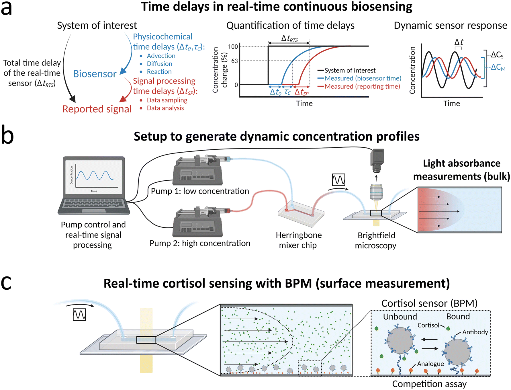 | ||
| Fig. 1 Real-time continuous monitoring of dynamic concentration profiles. (a) Time delays in real-time continuous biosensing. The total time delay of the real-time sensor that monitors the concentration in a system of interest has both physicochemical contributions and signal processing contributions. Physicochemical contributions include transport processes (advection, diffusion) and molecular reactions in the sensor (binding kinetics). The signal processing time delay is determined by the data sampling time and data analysis time. Quantification of physicochemical time delays is performed by applying step functions of concentrations and extracting the transport time delay Δt0 and the characteristic equilibration time τC by single-exponential fitting (see definitions section 2.2). The sketch indicates the total time delay of the real-time sensor ΔtRTS, which is the sum of the physicochemical time delays (Δt0, τC) and the signal processing time delay ΔtSP. The dynamic sensor response is studied by supplying the sensor with sinusoidal concentration profiles. The measured concentration–time profile CM(t) may differ with respect to the concentration–time profile in the system of interest CS(t), in terms of its amplitude and lag time. (b) Setup for generating and measuring dynamic concentration profiles, exemplified with light absorbance measurements of dynamic concentrations of dye molecules. Light absorbance measurements probe the bulk solution in the measurement chamber. The flow rates of pump 1 (containing a low concentration) and pump 2 (containing a high concentration) are continuously controlled by a computer. The output solutions of pump 1 and pump 2 are mixed in a herringbone mixer chip to generate dynamic concentration profiles. The output of the herringbone mixer chip is connected to the biosensor chip that is imaged with brightfield microscopy. Captured images are processed in real time. (c) Real-time continuous biosensing of cortisol with a BPM sensing surface. Measured time delays are related to analyte transport and molecular reactions at the surface. The right panel shows a sketch of a BPM sensor for cortisol, with a competition assay format.25 Particles functionalized with anti-cortisol antibodies are tethered (dsDNA tether) to the sensor surface that is functionalized with cortisol-analogue. The sensing principle is based on the formation of reversible bonds between the antibodies on the particle and cortisol-analogue molecules on the sensor surface. The concentration of cortisol influences the switching between bound and unbound states, since cortisol molecules can bind to the antibodies on the particle, thereby blocking the bond formation between the particle and surface. | ||
2.2 Definitions
The middle panel of Fig. 1a shows that at any moment in time, three concentrations can be identified in the sensing system: (1) the analyte concentration in the system of interest, (2) the concentration that is measured by the biosensor, and (3) the concentration that is reported by the biosensor. The three corresponding concentration–time profiles are correlated in the time-domain according to the following definitions:Transport time delay Δt0,X: the time until a change of concentration is measured in the biosensor after applying a concentration step function in the system of interest, for concentrations measured by method X. In this research we used two methods: light absorbance (X = A) and biosensing by particle motion (X = BPM).
Characteristic equilibration time τC,X: the characteristic time of a single-exponential fit (see eqn (5) and (6)) of the measured concentration–time profile after applying a concentration step function, for concentration measured by method X (see above).
Total physicochemical time delay ΔtC63%,X: time delay due to physicochemical effects to measure 63% of the concentration change after applying a concentration step function, given by:
| ΔtC63%,X = Δt0,X + τC,X | (1) |
 | (2) |
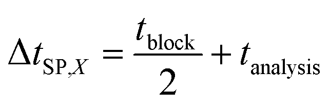
| ΔtRTS,X = ΔtC63%,X + ΔtSP,X | (3) |
2.3 Experimental setup
Fig. 1b illustrates the setup for generating and measuring dynamic concentration profiles (see Fig. S1† for a picture of the setup in the lab).2.4 Light absorbance measurements
Concentrations of dye solution were determined by light absorbance measurements. Pump 1 contained Milli-Q water and pump 2 contained a solution of 2% (v/v) JOLA-RED (food coloring) in Milli-Q water. Images were captured at 120 Hz frame rate with an exposure time of 0.3 ms. In each frame, the transmitted light was calculated by taking the average of all pixel values in the FOV. The real-time response is the average transmitted light in each measurement block of 10 seconds.2.5 Cortisol sensor – biosensing by particle motion (BPM)
Cortisol sensing was performed with a BPM competition immunosensor (see Fig. 1c), that was developed by van Smeden et al.25 The BPM cortisol sensor has been demonstrated for continuous monitoring of cortisol in buffer and in blood plasma.25 The functionalization protocol of the cortisol BPM sensor was the same as described in previous work.27 Therefore, only the main components of the sensor are provided here.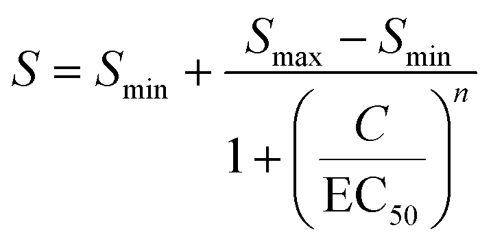 | (4) |
2.6 Single-exponential fitting
Signals and concentrations measured after applying concentration step functions are fitted with single-exponential curves. The function for decreasing signals and concentrations is: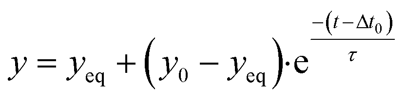 | (5) |
 | (6) |
3. Results and discussion
3.1 Light absorbance measurements
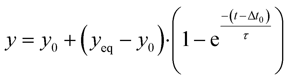
The microfluidic mixing setup for generating dynamic concentration profiles was first studied using light absorbance measurements of fluctuating dye concentrations. These measurements report the average concentration in the measurement chamber along the line of sight and provide the dye transport timescales related to advection and diffusion. Fig. 2a shows a real-time sensing experiment with step functions of dye concentration that were generated by microfluidic mixing. Different concentrations of dye solution were alternated with the baseline concentration (1% of the maximum dye concentration), as sketched in the top panel. The middle panel shows the measured transmitted light intensity. After the inflow of a higher concentration of dye solution the transmitted light intensity decreases as a function of time. The decreases and increases in light intensity are fitted by single-exponential functions (eqn (5) and (6)). The asymptotic values are used to calculate the light absorbance as a function of concentration, as shown in Fig. 2b. The dose–response curve scales linearly according to the Beer–Lambert law. The fitted dose–response relation is used for estimating the concentration in the measurement chamber as a function of time (see Fig. 2a-III).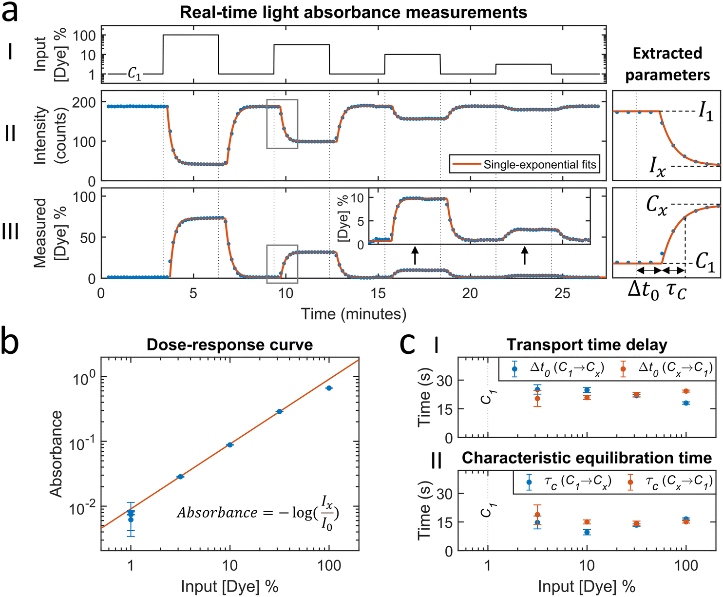 | ||
| Fig. 2 Light absorbance measurements with fluctuating dye concentrations in order to measure timescales related to analyte transport (advection and diffusion). (a) Real-time sensing of dye concentration by light absorbance measurements. (I) Dye concentration as a function of time that was generated by controlled microfluidic mixing. The concentration is expressed as a percentage of the dye solution in pump 2. C1 is the baseline concentration, containing 1% of dye solution. (II) Transmitted light intensity as a function of time. Each datapoint was obtained in real-time (ΔtSP,A ≈ 5 s) and represents the average transmitted light intensity in a measurement block of 10 seconds. Datapoints were fitted with single-exponential curves (eqn (5) and (6)) to extract equilibrium intensity values Ix, that are needed to construct the dose–response curve (panel b). I1 is the equilibrium intensity corresponding to the baseline concentration C1. (III) Measured dye concentration as a function of time. The measured dye concentration (post-processing) was derived from the signal and the fitted dose–response curve (red line in panel b). Datapoints were fitted with single-exponential curves (eqn (5) and (6)), yielding a transport time delay Δt0 and equilibration time τC. (b) Dose–response curve: absorbance as a function of the dye solution percentage. The absorbance values are calculated according to the equation with the fitted equilibrium intensities Ix (panel a) and I0 (blank measurement, data not shown in panel a). The error bars are the 95% confidence intervals of the fitted equilibrium intensities Ix. The red line shows the linear fit, which is according to the Beer–Lambert law. (c) Transport time delay (I) and characteristic equilibration time (II) as a function of the dye solution percentage, obtained from the fitted single-exponential curves in panel a-III. The blue and red datapoints correspond to concentration changes from the baseline towards a higher concentration (C1 → Cx), and from the higher concentration towards the baseline (Cx → C1), respectively. The error bars are the 95% confidence intervals. The mean with standard deviation of the transport time delay is 22 ± 2 seconds. The mean with standard deviation of the characteristic equilibration time is 15 ± 3 seconds. | ||
The concentration time trace is used to extract the transport timescales, by fitting single-exponential curves that are delayed with a transport time delay Δt0,A. The average value of Δt0,A is 22 ± 2 seconds (see Fig. 2c-I), which is the time required for analyte transportation from the mixing chip to the sensor chip. The transport time delay can be influenced by changing the parameters related to the advective sampling, including the tubing length, the dimensions of the sensor chip and the flow rate (Δt0 ∝ V/Q). The time constant of the single-exponential fit τC,A is the characteristic equilibration time, which is dependent on advection and diffusion parameters including the flow profile, the flow rate, the flow chamber dimensions and the diffusion coefficient of the dye molecules. Fig. 2c-II shows that the equilibration time is not dependent on the dye concentration and has an average value of 15 ± 3 seconds.
3.2 BPM sensing under continuous flow
A cortisol BPM sensor was integrated in the microfluidic flow cell in order to study time delays for real-time sensing at a surface in the measurement chamber, as sketched in Fig. 1c. In short, particles with anti-cortisol antibodies were tethered to a surface functionalized with oligonucleotides. Thereafter a solution with cortisol-analogue (cortisol-DNA conjugate) was supplied, causing hybridization of the analogues. The presence of cortisol analogues on the surface causes reversible switching of particles between bound and unbound states. The switching behavior changes when the sensor is exposed to a solution containing cortisol, because the cortisol binds to the antibodies and reduces the probability per unit of time that particles switch from unbound to bound states. In this study we focus on continuous advection-based sampling, which requires that the sensor functions well under continuous flow. In previous BPM studies, the particle switching activity, bound and unbound state lifetimes, and particle bound fraction have been used as readout parameters. Here, the bound fraction (derived from the diffusion coefficient time traces, see ESI† section S2) is used, since it gives robust results under flow.Fig. 3 shows the behavior of the cortisol BPM sensor for various experimental conditions. Before supply of cortisol-analogue molecules, particles mostly show motion patterns of circular shape with a size defined by the length of the dsDNA tether and the particle diameter, see Fig. 3a. On the right hand side, histograms are shown of the diffusion coefficient of a single particle measured over a time span of 30 seconds, and of all particles in the field of view. When a flow is applied from right to left, the particle motion becomes confined due to the fluidic drag force that pushes the particles toward the direction of the flow, resulting in moon-shaped motion patterns and diffusion coefficient histograms that shift to lower values, see Fig. 3b. After hybridization of cortisol-analogue, the particles show state switching behavior that originates from the reversible interaction between the analogue molecules on the sensor surface and the antibodies on the particles, visible without flow (Fig. 3c) as well as with an applied flow (Fig. 3d). Bound states can be recognized in the motion patterns by a higher density of data points in a confined region, and in the time traces by time periods with a reduced variability in x and y. In the presence of flow, a diffusion coefficient threshold is set to separate bound states (red) and unbound states (grey). The fraction of bound states with respect to the total states in the histogram is defined as the bound fraction (BF). During sensor operation, cortisol molecules are present in solution and these bind to the antibodies on the particles, thereby blocking the bond formation between the antibodies on the particles and the cortisol-analogue molecules on the sensor surface, see Fig. 3e. The blocking increases the particle diffusivity and reduces the bound fraction, as shown in the single-particle and the all-particle histograms. The single particle is clearly in the unbound state during the measurement. The all-particle histogram shows overlapping distributions of bound and unbound states, caused by particle-to-particle variations in roughness, tethering, and densities of binder molecules.33,34 To simplify the data analysis, the same diffusion coefficient threshold of 0.033 μm2 s−1 was used in the analysis of all particle time traces in the subsequent experiments.
 | ||
| Fig. 3 BPM sensing with flow. A single particle and an ensemble of particles in a cortisol BPM sensor is studied for various functionalization steps and flow conditions. The shown motion patterns, the time traces, and the histograms marked “single particle”, are all derived from one and the same particle in the cortisol BPM sensor. The particle motion is tracked in x and y direction and visualized as motion patterns and time traces. The diffusion coefficient time trace (D) is derived from the x and y time traces of the particle (see ESI† section S2). In the time traces graphs, the blue arrows indicate a scale of 1 μm and the grey arrows a scale of 0.2 μm2 s−1. The diffusion coefficient values in the time trace of the single particle are shown in the left histogram. The diffusion coefficient histogram of all particles (at the right) combines the diffusion coefficient histograms of all particles in the field-of-view. The bound fraction BF is the real-time signal parameter that is extracted from the diffusion coefficient histograms by setting a threshold (black vertical line at 0.033 μm2 s−1). Diffusion coefficient values below the threshold are classified as bound (red color). (a) Measurements without flow before functionalization of the surface with analogue. (b) Measurements with flow before functionalization with analogue. Flow direction is from right to left, as the pump was in withdrawal mode during the sensor functionalization steps. (c) Measurements without flow after functionalization with analogue. (d) Measurements with flow after functionalization with analogue. Flow direction is from left to right, as pumps were in infusing mode to transport liquid from the syringes to the mixing chamber and measurement chamber. (e) Real-time cortisol sensing with continuous flow, with a cortisol concentration of 30 μM. During the measurement series of panels a to e, the number of particles in the field of view decreased from 1367 to 807; the loss of particles is attributed to flow-induced dissociation31,32 of biotin–streptavidin bonds of the dsDNA tether. | ||
3.3 Real-time cortisol sensing: responses and timescales
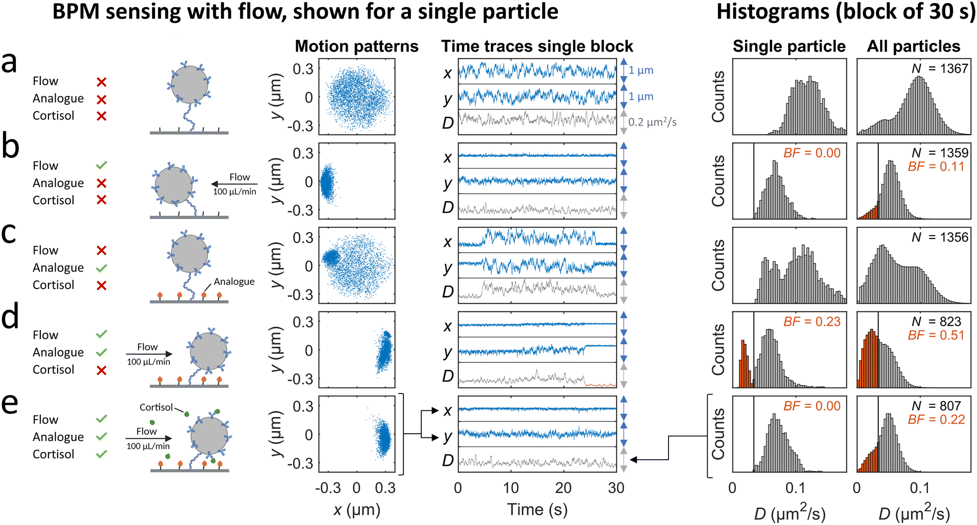
Fig. 4 shows a study on the response of a cortisol BPM sensor to a series of concentration step functions. Fig. 4a shows that a concentration increase gives a rapid decrease of the bound fraction until a stable level is reached. A concentration decrease gives an increase of the bound fraction, with a somewhat slower response. The sensor is reversible as evidenced by the fact that every return to concentration C1 gives the same bound fraction signal, which is discussed in ESI† section 3.2. Fig. 4b shows the bound fraction as a function of the cortisol concentration, which is determined from the equilibrium bound fraction values of the fitted single-exponential curves in panel a. The dose–response relationship is obtained by fitting a sigmoidal function (eqn (4)) to the data. The fitted dose–response relation is used to determine the measured concentration of the BPM sensor as a function of time (see Fig. 4a-III). Large fluctuations are observed in the measured concentration at cortisol concentrations above 10 μM; this can be attributed to the S-shape of the dose–response curve, giving a reduced slope at high concentrations, so that small fluctuations in signal lead to large fluctuations in the measured concentration. With this data, it is possible to determine the transport time delay and characteristic equilibration times, see Fig. 4c. The equilibration time includes contributions of advection, diffusion, and affinity reactions in the BPM sensor. No clear dependence on the analyte concentration is observed in the equilibration time. The average transport time delay and the average equilibration time in the BPM experiments (Δt0,BPM ≈ 32 s, τC,BPM ≈ 37 s) are longer than the parameters in the absorbance experiments in Fig. 2 (Δt0,A ≈ 22 s, τC,A ≈ 15 s). The longer transport time delay in BPM can be attributed to the additional time involved in the transport of analyte towards the sensing surface. The longer equilibration time can be attributed to analyte transport towards the sensing surface and the affinity reactions in the sensor. The resulting total time delay of the BPM sensor for measuring 63% of the cortisol concentration change (ΔtRTS,BPM) is ∼90 s, which is the sum of the physicochemical time delay (ΔtC63%,BPM ≈ 70 s) and the signal processing time delay (ΔtSP,BPM ≈ 20 s). | ||
| Fig. 4 Real-time cortisol sensing. (a) Real-time sensing of cortisol concentrations with BPM. (I) Cortisol concentration as a function of time that was generated by controlled microfluidic mixing. C1 is the baseline concentration of 300 nM (100 times dilution of the 30 μM cortisol solution in pump 2). (II) Bound fraction as a function of time. Each datapoint was obtained in real-time (ΔtSP,BPM ≈ 20 s) and represents the bound fraction in a measurement block of 30 seconds. Datapoints were fitted with single-exponential curves (eqn (5) and (6)). (III) Measured cortisol concentration as a function of time. The measured cortisol concentration (post-processing) was derived from the signal and the fitted dose–response relation (red curve in panel b). The data was fitted with single-exponential curves (eqn (5) and (6)). ESI† section S3.1 provides an additional figure with motion patterns at different cortisol concentrations. (b) Dose–response curve: bound fraction as a function of the cortisol concentration, obtained from the fitted single-exponential curves on the bound fraction (fits were performed on data with a 10 times higher time-resolution, see ESI† section S3.3). The error bars are the 95% confidence intervals. The red curve shows the sigmoidal fit (eqn (4)) with an EC50 value of 2.5 μM and n of 1.3. (c) Transport time delay (I) and characteristic equilibration time (II) as a function of the cortisol concentration, obtained from the fitted single-exponential curves on the measured concentration (fits were performed on data with a 10 times higher time-resolution, see ESI† section S3.3). The blue and red datapoints correspond to concentration changes from the baseline towards a higher concentration (C1 → Cx), and from the higher concentration towards the baseline (Cx → C1), respectively. The error bars are the 95% confidence intervals. The mean with standard deviation of the transport time delay is 32 ± 7 seconds. The mean with standard deviation of the characteristic equilibration time is 37 ± 17 seconds. | ||
The presented experimental approach allows one to determine the total time delay of a real-time sensor and can help researchers to study the effects of changes in sensor design parameters. Estimations of the roles of advection, diffusion, reaction, and signal processing in the present cortisol BPM sensor (see ESI† section S4) indicate that advection and diffusion are the most significant contributors to the total time delay. In a future sensor design, the advection and diffusion timescales could be shortened by decreasing the dimensions of the measurement chamber.
3.4 Sensing sinusoidal cortisol concentration–time profiles
Fig. 5 shows a study on the dynamic response of the cortisol BPM sensor to sinusoidal cortisol concentration–time profiles. The average of the sine functions was set to 3.15 μM, which is close to the EC50 value of 2.5 μM (see Fig. 4b). The amplitude of the sine was set to 2.85 μM, resulting in concentration fluctuations between 300 nM and 6 μM. The periods of the applied sine functions were set to 40, 20, 10, 5 and 2.5 minutes. Before (0–30 min) and after (220–250 min) the sinusoidal modulations, calibration measurements were performed by applying step functions at 300 nM and 6 μM (see ESI† section S5). Calibration was used to correct the dose–response relationship for gradual changes of the sensor, e.g., due to changes of binders on particle or substrate or non-specific interactions.23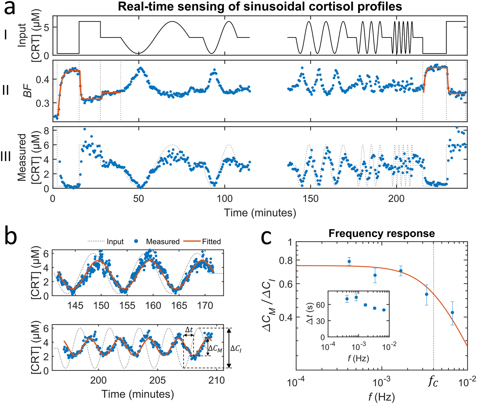 | ||
Fig. 5 Real-time sensing of sinusoidal cortisol concentration–time profiles. (a-I) Cortisol concentration as a function of time that was generated by controlled microfluidic mixing. No data is shown between 120 and 135 min, because in this period the experiment was halted in order to refill the syringe of pump 1. (II) Measured BPM bound fraction as a function of time. Each datapoint was obtained in real-time (ΔtSP,BPM ≈ 20 s) and represents the bound fraction in a measurement block of 30 seconds. Responses obtained after applying step functions were fitted with single-exponential curves (eqn (5) and (6)). Extracted equilibrium bound fraction values were used for calibration, i.e., a correction of the dose–response relation (see ESI† section S5). (III) Measured cortisol concentration as a function of time. The measured cortisol concentration (post-processing) was derived from the signal and the corrected dose–response relation. (b) Two constant-frequency segments of the data in panel a-III. The data is plotted with a 10 times higher time resolution, obtained by splitting each measurement block of 30 seconds into 10 sub-blocks of 3 seconds. The data (blue dots) was fitted with sine functions (red curves), in order to extract the measured concentration change ΔCM and lag time Δt. (c) Frequency response of the studied real-time cortisol sensor. Measured concentration change ΔCM (normalized to the input concentration change ΔCI) as a function of the modulation frequency f. The red curve shows the fit 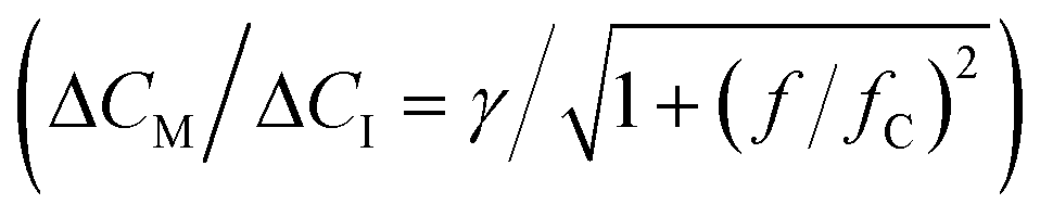 that was applied to extract the cutoff frequency fC, which was found to be ∼4 mHz. The inset shows the lag time Δt as a function of f. that was applied to extract the cutoff frequency fC, which was found to be ∼4 mHz. The inset shows the lag time Δt as a function of f. | ||
Fig. 5a-II shows the real-time sensor signal. The changes in the bound fraction are larger for a concentration decrease (3.15 μM to 0.3 μM) compared to a concentration increase (3.15 μM to 6 μM), which is due to the non-linear dose–response curve. Fig. 5a-III shows the cortisol concentrations derived from the measured bound fractions and the established dose–response curve. Measurements at concentrations above ∼4 μM show more noise than measurements at lower concentrations, because the concentration determination is less precise toward the tail of the S-shaped dose–response curve (see Fig. 4b). The measured concentration–time profiles oscillate with the same frequency as the input concentrations. Fig. 5b shows the sensor responses for the sinusoidal modulations with periods of 10 minutes (top) and 2.5 minutes (bottom), plotted with a 10 times higher time-resolution compared the data in Fig. 5a-III. Sine functions were fitted to this data to determine the amplitude–frequency response of the cortisol sensor, i.e., the measured concentration change ΔCM (normalized to the input concentration change ΔCI) as a function of the modulation frequency f (see Fig. 5c). The amplitude versus frequency data was fitted with the following function:
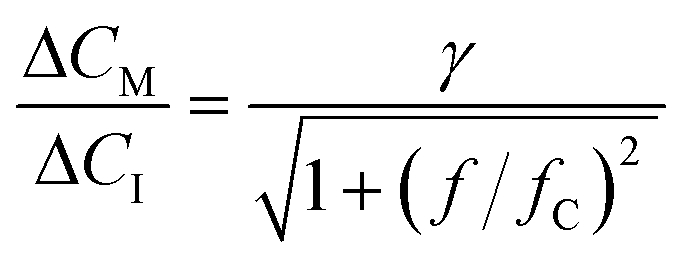 | (7) |
The presented experimental methodology with sinusoidal concentration modulations allows one to test if a biosensor is able to perform continuous monitoring of dynamic concentration changes and clarifies the frequency response of the sensor. It will help researchers to tune sensor design parameters in order to ensure that the sensor is fast with respect to the concentration fluctuations in the system of interest.
4. Conclusions
In this paper we developed an experimental methodology to unravel and quantify the time delays that determine the dynamic response of affinity-based biosensors for continuous sensing. The methodology was demonstrated by continuous monitoring of dynamic cortisol concentration–time profiles with timescales of concentration changes on the order of seconds to minutes. We developed an easy-to-use experimental setup that can generate dynamic concentration profiles with two pumps and a herringbone mixing chip. This experimental approach allowed us to quantify the total time delay of a real-time continuous biosensor, with contributions relating to physicochemical processes (advection, diffusion and reaction) and signal processing. Experiments with the continuous cortisol BPM immunosensor showed a total time delay of about 90 seconds for measuring 63% of an applied concentration change. Monitoring of sinusoidal cortisol concentration–time profiles showed that the sensor has a low-pass frequency response with a cutoff frequency of ∼4 mHz and a lag time of ∼60 seconds.The developed methodologies to quantify time delays and dynamic response can help engineers to design real-time biosensors for applications with diverse analytes, analyte concentrations, and time requirements.13 Studies can be performed on how the dynamic response depends on design parameters of microfluidic systems and molecular designs of continuous sensors. The experimental methodology is also useful for investigating frequency-dependent signal processing concepts such as pre-equilibrium biosensing.28 Detailed experimental studies of the time-dependent behavior of real-time continuous biosensors are expected to lead to novel sensor engineering approaches as well as the development of monitoring-and-control strategies in lab-on-a-chip systems and in biomedical and biotechnological applications.
Author contributions
M. H. B. performed the characterization of the setup with light absorbance measurements. M. H. B. and S. C. performed the cortisol sensing experiments. M. H. B. performed the data analysis. All authors interpreted and discussed experimental results. M. H. B., L. J. v. IJ. and M. W. J. P. co-wrote the paper. All authors approved the submitted version of the manuscript.Conflicts of interest
M. W. J. P. is cofounder of Helia Biomonitoring. All authors declare no further competing interests.Acknowledgements
We thank Stijn Haenen for building the compact imaging setup. Part of this work was funded by the Dutch Research Council (NWO), section Applied and Engineering Sciences, under grant number 16255. Part of this work was funded by the Safe-N-Medtech H2020 project under grant agreement no. 814607. Part of this work was funded by the Consense H2020 project under Marie Skłodowska-Curie grant agreement number 955623.References
- C. Parolo, A. Idili, J. Heikenfeld and K. W. Plaxco, Lab Chip, 2023, 23, 1339–1348 RSC.
- J. Li, J. Y. Liang, S. J. Laken, R. Langer and G. Traverso, Trends Chem., 2020, 2, 319–340 CrossRef CAS.
- K. Scholten and E. Meng, Int. J. Pharm., 2018, 544, 319–334 CrossRef CAS PubMed.
- J. Randek and C. F. Mandenius, Crit. Rev. Biotechnol., 2018, 38, 106–121 CrossRef CAS PubMed.
- B. Wang, Z. Wang, T. Chen and X. Zhao, Front. Bioeng. Biotechnol., 2020, 8, 1–15 CAS.
- C. L. Gargalo, I. Udugama, K. Pontius, P. C. Lopez, R. F. Nielsen, A. Hasanzadeh, S. S. Mansouri, C. Bayer, H. Junicke and K. V. Gernaey, J. Ind. Microbiol. Biotechnol., 2020, 47, 947–964 CrossRef PubMed.
- T. Danne, R. Nimri, T. Battelino, R. M. Bergenstal, K. L. Close, J. H. DeVries, S. Garg, L. Heinemann, I. Hirsch, S. A. Amiel, R. Beck, E. Bosi, B. Buckingham, C. Cobelli, E. Dassau, F. J. Doyle, S. Heller, R. Hovorka, W. Jia, T. Jones, O. Kordonouri, B. Kovatchev, A. Kowalski, L. Laffel, D. Maahs, H. R. Murphy, K. Nørgaard, C. G. Parkin, E. Renard, B. Saboo, M. Scharf, W. V. Tamborlane, S. A. Weinzimer and M. Phillip, Diabetes Care, 2017, 40, 1631–1640 CrossRef PubMed.
- T. Battelino, T. Danne, R. M. Bergenstal, S. A. Amiel, R. Beck, T. Biester, E. Bosi, B. A. Buckingham, W. T. Cefalu, K. L. Close, C. Cobelli, E. Dassau, J. Hans DeVries, K. C. Donaghue, K. Dovc, F. J. Doyle, S. Garg, G. Grunberger, S. Heller, L. Heinemann, I. B. Hirsch, R. Hovorka, W. Jia, O. Kordonouri, B. Kovatchev, A. Kowalski, L. Laffel, B. Levine, A. Mayorov, C. Mathieu, H. R. Murphy, R. Nimri, K. Nørgaard, C. G. Parkin, E. Renard, D. Rodbard, B. Saboo, D. Schatz, K. Stoner, T. Urakami, S. A. Weinzimer and M. Phillip, Diabetes Care, 2019, 42, 1593–1603 CrossRef PubMed.
- D. Rodbard, Diabetes Technol. Ther., 2016, 18, S2-3–S2-13 CrossRef PubMed.
- A. Dillen and J. Lammertyn, Analyst, 2022, 147, 1006–1023 RSC.
- K. W. Plaxco and H. T. Soh, Trends Biotechnol., 2011, 29, 1–5 CrossRef CAS PubMed.
- R. M. Lubken, M. H. Bergkamp, A. M. de Jong and M. W. J. Prins, ACS Sens., 2021, 6, 4471–4481 CrossRef CAS PubMed.
- R. M. Lubken, A. M. de Jong and M. W. J. Prins, ACS Sens., 2022, 7, 286–295 CrossRef CAS PubMed.
- B. S. Ferguson, D. A. Hoggarth, D. Maliniak, K. Ploense, R. J. White, N. Woodward, K. Hsieh, A. J. Bonham, M. Eisenstein, T. E. Kippin, K. W. Plaxco and H. T. Soh, Sci. Transl. Med., 2013, 5, 213ra165 Search PubMed.
- N. Arroyo-Currás, J. Somerson, P. A. Vieira, K. L. Ploense, T. E. Kippin and K. W. Plaxco, Proc. Natl. Acad. Sci. U. S. A., 2017, 114, 645–650 CrossRef PubMed.
- C. Parolo, A. Idili, G. Ortega, A. Csordas, A. Hsu, N. Arroyo-Currás, Q. Yang, B. S. Ferguson, J. Wang and K. W. Plaxco, ACS Sens., 2020, 5, 1877–1881 CrossRef CAS PubMed.
- M. Poudineh, C. L. Maikawa, E. Y. Ma, J. Pan, D. Mamerow, Y. Hang, S. W. Baker, A. Beirami, A. Yoshikawa, M. Eisenstein, S. Kim, J. Vučković, E. A. Appel and H. T. Soh, Nat. Biomed. Eng., 2021, 5, 53–63 CrossRef CAS PubMed.
- I. A. P. Thompson, J. Saunders, L. Zheng, A. A. Hariri, N. Maganzini, A. P. Cartwright, J. Pan, M. Eisenstein and H. T. Soh, bioRxiv, 2023, preprint, DOI:10.1101/2023.03.07.531602.
- A. A. Hariri, A. P. Cartwright, C. Dory, Y. Gidi, S. Yee, K. Fu, K. Yang, D. Wu, I. A. P. Thompson, N. Maganzini, T. Feagin, B. E. Young, B. H. Afshar, M. Eisenstein, M. Digonnet, J. Vuckovic and H. T. Soh, bioRxiv, 2023, preprint, DOI:10.1101/2023.03.03.531030.
- E. W. A. Visser, J. Yan, L. J. van IJzendoorn and M. W. J. Prins, Nat. Commun., 2018, 9, 2541 CrossRef PubMed.
- R. M. Lubken, A. M. de Jong and M. W. J. Prins, Nano Lett., 2020, 20, 2296–2302 CrossRef CAS PubMed.
- J. Yan, L. van Smeden, M. Merkx, P. Zijlstra and M. W. J. Prins, ACS Sens., 2020, 5, 1168–1176 CrossRef CAS PubMed.
- Y. T. Lin, R. Vermaas, J. Yan, A. M. De Jong and M. W. J. Prins, ACS Sens., 2021, 6, 1980–1986 CrossRef CAS PubMed.
- A. D. Buskermolen, Y.-T. Lin, L. van Smeden, R. B. van Haaften, J. Yan, K. Sergelen, A. M. de Jong and M. W. J. Prins, Nat. Commun., 2022, 13, 6052 CrossRef CAS PubMed.
- L. van Smeden, A. Saris, K. Sergelen, A. M. de Jong, J. Yan and M. W. J. Prins, ACS Sens., 2022, 7, 3041–3048 CrossRef CAS PubMed.
- T. M. Squires, R. J. Messinger and S. R. Manalis, Nat. Biotechnol., 2008, 26, 417–426 CrossRef CAS PubMed.
- M. H. Bergkamp, S. Cajigas, L. J. van IJzendoorn and M. W. J. Prins, ACS Sens., 2023, 8, 2271–2281 CrossRef CAS PubMed.
- N. Maganzini, I. Thompson, B. Wilson and H. T. Soh, Nat. Commun., 2022, 13, 7072 CrossRef CAS PubMed.
- A. D. Stroock, S. K. W. Dertinger, A. Ajdari, I. Mezić, H. A. Stone and G. M. Whitesides, Science, 2002, 295, 647–651 CrossRef CAS PubMed.
- K. J. A. Martens, A. N. Bader, S. Baas, B. Rieger and J. Hohlbein, J. Chem. Phys., 2018, 148, 123311 CrossRef PubMed.
- A. Pierres, A. M. Benoliel and P. Bongrand, J. Biol. Chem., 1995, 270, P26586–P26592 CrossRef PubMed.
- A. Pierres, D. Touchard, A. M. Benoliel and P. Bongrand, Biophys. J., 2002, 82, 3214–3223 CrossRef CAS PubMed.
- R. M. Lubken, A. M. de Jong and M. W. J. Prins, ACS Nano, 2021, 15, 1331–1341 CrossRef CAS PubMed.
- E. W. A. Visser, L. J. van IJzendoorn and M. W. J. Prins, ACS Nano, 2016, 10, 3093–3101 CrossRef CAS PubMed.
Footnote |
| † Electronic supplementary information (ESI) available. See DOI: https://doi.org/10.1039/d3lc00410d |
| This journal is © The Royal Society of Chemistry 2023 |