
 Open Access Article
 This Open Access Article is licensed under a
 Creative Commons Attribution 3.0 Unported Licence
Machine learning analysis to classify nanoparticles from noisy spICP-TOFMS data†
Raven L.
Buckman
 and
Alexander
Gundlach-Graham
*
and
Alexander
Gundlach-Graham
*
Department of Chemistry, Iowa State University, Ames, Iowa, USA. E-mail: alexgg@iastate.edu
First published on 16th May 2023
Abstract
Single-particle inductively coupled plasma time-of-flight mass spectrometry (spICP-TOFMS) is a promising method for the quantification and classification of anthropogenic and natural nanoparticle (NP) types based on measured multi-elemental compositions of individual particles. However, spICP-TOFMS data shows systematic bias in the detected elemental compositions of particles as a function of particle size, composition, and analytical sensitivity. To overcome the inherent bias of spICP-TOFMS data for the classification of NP types, we report a multi-stage semi-supervised machine learning (SSML) strategy. In our approach, systematic particle misclassifications are first found and then these “noise classes” are incorporated into the SSML model for the development of a second, more robust classification model. As a case study, we use cerium(IV) oxide, ferrocerium mischmetal, and bastnaesite mineral NPs as representatives for engineered (ENP), incidental (INP), and natural (NNP) nanoparticle types, and classify particles in mixed samples based on our final SSML model. This two-stage SSML model has a receiver operating characteristic area under the curve (ROC AUC) value of 0.979, and false-positive rates of 0.030, 0.001 and 0 for ENPs, INPs and NNPs, respectively. These low false-positive rates allow for accurate particle-type classification of mixed samples with variable number concentrations; here, we demonstrate particle-type quantification across more than two orders of magnitude. Overall, our two-stage SSML model for NP classification identifies and overcomes bias in spICP-TOFMS training data to provide a simple and robust approach for incorporation of machine learning models in spICP-TOFMS particle classification strategies.
Introduction
Nanoparticles (NPs) and microparticles (μPs) are ubiquitous in the environment; however, anthropogenic nanomaterials have been, and continue to be, introduced into ecological habitats as a result of human activity.1–5 For example, NPs can be found in a variety of consumer products such as cosmetics, food, and fuels; particles from these products are ultimately released, unknowingly or otherwise, into the environment as a byproduct of our everyday lives.6,7 To characterize NPs in consumer products and environmental samples, we must consider a variety of features including particle size, morphology, elemental composition, and sample matrix because available analytical techniques can only, at best, measure a few features.8–10 Cohesive and comprehensive quantification of NPs is challenging due to varying measurement parameters, varying data analysis processes, and differences in the metrics reported. Nanoparticles are analyzed with a wide variety of methods such as atomic force and electron microscopy, dynamic light scattering, separation approaches combined with inductively coupled plasma mass spectrometry (ICP-MS), and single-particle ICP-MS.11Recently, single-particle inductively coupled plasma time-of-flight mass spectrometry (spICP-TOFMS) has become a robust analytical tool for nanomaterial characterization.12,13 To measure individual particles, mass spectra are collected at high-time resolution (∼1 ms or lower) and single-particle events are recorded as signal spikes that deviate from a well-characterized steady-state background.14 This high-throughput method enables multi-elemental analysis of short transient signals with high absolute sensitivity.15,16 With spICP-TOFMS, researchers can accurately count and determine the elemental mass amounts from particles ranging between ∼10 to 2000 nm in diameter (assuming a spherical shape, and depending on particle density and elemental composition).17 These fundamental features of spICP-TOFMS make it an ideal technique for the quantification and characterization of multi-elemental NPs and μPs.
spICP-TOFMS has been used to quantify sample suspensions from (among others) surface waters,18 soils and sewage,19 snow aerosols,20 road run off,21 and space-station aerosols.22 Other methods of single-particle quantification have been performed for similar environmental samples using spICP-MS with triple quadrupole,23–25 single quadrupole,26–28 or sector-field18 mass analyzers. While it can be challenging to determine and confirm the originating source of NPs, at elevated concentrations, long-term field studies have shown temporal variations of NP concentration as a function of weather patterns29–31 and/or human activity.25 Previous studies have also used a variety of methodologies to characterize NP events for source apportionment.1,18,19,21,23,25,27,32–38 For spICP-TOFMS analysis, particle classification has been performed with supervised and unsupervised machine learning, among other methods, because of the potential for automated labelling and classification, thus, reducing the analysis time.21 Examples of supervised learning methods used for NP and μP classification from spICP-TOFMS datasets include gradient boosted classifiers (GBC),32 light-GBC,21k-nearest neighbor embedding (KNN),35 and binomial logistic regression (LR).19 Unsupervised approaches, such as clustering analysis20,33,34,39 or t-stochastic neighbor embedding,21 have also been reported for NP classification from spICP-TOFMS datasets.
Semi-supervised machine learning (SSML) algorithms are a subclass of machine learning that combine supervised and unsupervised learning approaches40 with the intention of improving the performance of one task with information from the other.40–44 SSML algorithms are particularly relevant to scenarios where labelled data is scarce and unlabeled data is abundant. However, SSML methods can also be applied in circumstances where labelled data is abundant if the unlabeled data provides additional information relevant to future predictions.42–44 Either of these circumstances could be the case for spICP-TOFMS data. For spICP-TOFMS data analysis, we need robust classification models that can predict NP classifications from real samples. These models should not be bound by stringent classification boundaries19 inherent to supervised learning and should be able to recognize similarities or differences across predictors,21 as would be accomplished with unsupervised learning methods.40,41,45–47 One specific taxonomy of SSML that could be particularly useful for NP classification from spICP-TOFMS data is that of a self-training model, which uses inductive reasoning to build a classification model and iteratively re-trains the model using the most confident predictions.42,48,49 Self-training SSML algorithms, as well as other wrapper methods, are advantageous because they can be used with a wide variety of supervised base learners.42,43 In spICP-TOFMS analyses, there can be significant differences between training data and sample data that impedes supervised ML classification methods; any deviations in particle size distributions, elemental sensitivities, detectable masses, or particle presence can lead to false classifications with supervised ML models. Using a self-training SSML model allows for the model to extrapolate beyond the training data, which enhances the performance of the supervised base learning algorithm.21,42–44
Machine learning models do not always produce logical or interpretable results, especially for data structures with high variability. In spICP-TOFMS, the low signals recorded for small NPs lead to variable and biased detection of elemental presence and ratios; this can complicate the classification of NPs based on elemental fingerprints. To overcome the limitations of noisy spICP-TOFMS measurements, we developed a two-stage semi-supervised machine learning model that uses a first SSML training to refine particle class assignments and develop new model-guided particle classes and a second, subsequent, SSML model for robust particle classification.
Materials and methods
Nanoparticle suspensions
Neat suspensions of CeO2 engineered NPs (ENPs), ferrocerium mischmetal incidental NPs (INPs) and bastnaesite/parisite mineral natural NPs (NNPs) were prepared according to a previous method.37 All suspensions were prepared and diluted in DI water (18 MΩ cm) with 5 ng mL−1 Cs (Cs–water); Cs was used as an uptake standard to determine the solution flux into the plasma (qplasma, mL s−1) for the measurement of particle number concentrations (PNCs) via online microdroplet calibration.50 A 50 mL stock suspension of CeO2 ENPs was prepared using ∼8.4 mg of CeO2 nanopowder (Sigma-Aldrich, MO, USA); serial dilutions were then performed until reaching a final PNC of ∼3.0 × 10⁵ (particles per mL) (Table S1†). A 25 mL stock suspension of INPs was prepared on the day of the experiment by striking a ferrocerium mischmetal-containing disposable lighter (BIC®, CT, USA) 30 times over a beaker containing Cs–water; serial dilutions were then performed until reaching a final PNC of ∼3.4 × 10⁵. A previously prepared stock suspension of milled bastnaesite/parisite mineral powder in water was used in this study and diluted with Cs–water to a final PNC of ∼7.7 × 10⁵. To prepare mixture samples, aliquots of the neat suspensions were added to 4 mL vials; these samples were named and prepared according to Table S2.†Nanoparticle suspensions of ENPs, INPs, NNPs, and mixture samples were analyzed using an icpTOF-S2 instrument (TOFWERK AG, Thun, Switzerland) equipped with an online microdroplet calibration system, as described previously.51,52 Sample aliquots were injected with a microFAST MC autosampler and a PFA pneumatic nebulizer (PFA-ST, Elemental Scientific, NE, USA) connected via a baffled cyclonic quartz spray chamber to the injector of the ICP torch. Additional instrument parameters are provided in Table S3.† Single-particle measurements were conducted with an average-spectrum acquisition time of 1.2 ms. The isotopic signals extracted from the mass spectra, droplet concentrations, and absolute sensitivities used in the quantification of element masses in NPs with online microdroplet calibration are reported in Table S4.† Data from the single-particle experiments were processed using “Time-of-Flight Single-Particle Investigator” (TOF-SPI), an in-house LabVIEW program (LabVIEW 2018, National Instruments, TX, USA). TOF-SPI is designed for processing spICP-TOFMS data combined with online microdroplet calibration; it offers automated determinations of element-specific backgrounds, critical values, absolute sensitivities (Tof Counts [Tof Cts] per g), solution uptake rates, particle intensities (Tof Cts), and element masses (grams, g) per particle. In this work, measured element masses were used for machine learning analysis.
Machine learning
Various supervised machine learning models were tested as a comparison to other methods found in the literature; details are summarized in the ESI (Table S5).† Semi-supervised machine learning (SSML) was performed using MATLAB R2022a (MathWorks Inc., MA, USA) with the Statistics and Machine Learning Toolbox™ (ver. 12.2); a workflow describing the analysis is provided as Fig. S1.† Element mass data was preprocessed to remove all non-Ce-containing particle events from the dataset. Training data for machine learning applications should be as balanced and unbiased as possible; therefore, we randomly selected, with replacement, equal numbers of particle events from each of the three pristine particle type datasets to use for the labeled training set. These randomly selected particle events were concatenated into a single data table and assigned classification labels matching the pristine sample from which they originated (herein referred to as the ‘true class’). An additional unbalanced data table with all Ce-containing particle events from all three particle types was used as the unlabeled data set. The same method was used to train a second SSML model with the same parameters as the first; the only difference between the first and second model is the number of classes used. An example of the code used for analysis can be found on our group's GitHub page (https://github.com/TOFMS-GG-Group).After the labeled and unlabeled datasets were prepared, the tables were read into the fitsemiself function in MATLAB.53 In 1995, David Yarowsky introduced an unsupervised algorithm for word sense disambiguation that rivaled supervised methods.48,49 The Yarowsky algorithm is the basis for the semi-supervised machine learning (SSML) function used here. In SSML, training data is assembled using a small portion of data with labels based on user-defined classifications and a larger portion of unlabeled data.42–44,47,54 To begin training the SSML, a preliminary supervised ML model is constructed using the labelled data. The supervised ML model is then used to predict classes for the unlabeled data; the scores of the predicted labels are compared to a threshold value and the model is iteratively retrained until the scores are above the threshold or the iteration limit is reached. This function has default machine learning parameters such as a limit of 1000 iterations and no binning of predictors. We used a classification type ensemble template as the basis for the semi-supervised model with specified parameters such as a bagging method, 500 learning cycles, and a reproducible decision tree learner type; other parameters can be found in Table S6.† More detailed explanations of the parameters can be found in the MATLAB documentation center (fitsemiself (https://www.mathworks.com/help/stats/fitsemiself.html?searchHighlight=fitsemiself%26s_tid=srchtitle_fitsemiself_1), templateEnsemble (https://www.mathworks.com/help/stats/templateensemble.html?s_tid=doc_ta), templateTree (https://www.mathworks.com/help/stats/templatetree.html?searchHighlight=templateTree%26s_tid=srchtitle_templateTree_1)).
Results and discussion
spICP-TOFMS data analysis
spICP-TOFMS measurements produce rich datasets containing a mixture of single-element and multi-elemental particle events. In spICP-TOFMS, transient signals (Fig. S2†) are identified as coming from individual particles when they are above element-specific critical values (LC,sp) that depend on dissolved background levels and ion-detection response functions of the mass analyzer.14,55–57 While NP signals are found in the signal domain, the critical mass (XmassC,sp) is determined by calibration using element specific sensitivities (Tof Cts per g). When considering the detection of multi-metal nanoparticles (mmNPs), the likelihood of recording certain elemental combinations depends not only on element-specific critical masses, but also on the size distribution and the element mass fractions of a given particle type. For a conserved particle type, more particle events are recorded for elements with high mass fractions and/or low critical masses compared to elements with low mass fractions and/or high critical masses. This means that particle types that are compositionally homogenous, but variable in size, will produce spICP-TOFMS events that have fragmented elemental signatures, i.e. we record a range of single-metal (sm) and mmNP types. More elements will be detected in large particles than small ones and the complexity of the recorded mmNP signatures (compared to the true mmNP composition) complicates the interpretation of spICP-TOFMS data.Mass spectra of the three particle types (Ce-ENPs, -INPs, -NNPs) can be found in Szakas et al. (2022).37 These three NP types have distinct elemental compositions at the population level (see Fig. 1). However, at the single-particle level, some smNP and mmNP elemental signatures overlap. Specifically, CeO2 ENPs produce only Ce smNPs signatures. Ferrocerium mischmetal INPs produce both smNP and mmNP particle events composed, predominantly, of Ce and La; the detected elemental signatures of INPs are shown in Fig. 1A. Bastnaesite NNPs produce particle events with smNP and mmNP signatures with an increased elemental complexity not observed in either the ENPs or INPs (see Fig. 1B). From the NNP sample, smNPs of Ce and La as well as mmNP signatures containing Ce, La, Nd, Pr, Th, and combinations thereof are measured. The overlap of elemental signatures between the NP types reduces the efficacy of some elemental signatures as distinguishable characteristics. The Ce-only elemental signature is found in 100% of ENPs, 48.2% of INPs, and 18.6% of NNPs. Because Ce-only particle event signatures are present in all three NP types, we cannot solely rely on the presence of Ce-only particles for classification of these NP types. Likewise, CeLa-mmNP events are recorded for both the INP and NNP types; whereas 47.1% of the measured signals from the INPs are CeLa-mmNP, 13.3% of the bastnaesite NNP mineral signals carry this signature. These joint elemental signatures complicate the classification of particle events by composition and limits the possibility of using unsupervised ML analysis alone for classification of these Ce-containing particle types (see Fig. S3†). Here, we implement a two-stage SSML approach to identify and overcome the overlap of elemental signatures between particle types for accurate particle classification.
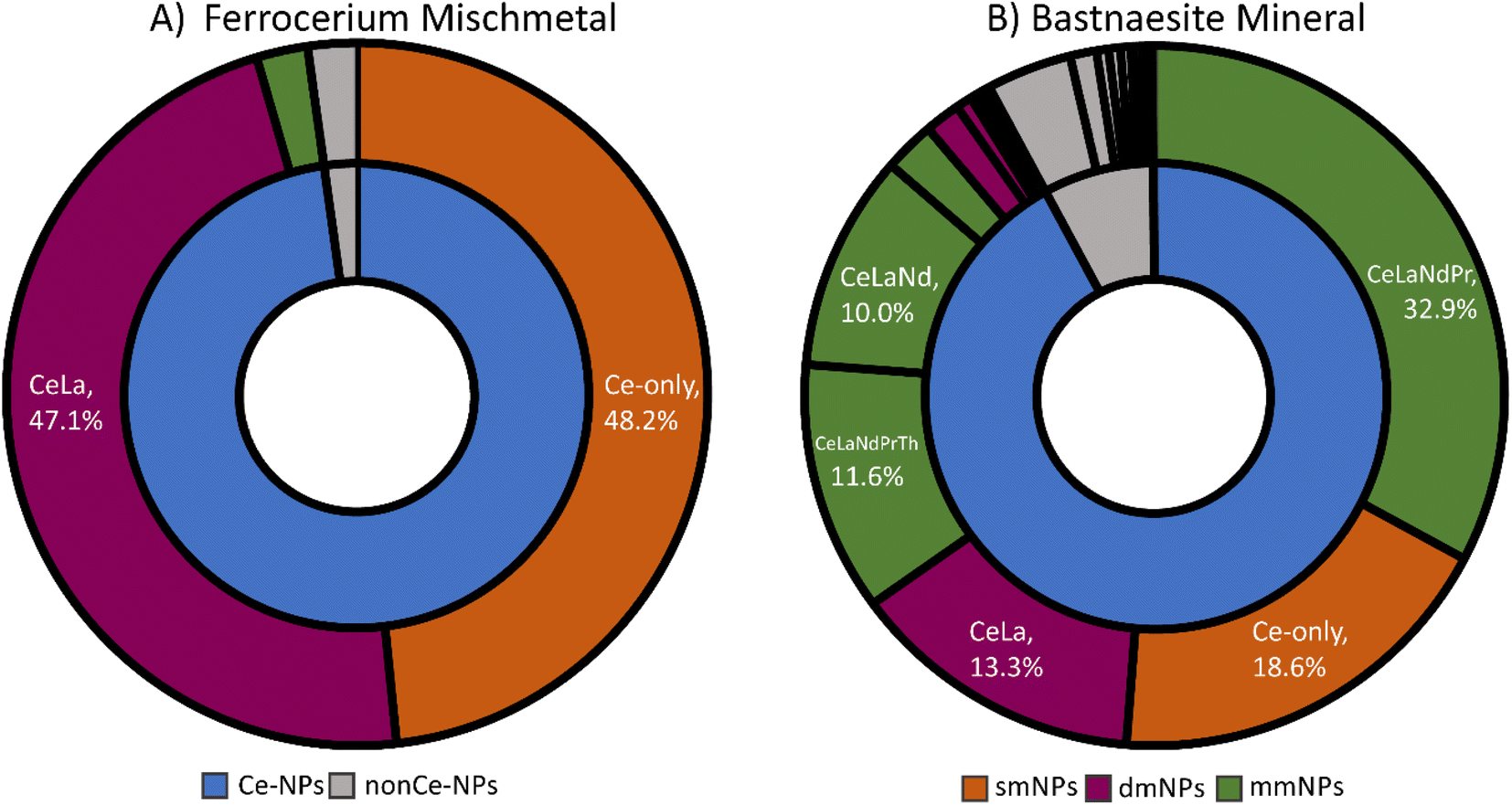 | ||
| Fig. 1 Sunburst plots of the detected elemental signatures of (A) ferrocerium mischmetal NPs and (B) bastnaesite mineral NPs. The grey regions of the plots are particle signals without Ce detected; these are not used in SSML classification. In the inner ring, the blue regions of the plots are Ce-containing particles. In the outer ring, the orange regions are single-metal nanoparticles (smNPs), the plum regions are dual-metal nanoparticles (dmNPs) and the green regions are multi-metal nanoparticles (mmNPs). | ||
Semi-supervised machine learning
To prepare the element mass data for machine learning, we truncate the data at the single-particle critical mass of Ce for the ferrocerium sample (XmassC,sp,Ce,INP, 49.0 ag); all particle signals with Ce mass below this value are not used in the ML analysis. Performing this truncation reduces the impact of run-to-run fluctuations in background signal levels and sensitivities for ML-based classification. The critical mass of Ce from the Ce-INP sample was selected because it is the largest critical mass value for Ce of the three standard particle suspensions. When a real, mixed sample is analyzed by spICP-TOFMS, elements in all the NP types in that sample are detected at the same critical values. Therefore, creating an initial training set with a conserved critical mass mimics the conditions of a mixed sample. Without this data truncation, particles with Ce mass below XmassC,sp,Ce,INP are classified exclusively (and likely falsely) as Ce-ENPs or Ce-NNPs because the semi-supervised machine learning model is not trained to classify NP signatures with low Ce mass as INPs.For semi-supervised machine learning, a relatively small, labeled training set and a larger unlabeled training set are required. The labeled training data set is generated using the neat particle suspensions of CeO2, ferrocerium mischmetal, and bastnaesite mineral. Particle events from each of the three particle types are randomly sampled with replacement 400 times and a ‘true class’ is assigned to each event; these true classes are ENP, INP, or NNP. The unlabeled training set is generated by concatenating all the measured particle events with Ce mass above XmassC,sp,Ce,INP without any assigned classes. The classification ML model is trained using the parameters specified in Table S6.† To test the SSML model performance, we predict classes for the labeled training data and compare the predicted classes to the true classes; the confusion matrix for this first SSML is shown in Fig. 2A.
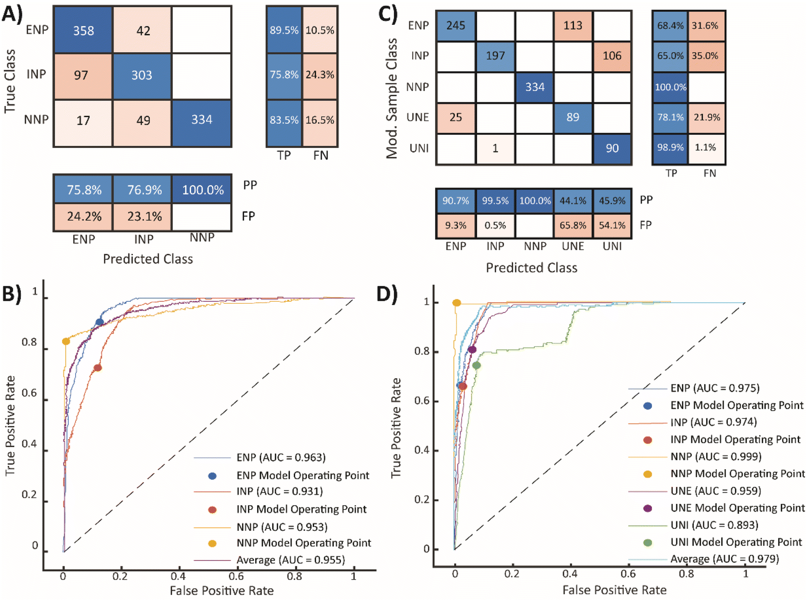 | ||
| Fig. 2 Results from the first and second SSML models. Confusion matrices (A and C) summarize the classification performance of the first and second SSML models, respectively. The row summary (row-normalized) describes the percentage of true-positives (TPs) and false-negatives (FNs). The column summary (column-normalized) is representative of the percentage positive-predictions (PPs) and false-predictions (FPs). The ROC curves (B and D) provide a numeric comparison of the model performance with AUC being a scalar quantity for the first and second SSML models characterization, respectively. | ||
In the confusion matrix in Fig. 2A, the number of particle events whose predicted class matched the true class are shaded blue (true-positives, TPs, and positive-predictions, PPs); the red squares are from particle classifications that did not match the true class (false-predictions, FPs, and false-negatives, FNs). This confusion matrix demonstrates that the SSML model best classifies NNPs, followed by ENPs and INPs. However, the model falsely predicts 24.3% of incidental particles as ENPs. Likewise, 16.5% of NNPs are falsely classified as ENPs or INPs. Using eqn (1), we can calculate the false-positive rate (FPR) by dividing the number of FP classifications by the sum of the FPs and the number of particle events whose classifications are correctly predicted as negative (true-negatives, TNs) for each particle class. The FPRs for the first SSML model are 0.143, 0.114, and 0 for ENPs, INPs, and NNPs, respectively. The accuracy of this model is 0.892; this is calculated by dividing the number of TPs by the total number of particle events. In addition to a confusion matrix, a receiver operating characteristic (ROC) curve is used as a two-dimensional visualization of classification performance (see Fig. 2B). A scalar quantity of the area under the ROC curve (AUC) is used as a gauge for the model performance; the closer an AUC value is to 1, the better the ML model classification performance. For this first stage in the SSML scheme, the weighted-average AUC value is 0.955. Other figures of merit for this model can be found in Table 1. In the ESI,† we also provide precision–recall curves as an additional metric to assess model performance of imbalanced training data,58 for our SSML model (see Fig. S5†); we find the performance assessment with ROC- and PR-based approaches to be similar.
 | (1) |
| Metric | ENP | INP | NNP | UNE | UNI |
|---|---|---|---|---|---|
| Model 1 | |||||
| ACC | 0.829 | N/A | |||
| ROC AUC | 0.963 | 0.931 | 0.953 | ||
| FPR | 0.143 | 0.114 | 0.000 | ||
| Sensitivity | 0.895 | 0.758 | 0.835 | ||
| Specificity | 0.858 | 0.886 | 1.000 | ||
| Precision | 0.759 | 0.769 | 1.000 | ||
| F-measure | 0.821 | 0.763 | 0.910 | ||
![[thin space (1/6-em)]](https://www.rsc.org/images/entities/char_2009.gif) |
|||||
| Model 2 | |||||
| ACC | 0.796 | ||||
| ROC AUC | 0.975 | 0.974 | 0.999 | 0.959 | 0.893 |
| FPR | 0.030 | 0.001 | 0.000 | 0.104 | 0.096 |
| Sensitivity | 0.684 | 0.650 | 1.000 | 0.781 | 0.989 |
| Specificity | 0.970 | 0.999 | 1.000 | 0.896 | 0.904 |
| Precision | 0.907 | 0.995 | 1.000 | 0.441 | 0.459 |
| F-measure | 0.780 | 0.786 | 1.000 | 0.563 | 0.627 |
To employ a machine learning model for particle classification from spICP-TOFMS measurements of real, possibly environmental, samples, the model must be robust enough to accurately predict labels for engineered particles in a relatively high natural background. As such, a machine learning model with false positive rates of 14.3% and 11.4% for ENPs and INPs, respectively, is less than ideal. Suppose an environmental sample is measured with spICP-TOFMS and 10000 Ce-particle events are detected: 9000 of these particles are of natural origin and 1000 events are from Ce-ENPs. Based on the first SSML model, we would predict that ∼400 particle events will be misclassified as ENPs and ∼1200 particle events would be misclassified as INPs. These misclassifications would cause the number concentration of ENPs to be overestimated by ∼30% and the PNC of INPs to be spuriously high. The impact of false-positive ENP and INP classifications increases as the number ratio of natural-to-anthropogenic particles increases, which is what we expect in natural systems. If we implement a classification model with 14.3% false-positives, then we will over-classify engineered and incidental particles and thus report false, systematically biased, contamination levels of anthropogenic particles. Moreover, the true percentage of misclassification from a real sample would be difficult to ascertain due its dependence on particle size distributions and critical masses for all elements. With this in mind, we claim that robust machine learning classification models should aim to reduce false-positive predictions of ENPs and INPs.
To better understand the origin of misclassifications from the first stage of the SSML classification, the individual particle event classifications are plotted as a function of the Ce mass and number of elements detected per particle in Fig. 3. These predicted classifications are directly compared to the Ce mass histograms of the neat suspensions in Fig. 3B; because data for ML is truncated at XmassC,sp,Ce,INP, no particle events below 49 ag are shown in Fig. 3A. From Fig. 3, it is apparent that the first SSML model predicts that the smallest smNPs detected from all three particle types are INPs while more moderately sized smNPs are classified as ENPs. The model also exhibits a similar trend for dual-metal NNPs, which are falsely classified as INPs. These systematic misclassifications indicate that there is an underlying mass distribution dependence within the SSML model.
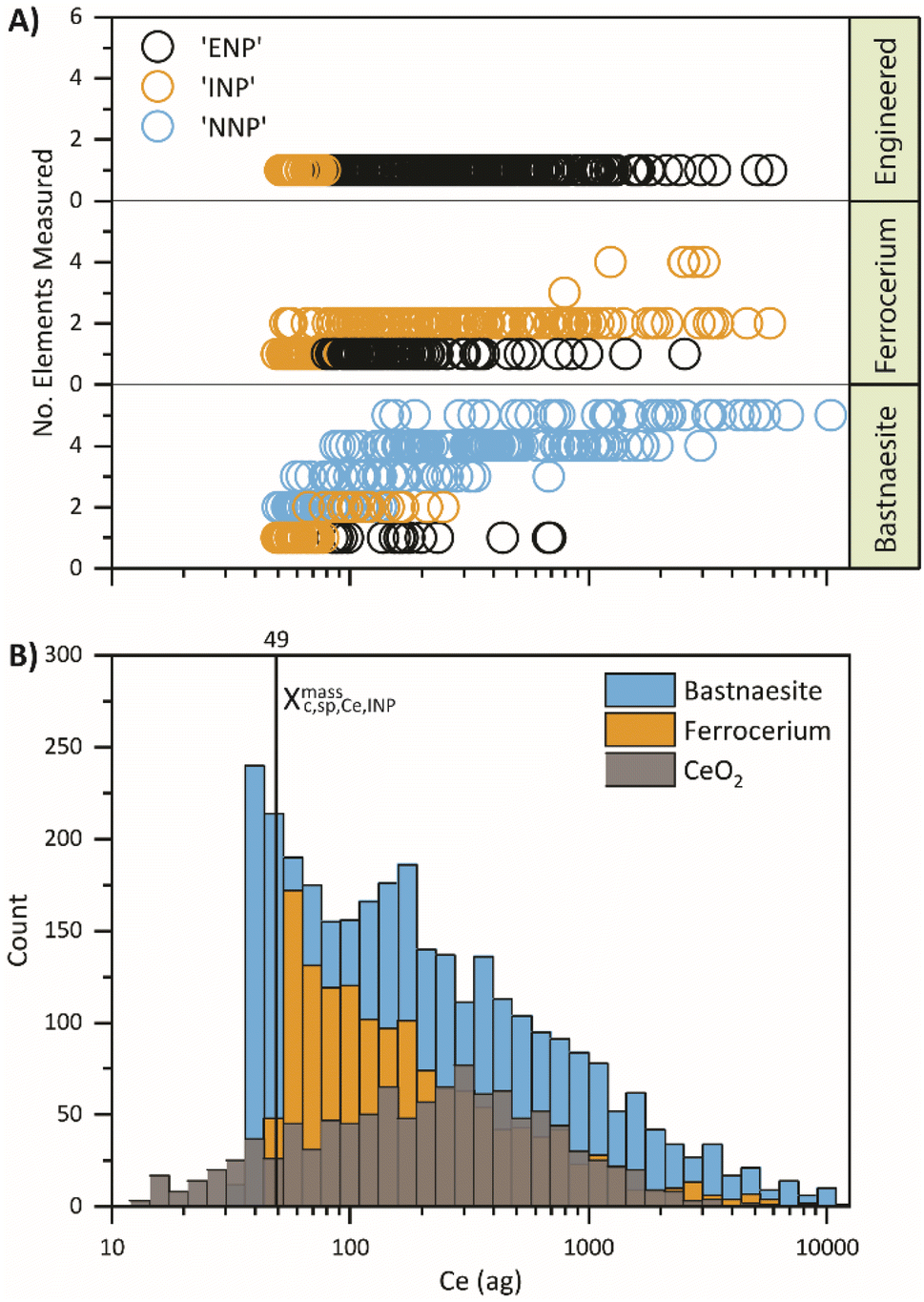 | ||
| Fig. 3 Comparison of particle classification from the first SSML model to the mass distribution of Ce. (A) Individual particle events are plotted by the number of elements detected and grouped vertically by the true particle class as a function of Ce mass (ag). Bubbles are colored by the predicted classification. (B) The mass distribution of each of the three pristine samples; the vertical line indicates XmassC,sp,Ce,INP. | ||
The masses of Ce in CeO2 NPs reveal a skewed log-normal distribution,59 where the mass bin with the highest frequency is centralized with tails on either side. In contrast, ferrocerium mischmetal and bastnaesite mineral NPs exhibit a distribution resembling Weibull60 or two-parameter log-normal61 distributions with the highest frequency mass bin at approximately the critical mass and a right tail. Differences in the shape of the detected mass distributions clearly affects the performance of the SSML. For example, smNPs with moderate Ce mass (∼100–1000 ag Ce) are most probably ENPs because most of the mass distribution of ENPs encompasses this mass range. Likewise, most bastnaesite and ferrocerium NPs have more complex mmNP signatures over the same Ce-mass range. Conversely, the SSML model predicts smNPs with low Ce mass (<∼100 ag Ce) to be most probably INPs because the ferrocerium mischmetal mass distribution is at its highest frequency over this Ce-mass range and many of these small INPs are detected as Ce-smNPs. The systematic misclassification of ENPs and INPs indicates that the mass distributions of given NP types heavily impacts the ML model and introduces a bias that must be corrected. Since misclassified particle events appear grouped as a function of Ce mass, these particle events may be considered distinct unclassifiable particle types (i.e. UNPs) that can be incorporated into the SSML model to counteract the bias that would otherwise be present with a single training.
To account for FP biases in our ML model, we introduce two additional particle classes prior to training a second SSML model; these classes are assigned to the falsely classified particle events used in the initial training set. Particles that were falsely classified as ENPs are relabeled as ‘unclassifiable engineered’ (UNE); these particles are mostly small (low-mass) incidental and natural smNPs. Particles that were falsely classified as INPs are relabeled as ‘unclassifiable incidental’ (UNI); these particles are mostly natural dual-metal (CeLa) NPs. In the second SSML model, each particle class (ENP, INP, NNP, UNE, and UNI) is resampled with replacement 400 times to ensure that the training data is numerically balanced. The same unlabeled dataset, model parameters, and performance metrics are used for the first and second SSML models; results are shown in Fig. 2.
In Fig. 2C, we show the normalized confusion matrix for the second SSML model, in which the values of the matrix are weighted to account for resampling; the non-normalized confusion matrix is shown in Fig. S4.† Correcting for resampling enables a more accurate comparison between predicted classifications and sample types, i.e. PP and FP percentages. Classification with the second SSML model results in 31.6% and 35.0% of ENPs and INPs classified as UNEs and UNIs, respectively. Lower percentages of UNEs and UNIs are falsely predicted to be ENPs or INPs. The ACC of the second SSML model is 0.796; other figures of merit can be found in Table 1. The accuracy of the second SSML model is slightly worse than the first model; however, accuracy can be a misleading statistic for model performance due to the accuracy paradox, and should not be the only metric used to compare the two models.62,63 For our analysis, one of the most important metrics to consider when assessing ML model performance for NP classification is the false-positive rates (FPRs) for each particle type. The FPRs for the second ML model are calculated to be 0.030, 0.001, 0, 0.104, and 0.096 for ENPs, INPs, NNPs, UNEs, and UNIs, respectively. We are most interested in the FPRs for the three original particle classes, as the UNEs and UNIs are “noise” classes. The second ML model demonstrates ∼79% and ∼99% fewer false-positive particle assignments compared to the first SSML model for ENPs and INPs, respectively. This reduction in false-positive classifications enables improved limits of classification of in terms of PNCs for samples with unknown numbers of Ce-NP types. In turn, this will result in lower systematic over-classification of anthropogenic PNCs in NNP-rich samples.
A visual comparison of the classification performance of both models is provided in Fig. 4. In this figure, data points are plotted according to the Ce mass with events grouped vertically by the true particle class, colored by the predicted class, and sized proportional to the number of elements detected in each particle. When comparing classification accuracy between the first (Fig. 4A) and second (Fig. 4B) stage of SSML classification, it is clear that most incorrectly classified ENP and INP particles are accounted for by the UNE and UNI particle classes of the second SSML model. Furthermore, Fig. 4B shows that the second SSML model imposes a kind of mass cutoff for accurate classification of ENPs and INPs, which is akin to particle-type detection limits previously reported.37 As seen in Fig. 2B, the SSML model predicts that Ce-smNPs and dual-metal CeLa-NPs can be classified most accurately as ENPs or INPs, respectively, above a Ce mass of ∼200 ag. Below this mass of Ce, the Ce-smNP and CeLa-mmNPs are more likely to be classified as UNEs or UNIs. These Ce-mass cutoffs are not strict rules, like in detection limit filtering, but rather are the result of a complex decision tree ensemble developed via the SSML modelling.
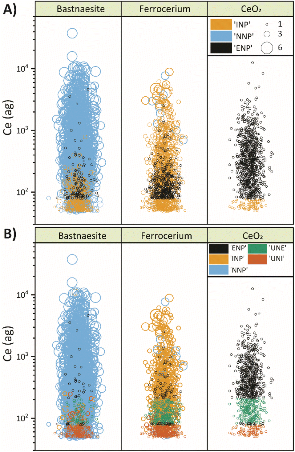 | ||
| Fig. 4 Comparison of the particle classification performed by the first stage (A) and second stage (B) of semi-supervised machine learning. Bubble size is proportional to the number of elements detected in each particle event. Bubbles are divided by the true particle class and colored based on the predicted particle class. | ||
Mixture sample classification
To assess the robustness of the SSML model for accurate quantification, two scenarios are tested by mixing aliquots of ENPs, INPs, NNPs at variable number ratios (see Fig. 5). In the first scenario (Fig. 5A), we increase the concentration of ENPs against a constant background of INPs and NNPs. In the second scenario (Fig. 5B), the concentration of INPs is increased against a constant background of ENPs and NNPs. In an ideally performing classification model, a scatter plot of the number of particles classified versus the predicted particle number would have a slope equal to one for the particle type with changing concentration and the recorded numbers of the other two particle types would have slopes equal to zero. In Fig. 5, it is clear that 100% recovery is not achieved for either the ENPs or the INPs, as slopes of ∼0.45 and ∼0.41 were obtained for dilutions of the two particle types; this reduced sensitivity is expected because many ENP and INP particles are too small to be accurately classified. Nonetheless, the trend of both particle types is linear with slopes significantly different than zero. We performed an ANOVA test to determine whether the linear fit of each classification was significantly different from zero at the 95% confidence level. Trendlines and data for all particle classes can be found in Fig. S6† with results from the ANOVA tests are shown in Table S7.† In Fig. 5A, the slope of the trendline for increasing the PNC of ENPs in the mixture is significantly different from zero while the slopes of the INPs and NNPs are not significantly different from zero. This is indicative of the model accurately distinguishing ENPs from a constant background of INPs and NNPs with no measurable increase in FP INP or NNP classifications. Conversely, the slopes of both ENPs and INPs, in Fig. 5B, are significantly different from zero. However, we can infer, from the error associated with the classification, that the variability in the ENPs is correlated mostly to other sources, such as the random sampling of the training data, rather than solely correlated to FP ENP classifications from the INPs. Further validation of the SSML model is performed by comparing the classification results to that of particle type specific detection limits;37 results can be found in the ESI (Fig. S7).† | ||
| Fig. 5 Summary results of the mixture sample classification using the model from the second stage of SSML for increasing PNCs of the ENPs (A) and INPs (B). Error bars show the variability of the model classifications; this depends on the specific particle events that were sampled for the labeled training sets in the first and second SSML models. | ||
Conclusions
The measurement and detection of NPs with spICP-TOFMS has been well established in the literature; post-measurement analysis methods for the classification of NP types based on their point of origin have been proposed with various methods including particle type specific detection limit filtering, supervised ML, and unsupervised ML. In this study, we demonstrate the first implementation of a two-stage, model-guided classification scheme with semi-supervised machine learning to classify cerium-containing nanoparticles as either engineered, incidental, or natural in origin. With our analysis method, particle classes for seemingly indistinguishable particle events are used to account for the noise generated by variability in the particle size and element mass fractions. These unclassifiable NP classes provide the SSML model with additional options to classify those particle events whose scores were initially below the confidence threshold. Reducing the false-positive predictions in the second SSML training allows for robust classification of ENPs and INPs in backgrounds of the other particle types and the measurement of anthropogenic particles at PNCs at least an order of magnitude lower than the PNCs of NNPs.Allowing the machine learning model to guide the user to new particle classifications enables the development of a more robust machine learning model. As demonstrated by directly comparing the first and second machine learning models, adding two additional particle classes to combat shared elemental signatures and overlapping mass distributions allows the ML model to assign classification labels more confidently. Regardless of any improvements made to the machine learning classification process, there will always be particle events whose true elemental signature is not conserved due to instrument detection characteristics such as critical mass. This is an inherent limitation of using spICP-TOFMS for quantification of nanoparticle suspensions and will only be resolved by making improvements to the achievable limits of detection of the instrument. By imposing consistent pre- and post-treatment of the data and using semi-supervised machine learning to classify nanoparticles, a robust model can be achieved for analysis of noisy spICP-TOFMS data. Further studies should explore the limitations of this model type as well as the classification abilities for more diverse particle types.
Conflicts of interest
There are no conflicts to declare.Acknowledgements
Authors would like to thank Sarah Szakas for her guidance and assistance in the beginning stages of this work. We thank Ralf Kägi for the Ce-nanomineral sample. We would also like to acknowledge funding for this work through an Iowa State University faculty start-up grant.References
- A. Gogos, J. Wielinski, A. Voegelin, F. v. d. Kammer and R. Kaegi, Water Res.: X, 2020, 9, 100059 CAS.
- R. Gupta and H. Xie, J. Environ. Pathol., Toxicol. Oncol., 2018, 37, 209–230 CrossRef.
- M. A. Maurer-Jones, I. L. Gunsolus, C. J. Murphy and C. L. Haynes, Anal. Chem., 2013, 85, 3036–3049 CrossRef CAS PubMed.
- W. Yang, L. Wang, E. M. Mettenbrink, P. L. DeAngelis and S. Wilhelm, Annu. Rev. Pharmacol. Toxicol., 2021, 61, 269–289 CrossRef CAS PubMed.
- M. M. Modena, B. Rühle, T. P. Burg and S. Wuttke, Adv. Mater., 2019, 31, 1901556 CrossRef PubMed.
- E. Fröhlich and E. Roblegg, Toxicology, 2012, 291, 10–17 CrossRef.
- A. Weir, P. Westerhoff, L. Fabricius, K. Hristovski and N. von Goetz, Environ. Sci. Technol., 2012, 46, 2242–2250 CrossRef CAS PubMed.
- M. D. Montaño, G. V. Lowry, F. von der Kammer, J. Blue and J. F. Ranville, Environ. Chem., 2014, 11, 351–366 CrossRef.
- F. von der Kammer, P. L. Ferguson, P. A. Holden, A. Masion, K. R. Rogers, S. J. Klaine, A. A. Koelmans, N. Horne and J. M. Unrine, Environ. Toxicol. Chem., 2012, 31, 32–49 CrossRef CAS PubMed.
- F. Laborda, E. Bolea, G. Cepriá, M. T. Gómez, M. S. Jiménez, J. Pérez-Arantegui and J. R. Castillo, Anal. Chim. Acta, 2016, 904, 10–32 CrossRef CAS PubMed.
- L. J. Johnston, N. Gonzalez-Rojano, K. J. Wilkinson and B. Xing, NanoImpact, 2020, 18, 100219 CrossRef.
- S. Mourdikoudis, R. M. Pallares and N. T. K. Thanh, Nanoscale, 2018, 10, 12871–12934 RSC.
- D. Mozhayeva and C. Engelhard, J. Anal. At. Spectrom., 2020, 35, 1740–1783 RSC.
- L. Hendriks, A. Gundlach-Graham and D. Günther, J. Anal. At. Spectrom., 2019, 34, 1900–1909 RSC.
- O. Borovinskaya, B. Hattendorf, M. Tanner, S. Gschwind and D. Günther, J. Anal. At. Spectrom., 2013, 28, 226–233 RSC.
- H. Niu and R. S. Houk, Spectrochim. Acta, Part B, 1996, 51, 779–815 CrossRef.
- S. Lee, X. Bi, R. B. Reed, J. F. Ranville, P. Herckes and P. Westerhoff, Environ. Sci. Technol., 2014, 48, 10291–10300 CrossRef CAS.
- A. Azimzada, I. Jreije, M. Hadioui, P. Shaw, J. M. Farner and K. J. Wilkinson, Environ. Sci. Technol., 2021, 55, 9836–9844 CrossRef CAS PubMed.
- G. D. Bland, M. Battifarano, A. E. Pradas del Real, G. Sarret and G. V. Lowry, Environ. Sci. Technol., 2022, 56, 2990–3001 CrossRef CAS PubMed.
- A. J. Goodman, A. Gundlach-Graham, S. G. Bevers and J. F. Ranville, Environ. Sci.: Nano, 2022, 9, 2638–2652 RSC.
- T. R. Holbrook, D. Gallot-Duval, T. Reemtsma and S. Wagner, J. Anal. At. Spectrom., 2021, 36, 2684–2694 RSC.
- L. G. Jahn, G. D. Bland, L. W. Monroe, R. C. Sullivan and M. E. Meyer, Aerosol Sci. Technol., 2021, 55, 571–585 CrossRef CAS.
- M. Baalousha, J. Wang, M. M. Nabi, F. Loosli, R. Valenca, S. K. Mohanty, N. Afrooz, E. Cantando and N. Aich, J. Hazard. Mater., 2020, 392, 122335 CrossRef CAS PubMed.
- S. Candás-Zapico, D. J. Kutscher, M. Montes-Bayón and J. Bettmer, Talanta, 2018, 180, 309–315 CrossRef.
- J. Vidmar, T. Zuliani, R. Milačič and J. Ščančar, Water, 2022, 14, 959 CrossRef CAS.
- Y. Dan, X. Ma, W. Zhang, K. Liu, C. Stephan and H. Shi, Anal. Bioanal. Chem., 2016, 408, 5157–5167 CrossRef CAS.
- Y. Huang, A. A. Keller, P. Cervantes-Avilés and J. Nelson, ACS ES&T Water, 2021, 1, 205–213 Search PubMed.
- A. R. Montoro Bustos, K. P. Purushotham, A. Possolo, N. Farkas, A. E. Vladár, K. E. Murphy and M. R. Winchester, Anal. Chem., 2018, 90, 14376–14386 CrossRef CAS PubMed.
- M. M. Nabi, J. Wang and M. Baalousha, Chemosphere, 2021, 263, 128261 CrossRef CAS PubMed.
- M. M. Nabi, J. Wang, E. Goharian and M. Baalousha, Sci. Total Environ., 2022, 807, 151081 CrossRef CAS.
- M. M. Nabi, J. Wang, C. A. Journey, P. M. Bradley and M. Baalousha, Chemosphere, 2022, 297, 134091 CrossRef CAS PubMed.
- A. Praetorius, A. Gundlach-Graham, E. Goldberg, W. Fabienke, J. Navratilova, A. Gondikas, R. Kaegi, D. Günther, T. Hofmann and F. von der Kammer, Environ. Sci.: Nano, 2017, 4, 307–314 RSC.
- M. Baalousha, J. Wang, M. Erfani and E. Goharian, Sci. Total Environ., 2021, 792, 148426 CrossRef CAS PubMed.
- K. Mehrabi, R. Kaegi, D. Günther and A. Gundlach-Graham, Environ. Sci.: Nano, 2021, 8, 1211–1225 RSC.
- G. D. Bland, M. Battifarano, Q. Liu, X. Yang, D. Lu, G. Jiang and G. V. Lowry, Environ. Sci. Technol. Lett., 2022 DOI:10.1021/acs.estlett.2c00835.
- G. D. Bland, P. Zhang, E. Valsami-Jones and G. V. Lowry, Environ. Sci. Technol., 2022, 56, 15584–15593 CrossRef CAS PubMed.
- S. E. Szakas, R. Lancaster, R. Kaegi and A. Gundlach-Graham, Environ. Sci.: Nano, 2022, 9, 1627–1638 RSC.
- A. Gondikas, F. von der Kammer, R. Kaegi, O. Borovinskaya, E. Neubauer, J. Navratilova, A. Praetorius, G. Cornelis and T. Hofmann, Environ. Sci.: Nano, 2018, 5, 313–326 RSC.
- M. Tharaud, L. Schlatt, P. Shaw and M. F. Benedetti, J. Anal. At. Spectrom., 2022, 37, 2042–2052 RSC.
- G. Carleo, I. Cirac, K. Cranmer, L. Daudet, M. Schuld, N. Tishby, L. Vogt-Maranto and L. Zdeborová, Rev. Mod. Phys., 2019, 91, 045002 CrossRef CAS.
- M. Alloghani, D. Al-Jumeily, J. Mustafina, A. Hussain and A. J. Aljaaf, Supervised and Unsupervised Learning for Data Science, eds. M. W. Berry, A. Mohamed and B. W. Yap, Springer International Publishing, Cham, Switzerland AG, 2020, ch. 1, pp. 3–21 Search PubMed.
- J. E. van Engelen and H. H. Hoos, Mach. Learn., 2020, 109, 373–440 CrossRef.
- Z.-H. Zhou, Ensemble Methods: Foundations and Algorithms, Taylor & Francis, Boca Raton, FL, 2012 Search PubMed.
- Z.-H. Zhou, Machine Learning, ed. Z.-H. Zhou, Springer Singapore, Singapore, 2021, pp. 315–341 Search PubMed.
- R. Choudhary and H. K. Gianey, Presented in Part at the 2017 International Conference on Machine Learning and Data Science (MLDS), Noida, December, 2017 Search PubMed.
- C. Crisci, B. Ghattas and G. Perera, Ecol. Modell., 2012, 240, 113–122 CrossRef.
- N. Grira, M. Crucianu and N. Boujemaa, A Rev. Mach. Learn. Tech. Process. Multimed. Content, 2004, 1, 9–16 Search PubMed.
- S. Abney, J. Comput. Linguist., 2004, 30, 365–395 CrossRef.
- D. Yarowsky, Presented in Part at the 33rd Annual Meeting of the Association for Computational Linguistics, Cambridge, Massachusetts, June, 1995 Search PubMed.
- K. Mehrabi, D. Günther and A. Gundlach-Graham, Environ. Sci.: Nano, 2019, 6, 3349–3358 RSC.
- S. Harycki and A. Gundlach-Graham, Anal. Bioanal. Chem., 2022, 414, 7543–7551 CrossRef CAS PubMed.
- S. Harycki and A. Gundlach-Graham, J. Anal. At. Spectrom., 2023, 38, 111–120 RSC.
- N. Al-Azzam and I. Shatnawi, Ann. Med. Surg., 2021, 62, 53–64 CrossRef PubMed.
- X. Zhu and A. Goldberg, Introduction to Semi-supervised Learning, Springer Cham, Switzerland AG, 1 edn, 2009 Search PubMed.
- A. Gundlach-Graham, L. Hendriks, K. Mehrabi and D. Günther, Anal. Chem., 2018, 90, 11847–11855 CrossRef CAS PubMed.
- A. Gundlach-Graham and K. Mehrabi, J. Anal. At. Spectrom., 2020, 35, 1727–1739 RSC.
- A. Gundlach-Graham and R. Lancaster, Anal. Chem., 2023, 95, 5618–5626 CrossRef CAS PubMed.
- C. Marzban, Weather Forecast., 2004, 19, 1106–1114 CrossRef.
- B. Purkait, J. Sediment. Res., 2002, 72, 367–375 CrossRef.
- Z. Fang, B. R. Patterson and M. E. Turner, Mater. Charact., 1993, 31, 177–182 CrossRef CAS.
- M. Cornacchia, G. Moser, E. Saturno, A. Trucco and P. Costamagna, Environ. Technol. Innovation, 2022, 27, 102638 CrossRef.
- M. Aamir and S. M. Ali Zaidi, J. King Saud Univ., 2021, 33, 436–446 Search PubMed.
- F. J. Valverde-Albacete and C. Peláez-Moreno, PLoS One, 2014, 9, e84217 CrossRef PubMed.
Footnote |
| † Electronic supplementary information (ESI) available. See DOI: https://doi.org/10.1039/d3ja00081h |
| This journal is © The Royal Society of Chemistry 2023 |