Artificial neural network for high-throughput spectral data processing in LIBS imaging: application to archaeological mortar

Abstract

With the development of micro-LIBS imaging, the ever-increasing size of datasets (sometimes >1 million spectra) makes the processing of spectral data difficult and time consuming. Advanced statistical methods have become necessary to process these data, but most of them still require strong expertise and are not adapted to fast data treatment or a high throughput analysis. To address these issues, we evaluate, in the present work, the use of an artificial neural network (ANN) for LIBS imaging spectral data processing for the identification of different mineral phases in archaeological lime mortar. Common in ancient architecture, this building material is a complex mixture of lime with one or more aggregates, some components of which are of the same chemical nature (e.g. calcium carbonates). In this study, we trained an artificial neural network (ANN) for automatic detection of different phases in these complex samples. The training of such a predictive model was made possible by building a LIBS dataset of more than 1300 reference spectra, obtained from various selected materials that may be present in mortars. The ANN parameters (pre-treatment of data, number of neurons and of iterations) were optimized to ensure the best recognition of mortar components, while avoiding overtraining. The results demonstrate a fast and accurate identification of each component. The use of an ANN appears to be a strong means to provide an efficient, fast and automated LIBS characterization of archaeological mortar, a concept that could later be generalized to other samples and other scientific fields and methods.

---

1. Introduction

Micro-LIBS (Laser-Induced Breakdown Spectroscopy) imaging is currently experiencing a strong and fast development. This technique has many advantages such as an all-optical design, operation in an ambient atmosphere, and a fast acquisition rate (up to kHz).^1–3 In addition to its table-top instrumentation, LIBS imaging also exhibits strong analytical performances combining multi-element capabilities, no restrictions in the detection of light elements, detection limits in the range of ppm for most of the elements, microscopic-scale resolution and the capability to image a large sample surface (>10 cm²) in few hours.^4,5 All these aspects make LIBS imaging a technique with a high elemental imaging potential in various fields such as biology, medicine, geology and industry.^6–9 However, the large number of spectra (>million in some cases) contained in an imaging dataset and the spectral complexity make this task difficult, in particular when certain elements (i.e., iron or titanium) are present. It becomes even a crucial issue when high throughput analysis at high speed is foreseen. Indeed, such data processing generally requires time and a strong expertise in emission spectroscopy to ensure that spectral interferences or any other unexpected issues do not bias the results. This aspect represents an important limiting factor to disseminate the method outside the LIBS community.

In order to address these issues, several studies have recently been published on the use of advanced multivariate statistical methods coming from chemometrics.^10–14 The relevance of such methods was demonstrated in various applications, which may involve LIBS data containing more than one million spectra. We can mention, as examples, the use of Principal Component Analysis (PCA),^10,11 classification and clustering methodologies,¹² as well as spectral unmixing methods.¹³ More recently, the group of L. Duponchel proposed a new method called Interesting Features Finder (IFF), able to retrieve minor and trace elements present on a small number of pixels, independent of the variance they express in the spectral dataset.¹⁴ Although all these methodologies are highly powerful and allow an exhaustive exploration of the LIBS imaging dataset, they still require an important expertise in data manipulation and in tool implementation, especially when the dataset contains a large number of spectra. We propose here the evaluation of the use of an artificial neural network (ANN) for the processing of LIBS imaging data. The main idea is to address the identification of various mineral phases present in a sample without any complex manipulation or prior observation of the data. ANN is well known to the LIBS community and it has already been largely explored through various applicative cases either for qualitative or quantitative purposes, but not in the frame of imaging.^15–18 Advantages of ANN are well known and include fast response time (possible implementation in real time), low sensitivity to noise, high robustness, and accurate prediction capabilities. The use of an ANN to automate micro-LIBS imaging processing can address most of the current issues faced in the processing, which include: a large dataset (>1 million spectra, single-shot spectrum which often experiences noise, “mixed” spectra (spectral interferences between 2 or more elements)), and spectral variability due to laser shot-to-shot fluctuations and long period of analysis. However, to the best of our knowledge, there is no work on the use of an ANN for processing LIBS imaging data in the literature.

To evaluate the processing capabilities of the ANN we have chosen to study the case of archaeological mortars. Lime mortar is a complex mixture resulting from the hardening of lime, water, and aggregates. From an archaeological point of view, the study mortar is of strong importance since it has been widely used from the time of the Roman Empire until the Industrial Revolution and the recipes used differ according to the geographical area of preparation, craftsman, or function.¹⁹ Besides, there is a strong need for accurate dating of such materials, generally done by carbon-14 (¹⁴C) dating, but precise and reliable identification of the binder, possible secondary calcite, and aggregates, all present in a carbonate form, are essential prior to any dating.^20,21 These samples are therefore complex both from a morphological and compositional point of view. They are then ideal for assessing the capabilities of ANN processing in a micro-LIBS imaging configuration. Driven by Palleschi's group, several LIBS studies have been conducted, recently, on archaeological mortars.^22,23 Besides, our group has published a study showing the potential of micro-LIBS imaging to provide a global characterization of such samples.²⁴ In the previous article, we showed the possibility of coupling elemental images of major, minor, and even trace elements with optical images to reinforce the degree of accessible information. This was done by image processing and mask generation associated with certain target elements to discriminate and characterize all the types of materials present in such heterogeneous samples. This then allowed the use of semi-automated processing methods to evaluate the size, shape and proportions of the different features constituting the sample. One of the weaknesses of the proposed methodologies was mask generation, which was made, by hand, by fixing a threshold, a priori, in an arbitrary manner. Here, we aim to demonstrate the ability of an ANN to create such mask images without human intervention for all the considered types of material categories present in lime mortar.

2. Methodology

2.1 Preamble

As mentioned above, ANNs have been widely used for LIBS data analysis both for qualitative and quantitative purposes in many fields,²⁵ soil study²⁶ and pharmaceutical industry for example.¹⁷ ANNs are multivariate models that can process data within a short period of time and whose operation is inspired by biological neurons. The elementary brick of an ANN is an artificial neuron. As shown in Fig. 1a, a neuron has n inputs x_i. Each input is multiplied by a weight w_i and the sum of these products is subtracted to a bias b (also called the activation threshold). The result passes through an activation function f, which then provides an output signal (i.e., prediction) p, value between 0 and 1, in general. It is important to highlight that the best behavior of the network is generally obtained for input neuron values between 0 and 1. Neurons are then organized in layers to form the structure of the network. In the simplest and most usual architecture, neurons of a layer are linked to neurons of the adjacent layers. The input layer is dedicated to the LIBS intensities for various wavelengths of emission (either all the spectra or at pre-selected wavelengths) while the output layer will be associated with the values we aim to predict. The latter can be either sample categories or concentrations, depending on the application case. In this study, we used a classical network structure known as a 3-layer perceptron (c.f.Fig. 1b). But broader structures, designed to solve more complex problems, can be found in the literature.^27,28 Generally speaking, more the neurons distributed in layers, more the algorithm will be able to process complex models. On the other hand, more the neurons in a network, larger the training set should be. For example, the term “deep” network is introduced from 4 layers. The layer(s) comprised between the input and output layers is (are) generally named hidden layer(s). Their neuron number is a parameter which needs to be optimized to avoid problems of over-training.

Fig. 1 Artificial Neural Network principle (a) and the used architecture (b).

In addition, ANNs have some interesting advantages, but they also have at least 2 shortcomings. First and foremost is their “black box” nature. A trained ANN may be able to provide a very good prediction but its “reasoning” remains, in general, obscure. Secondly, training is a critical step that needs to be conducted with great care from the use of perfectly mastered reference spectra. The learning step consists in determining the best weights and biases for minimizing the prediction error. It is generally done using a backpropagation algorithm through hundreds, thousands or even more iterations during which the weights and biases are updated. We can mention that for the first evaluation of the ANN prediction all the weights and biases are randomly initialized with values between 0 and 1. Therefore, if we perform several trainings using the same reference data, the network sets obtained will not be perfectly similar. Obviously, larger the neuron number in the network, longer the learning step will be and more reference spectra will have to be provided to the network. This makes the model optimization more and more complex. In addition, some parameters like the iteration number, the type of spectra pre-processing and the neuron number in the hidden layer(s) may play a key role in the network performance and robustness. In this work, we have used the simplest possible network structure while trying to optimize all of these parameters, through repeated learning steps.

To facilitate this optimization, we extracted intensities at relevant pre-selected wavelengths to define our input. Working with whole spectra increases significantly the already massive amount of data to process. Moreover, we showed in a previous publication²⁴ that a few specific wavelengths, presented hereunder, were sufficient to accurately characterize the different mineral phases present in mortar. Network parametrization, including number of neurons in the hidden layer, selected lines, validation/learning rate or number of identified phases, will be discussed below.

2.2 Reference spectra and studied samples

Lime mortar results from the hardening of a mixture composed of a binder, a filler or aggregates and water.¹⁹ Used since ancient antiquity, it could be produced for many functions, to make joints in masonry for instance or for coating. Its preparation follows general principles that have not changed since the material origins. The exact mortar composition however differs according to its intended use. Indeed, if the binder does not really differ from a lime mortar to another one, the filler is different depending on its use. In general terms, it is added to prevent cracks from the volume decrease during carbonatation and to ensure a better hardening. In some coatings for example, vegetable and animal fibers may have been added for the reinforcement provided by the fiber network.²⁹ For most of the hydraulic structures, specific aggregates can be used to improve the water resistance properties: there are pozzolans and tile pieces that are common, but sometimes wood ash and charcoal could have been added for the same purpose. When the charcoal is present in very low amounts, its presence may be accidental; it comes from a failure in the production process. As for the sand, it is frequently part of the filler, used alone because it is generally inert with lime, or used with the above-mentioned aggregates. It will be easily found in the watercourses near the construction sites,³⁰ since it has been washed down the river, which explains that it may also contain shells and plants. The mineral nature is then heterogeneous, silicate as well as calcareous, and with the granulometry it reflects its geographical origin. For all these reasons, lime mortars are highly heterogeneous and complex materials but rich in information for building archaeology.³¹

We have defined a total of 8 categories (i.e., classes) to represent all the materials that can be found in the vast majority of mortars.^32,33 It includes first of all the binder and various aggregates added on purpose or by the production process (carbonate, quartz, aluminosilicate, coal and tile). A category hole has also been added as well as a category resin to take into account the sample preparation as for induration in the resin. The reference spectra for each category were produced on a corpus of 27 samples, presented in Fig. 2 and reported in ESI Table 1.† Both raw and resin-embedded mortars were analyzed (7 archaeological and 1 standard produced in the laboratory) along with raw materials whose integrity was preserved in mortars, such as ceramic (x3), quartz (x2), epoxy resin (x1), coal (x2), limestone (x2), marble (x4), speleothem (x1) and shell (x4). In the perspective of robust and accurate identification of the binder for radiocarbon dating, it was important to provide a large and wide set of calcium carbonates (geogenic and some biogenic), but also other carbonaceous materials such as charcoal.

Fig. 2 Overview of the samples used to build the reference spectra database (see ESI Table 1† for more details).

We selected a total of 1353 reference spectra. For each of the raw samples presented in Fig. 2, a LIBS imaging sequence was recorded, whose size varied from 300 × 20 pixels to 300 × 100 pixels depending on the sample sizes. Images obtained from mortar samples were larger and specific to each sample due to their size variability. The pixel (i.e., spectrum) selection was done randomly on the phases identified by an archaeometrist (specialist in ancient materials), each one corresponding to a single-shot spectrum and having been precisely attributed to one of the 8 categories. As shown in ESI Table 1,† between 102 and 230 spectra were selected manually for each category. On an average, a few more spectra were selected for the binder and the carbonates because the first aim of this work was to discriminate these 2 phases well. Before being injected in the ANN for learning, the set of spectra was entirely studied using PCA in order to check that each one was clearly representative of its specific category and not a contribution from a different component of mortar because of a misidentification. Note that the archaeometrist had the possibility of observing the samples finely under optical microscopy.

To test and evaluate the predictive capabilities of the ANN for LIBS image processing, we applied it to 3 archaeological samples collected in France (M1, M2, and M3). A description of their origin and properties is detailed in the following.

(i) M1 was sampled from the Roman aqueduct of the Gier (Soucieu-en-Jarrest, France).³⁴ This aqueduct supplied water to the Roman colony of Lugdunum (Lyon, France) after a course of 86 km.³⁵ The dendrochronological dating of the wooden casing of one of the piers of the Beaunant siphon-bridge and the epigraphic evidence, confirmed by recent excavations, places its construction in a chronological range of the 2nd century AD.³⁶ The charge is mainly composed of tile pieces for its hydraulic function. The raw sample was dry-polished with diamond discs (Tissedia series, Pressi, grain size: 75 μm, 40 μm, 20 μm).

(ii) M2 was collected from the Brévennes aqueduct (Dardilly, France).³⁷ This aqueduct also served Lugdunum in terms of water. The lime mortar filler is therefore mainly composed of tile pieces. It was built in the middle of the 1st century AD, it crosses 16 communes and has its source at Aveize sur L'Orjolle. The sample was included in an epoxy resin and then cut and dry-polished with SiC paper to obtain a planar section (QATM, P240, P600, P1200).

(iii) M3 was collected from the Cathedral of Saint-Maurice in Angers (Angers, France).³⁸ The aggregates are essentially minerals that probably come from the sands of the river Maine, which flows close to the cathedral. Nothing has been preserved from the first cathedral founded in the 4th century in the city of Angers. However, the north and south “gouttereaux” walls of the wide, single nave from the early 11th century were covered by ogival vaults after 1150. The transept and the choir, also vaulted in Plantagenet Gothic style, were built at the end of the 12th century and the first half of the 13th century. M3 comes from its High Middle Ages state. The sample was included in an epoxy resin and then cut and dry-polished to obtain a planar section thanks to SiC paper with different granulometries (QATM, P240, P600, P1200).

2.3 LIBS imaging measurements

The protocol used for LIBS-based imaging of mortar samples has already been described in detail in Richiero et al.²⁴ The parameter optimization, given below, was conducted based on the work reported in the previous paper.^4,5 The same instrument was used, including a Nd:YAG nanosecond pulsed laser (Centurion, Quantel Lumibird) emitting at the fundamental wavelength (1064 nm) with a 100 Hz repetition rate. Laser pulses were focalized on the sample surface by a 15× magnification lens (LMM-15X-P01, Thorlabs). A pulse energy of 700 μJ was set for all the acquisition, with an argon flow of 0.9 L min⁻¹ used to enhance the LIBS signal and prevent surface deposition. The experiment was done at room temperature and ambient pressure. Three different spectrometers (denoted as A, B and C in the following) were used for the spectral acquisition of the elements of interest. A & B correspond to two Czerny–Turner spectrometers both coupled with ICCD cameras (Istar, Andor Technology). The first spectrometer (A), a Shamrock 500, was configured with a 600 L mm⁻¹ grating in the 245–334 nm spectral range. The second (B), a Shamrock 303, was setup with a 1200 L mm⁻¹ grating and covered the wavelengths between 419 and 486 nm. Both ICCD acquisitions were performed with a delay and gate of 1 μs and 5 μs, respectively. The third spectrometer (C) was an Avantes compact spectrometer (EVO SensLine XL) configured in the 640–960 nm spectral range. The LIBS imaging sequences were recorded with the use of motorized x, y, z stages on which the sample was placed and that allows a pixel by pixel scanning. The used lateral resolution was fixed at 25 μm for all the measurements. The procedure to build the elemental images from the recorded spectra is detailed in several papers.^4,10,39

Typical single-shot spectra obtained in M1 are shown in Fig. 3. These six spectra correspond to (1) aluminosilicate; (2) quartz; (3) charcoal; (4) carbonate; (5) binder; and (6) tile. The spectral windows covered by the three spectrometers are also indicated. Note that for better clarity, only the interesting spectral regions covered by the SensLine spectrometer (C) are shown. As resumed in ESI Table 2,† a total of 27 emission lines were selected as inputs to the ANN. Such line selection was done based on several criteria. First, we selected lines from major and minor mortar compounds, characteristic of each of the eight categories. This includes: aluminum (Al), carbon (C), calcium (Ca), iron (Fe), potassium (K), magnesium (Mg), sodium (Na), oxygen (O), and silicon (Si). Trace elements were also selected since they may give a significant contrast for some specific phases, such as barium (Ba), copper (Cu), lithium (Li), phosphorus (P), strontium (Sr), and titanium (Ti). We also selected a line from hydrogen (H), since we previously showed that it was a binder marker, due to the adsorption of water vapor by the (porous) surfaces of the binder.²⁴ In addition, several lines from the same element were also considered to consolidate the analysis. We have selected two lines for Al, C, Fe, Mg and Si. Depending on the lines, this allows us to take into consideration possible spectral interferences, and also to provide additional information to the ANN due to the different species (I or II) and/or energy levels associated with each line. Finally, six lines were selected for calcium, with the aim to get all the possible signal variations from the different forms of calcium carbonates (binder and geogenic).

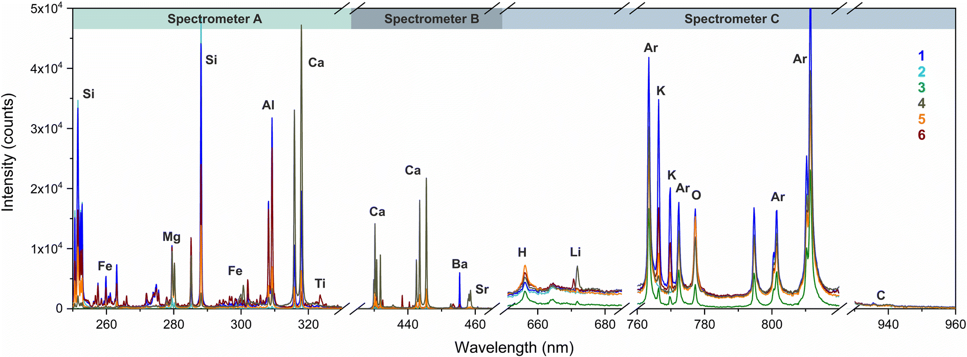Fig. 3 Example of single shot spectra obtained in the M1 sample for 6 component categories: (1) aluminosilicate; (2) quartz; (3) charcoal; (4) carbonate; (5) binder; and (6) tile.

2.4 Learning and validation methodology

Among the 1353 reference spectra associated with the 8 categories, 75% were used for training (i.e., 1018) and 25% for validation (i.e., 335). This spectra selection was done randomly. The validation step consisted in assessing the ANN predictions of known spectra but which were not seen by the ANN during the learning phase. This allows us to evaluate the performance of the network under “real” conditions and to avoid overtraining. The used network was then constituted by 27 neurons in the input layer (associated with the LIBS intensities at 27 selected wavelengths), and 8 neurons in the output layer (associated with the sample categories). The number of neurons in the hidden layer is considered as a parameter to be optimized and it will be discussed in the next section.

The general methodology of data manipulation is presented in Fig. 4, which schematically describes the processing of 6 spectra associated with 6 different categories among the 8 (named from 1 to 6). A pre-treatment, consisting in a normalization, was first applied to each spectrum. This step appeared necessary since all the data presented hereafter were obtained on a rather long time scale. The reference spectra were measured over a few days of experimentation but the imaging data of the three shown samples (M1, M2 and M3) were obtained over a little more than a year. We have evaluated two normalization approaches applied to each of the 3 spectrometers: a normalization by the total intensity of each spectrum and a standard normal variate (SNV) normalization. The results of such normalization will be discussed below. Then, the next step was to extract the selected line intensities. We used the methodology introduced in Motto-Ros et al. (2019),³⁹ which consists in the peak area determination from which the spectral background is subtracted. Before being presented to the ANN (either for the learning or prediction), we decided to rescale all these 27 intensities by the maximum value obtained on all the 1353 reference spectra. This allowed us to compensate the large dynamic range that was observed between certain lines and to provide input values to the ANN between 0 and 1, favoring the network operation. Note that these 27 rescaling factors were obtained from all the set of reference spectra, and then applied to any new incoming spectra. All the software tools used were custom-made and developed in a LabVIEW environment. The computer used for all the processing was a laptop with an Intel i9 processor and 32 GB of RAM. With this computer, the time required for all the processing step of one spectrum was about 180 μs, showing the possibility of implementing it on a LIBS imaging system up to kHz acquisition rate.

Fig. 4 Schematic view of the data manipulation from raw spectra to the final ANN predictions. An indicative temporal strip is given for the treatment of one spectrum.

3. Results

3.1 ANN optimization

As mentioned above, an important step of this work consisted in optimizing the different parameters of the network with the idea to get the best ANN performance. For that we have assessed the MSE (mean square error), giving the average squared difference between the estimated predictions and the reference values. The evaluation of the MSE was done both for the training and the validation datasets. The training MSE can only decrease with the multiplication of iterations, in contrast to the validation MSE that may even show an increase in the presence of overtraining (i.e., the ANN gets too specialized on the exact training set details). These trends are illustrated in Fig. 5a for an ANN trained with 1500 iterations. Here, we have considered as parameters to be optimized: the iteration number of the training algorithm, the type of normalization applied to the spectral data, and the neuron number in the hidden layer. All settings except the studied one were fixed. These trainings were performed five times with the same configuration, from which we have extracted the mean values and the standard deviation (STDV), the latter being used as the error bars in all the graphs shown in Fig. 5. We may note that a typical training (about 1000 iterations) required less than 3 minutes with this computing capability.

Fig. 5 Optimization of ANN parameters with MSE minimization. (a) Example of training with the training and validation MSE curves; (b) optimization of the number of hidden layer neurons; (c) optimization of the number of iterations; (d) evaluation of different types of normalization.

Regarding the number of neurons in the hidden layer (c.f.Fig. 5b), after 45 neurons, the validation MSE ceased to decrease. Considering this value, MSE was then evaluated to search for the optimal iteration number of the learning algorithm. As can be seen in Fig. 5c, validation MSE is optimal for thousands of iterations. This observation was supported by the evolution of the MSE (c.f.Fig. 5a) which shows good stability for the validation set after 800 iterations. Finally, the ANN was tested considering different spectral normalizations: by the sum of the intensities; by the standard normal variate (SNV) which consists in subtracting each spectrum by its own mean and dividing it by its own standard deviation; or without any normalization. Results are shown in Fig. 5d for 45 neurons in the hidden layer. As can be seen, there are no important differences between these three methods even if the sum normalization gives a better performance. To resume, the optimal parameters retained for our ANN were: 45 neurons in the hidden layer, 1000 iterations and a normalization by the sum of the intensities for each spectrum.

Generally speaking, we can observe that there is no significant evolution of the predictive performances according to the network parameters and normalization methods (c.f.Fig. 5). This is a rather positive point because it shows that the network can easily identify the different categories, despite the fact that some of them are very similar. We can also point out the importance of using a validation set (not used during the training) to characterize the performance of the network. We can notice in Fig. 5a–c that the MSE, evaluated on the training set, only decreases when we increase the iteration number or the neuron number in the hidden layer, which is characteristic of overtraining.

In order to implement, in the long term, this type of processing in real time, it was necessary to find a fast and robust way to assign a spectrum to a category. Two examples of predictions related to the validation set are illustrated in Fig. 6a and b. In the first case (i.e., spectrum #724), the prediction is clear and refers to the 5-binder category. In the second case (i.e., spectrum #1215), the situation is more delicate since two categories may be considered: 5-tile and/or 8-aluminoscilicate. The chosen alternative was to introduce a threshold parameter. If the ANN prediction of the category X is higher than the threshold, then the spectrum is identified as having originated from this class. On the other hand, if the prediction value is lower, then the spectrum is classified as coming from an unknown material (i.e., classified as not identified). Note that a sigmoid transfer function is rather insensitive for values close to 0 and 1 (horizontal asymptotes). Therefore, the input values (originally either 0 or 1) were first contracted between 0.05 and 0.95, then a reverse stretch was applied following the prediction. With this necessary contraction and stretch steps, the network can provide negative values and/or values above 1 (c.f.Fig. 6a and b).

Fig. 6 Example of ANN predictions for certain (a) or double-identification spectra (b), and percentage of identification according to different thresholds for (c) all categories, (d) binder, (e) aluminosilicate.

In micro-LIBS imaging, we can also expect to have a certain number of pixels associated with 2 or more categories. This will be the case for all pixels of the image obtained at the interface between 2 (or more) phases. In this case, the inputs will correspond to linear combinations of the reference spectra, and the network will behave as in the example of Fig. 6b by giving an important weight to 2 (or more) categories. Therefore, the definition of the threshold will be an important parameter and adjustable according to the needs of the application. Higher the threshold value, more robust the algorithm will be, i.e., more accurate the identifications will be, but on the other hand, greater the number of unidentified spectra will be. To assess the influence of this threshold, we evaluated the percentage of correct, false, and unidentified assignment obtained on the validation set for each category as well as for the whole. Fig. 6c illustrates the case for all categories. As can be seen, for a threshold of 0, we obtain ∼98% of correct identification and ∼2% of wrong identification (i.e., 6 spectra out of 335). Increasing the threshold value reduces the number of false identifications, thus improving the robustness of the algorithm, but also increases the number of unidentified spectra (prediction below the threshold). It was also important to look at the binder category since our primary objective was to discriminate as accurately as possible the two forms of carbonates present in these samples (geo and neo formed). The results are illustrated in Fig. 6d, which shows excellent prediction capabilities for the binder class. Thereafter, we chose to use a threshold at 0.65 which corresponds, in our point of view, to a good compromise with regard to these results. At this point, it is interesting to note that the 2% of incorrect spectra are mostly associated with the classes: tile, quartz, and aluminosilicate. As shown in Fig. 6e, the percentage of correct identification for aluminosilicate is only in the range of 93%. This is explained by the fact that it is not easy to generate reference spectra of the tile class. These materials have indeed an important number of inclusions of small quartz or silicate aggregates, difficult to discriminate from an elemental point of view, because these 3 types of materials are quite close in terms of composition. For instance, the spectrum shown in Fig. 6b is probably a mixture of both tile and aluminosilicate.

3.2 Archaeological mortar

The first step to test the performance of the network was to apply it on the data collected from the sample M1. These data correspond to a sequence of 900 × 800 pixels obtained with a spatial resolution of 25 μm. The elemental images associated with the 27 selected lines are illustrated in ESI Fig. 1.† As can be seen in this figure, this sample is highly heterogeneous and complex from an elemental point of view. Each of the 720 000 spectra was presented to the network following the same pre-processing and extraction steps (see Fig. 4) as in the training phase. The optical imaging and ANN results are shown in Fig. 7. The time required to process all the data was less than 2 minutes. The colors associated with the different classes have been chosen to best match the natural colors of these materials: beige for the binder, brown for carbonate, blue for quartz, light blue for silicate, green for coal, red for the tile, and gray for the hole.

Fig. 7 Results provided by the ANN obtained on sample M1: (a) optical image of the sample surface. (b) ANN images of the seven detected categories (threshold value of 0.65). (c) ×2.5 zoom of the blue rectangle shown in (b) with various threshold values: 0.25, 0.65 and 0.90. The black pixels in (b) and (c) correspond to unidentified spectra.

As can be seen, the results provided by the ANN show overall an excellent similarity to the optical image (c.f.Fig. 7a and b). These results, as well as the results obtained for samples M2 and M3 (see thereafter), were inspected with great care by our archaeologist colleagues, specialists in these materials, to finally test the network performance in real operation mode. They have indeed reviewed all the minerals (including aggregates, tiles, binders, etc.) generated by the ANN and checked their equivalence to the ones on the samples. Except for a few small minerals, unknown to the network since they were not yet considered in the training set (c.f. below), their conclusions were extremely positive about the network's ability to provide accurate mineral phase identification, and this despite the great complexity and heterogeneity of its materials.

As shown in Fig. 7, the ANN identifies numerous and varied sizes of tile pieces. The tiles used are often of architectural type. The tile itself is a complex material which results from the 900 °C firing of natural clay minerals. These natural clay materials originally contain clay minerals but also some macroscopic minerals: quartz, feldspars and rock fragments. Sometimes, the craftsman may choose to add more sand or clay materials to adapt the ceramic paste properties. The proportions vary according to the potter workshop but also according to the craftsman. There are also practices that consist in washing the clay materials to eliminate the coarsest parts. This is why on the ANN images, within the tile aggregates, we can observe quartz, silicates and carbonates. The presence of aluminum oxides (Al₂O₃), silicon oxides (SiO₂) and iron oxides (Fe₂O₃) in the clay minerals used to make the tiles induces hydraulic properties favorable to their use for the construction and water tightness of aqueducts. This is known as artificial pozzolan. However, the primary quality of these materials was better mechanical resistance, as well as higher durability.⁴⁰ In general, to increase the hydraulic properties, the tile fragments were reduced in size, which led to an increase in the specific contact surface between the lime and the pozzolans. We can also observe on the image of sample M1, 2 layers of mortar with different aggregate sizes. The ANN image also allows us to identify coal. Its sporadic presence would rather suggest a stochastic event. To conclude about this last point, we need to analyze a larger surface area. However, the black aggregate present on the tile in the upper left of the optical image Fig. 7a has been identified by the ANN as a tile. Referring to the elemental images (Fig. 1 ESI†), we notice a relatively high intensity of manganese and oxygen. We can therefore assume that it is a manganese oxide grain in its mineral phase. As the oxides were not entered as input values in the ANN, they will not be identified.

In Fig. 7c, 2 areas (denoted (i) and (ii)) have been identified by the ANN as carbonates, which it distinguishes very well from the binder, although the molecular composition is similar (CaCO₃). This identification is essential because if we plan to carbon 14-date the building, only the carbon of the binder is of interest. Indeed, if we compare with the optical image, (i) could be due to a secondary calcite phase.⁴¹ Secondary calcite corresponds to the formation of new crystals after the mortar has set. In fact, in the presence of ambient water (due to precipitation, surface water and groundwater), the mortar binder could dissolve, react with fresh atmospheric CO₂ and redeposit. Secondary calcite then has a ¹⁴C age younger than the time of construction.⁴² On the other hand, (ii) would appear to correspond to a geological carbonate aggregate. Its ¹⁴C dating would be much earlier than the time of construction. In addition, the influence of the above-described threshold can be observed in Fig. 7c which shows 3 zoomed images obtained with threshold values of 0.25, 0.65 and 0.9. With values close to 1, more spectra are undefined (black pixels). It is important to note that this threshold influences especially spectra registered on interface zones, between different materials, many of which are black with 0.90 threshold for example. It may be attributed to the plurality of contributions in such zones.

The binder, secondary calcite and geological carbonates have very different densities. The binder is porous whereas the geological carbonates are dense. These characteristics have made it possible to discriminate between these different “CaCO₃” type compounds. First of all, as the binder is much more porous, moisture is fixed by physisorption. The hydrogen line is therefore discriminating. Secondly, the “matrix effect” permits the discrimination. The proportion of the intensities of the ionic and atomic Ca lines (Ca II and Ca I) differs according to the nature of the calcium carbonates. Various parameters influence the plasma composition and thus the intensity of the lines, in particular the ablated mass, the electronic temperature and the electronic density. At thermal equilibrium, the physical behavior within the plasma is governed by the Boltzmann equation and the Saha equation.⁴³ It is found that the plasma temperature (between 7000 and 12 000 K) and the amount of material depend on the ablated material, in particular its melting temperature and density. Indeed, denser the material, higher the plasma temperature, which is the case for geological carbonate that is denser than the porous binder. Furthermore, a hotter plasma favors the ionization of species, which is in agreement with the higher intensities of calcium ion lines for denser carbonates (whose plasma is therefore hotter). Conversely, the binder shows high Ca I line intensities, which can be explained by a colder plasma in this porous phase. Thus, variations in the plasma properties for materials of the same chemical composition induce variations specific to each emission line, which then allow these differences to be observed. The influence of the atomic H I (656.10 nm), Ca I (318.13 nm and 643.91 nm) and ionic Ca II (458.52 nm) lines has been evaluated with a quaternary diagram (Fig. 2 ESI†). Note that the secondary crystallizations seem close to the geological phase but intermediate with the micritic crystallization of the binder.

The same treatment was then applied to two other datasets (samples M2 and M3). These samples have been characterized in great detail in a previous article.²⁴ Our objective was to evaluate the robustness of the methodology on an extended measurement period. Indeed, the LIBS measurements in M1 are about one year behind those in M2 and M3. Besides, during this time, the micro-LIBS instrument moved to another building and had to be totally reconfigured and optimized. M2 and M3 also differ in their preparation. M2 and M3 were embedded in resin but M1 was measured raw. The comparison of results in Fig. 7 and 8 shows the robustness of the ANN. In M2 and M3, we notice that unlike M1, there is no charcoal. M2, like M1, contains tiles, probably due to its hydraulic properties. M3, on the other hand, does not contain tiles but aggregates of quartz, silicate, and carbonate which could correspond to sand. In Richiero et al.,²⁴ the sand origin from the Maine River, which flows at the foot of the cathedral, was assumed due to the different natures of the silicates. At present, the ANN does not allow classification of the different silicates.

Fig. 8 Results provided by the ANN obtained on sample M2 and M3. Both samples were embedded in epoxy resin. (a) Optical image of the sample M2. (b) ANN images of M2 for the seven detected categories (threshold value of 0.65). (c) Optical image of M3. (d) ANN images of M3 for the detected categories (threshold value of 0.65). Note that the charcoal category is not displayed since it was not detected in both samples.

4. Discussion

The proposed methodology is based on the use of a relatively simple ANN (only 80 neurons) yet very efficient in terms of robustness, prediction quality and response time (<ms per spectrum). It allows us to consider this type of processing directly during the experiment in order to have an almost real time processing of the spectra and the display of the image as the experiment progresses. This could indeed be of great interest for industrial applications and for simplified routine analyses. For our case study (i.e., characterization of archaeological mortars), this processing method addresses several important obstacles. First of all, we have shown no difficulties in identifying the different forms of carbonates (in particular geo-formed aggregates and binder) which opens up good prospects for their use in the framework of carbon-14 dating. Then, the identification of mineral phases and the generation of masks is now automatic and no longer requires the intervention of human supervision to set the threshold, often arbitrarily, as was the case in our previous article.²⁴ The global characterization of the samples (not shown here), including the evaluation of the different proportions between the binder/tile/aggregates/or others, the size and the shape of the aggregates now becomes fast and undoubtedly more accurate.

One point that must be emphasized is the importance of the reference spectra. The more the base of spectra used for the learning is rich and well mastered, the more the network will be efficient, both in its training and its predictions. Here we have chosen to create a general category representing all the aluminosilicates. However, this class of material is much broader than those considered in this study. We will have to acquire a greater number of known minerals and expand this category. One advantage of the use of neural networks is that it is possible to apply several networks in cascade, and we could for example add a second network, which will treat specifically the class of aluminosilicates.

It is true that an ANN will identify known signatures and will obviously be unable to identify unknown materials. However, it can be interesting to observe the global set of predictions of the ANN. An example is given in Fig. 9 where we represent the sum of all the predictions provided by the network for the sample M3. For an optimal behavior of the network obtained on a known material, we expect to obtain one output neuron close to 1 and the other outputs close to 0. Under normal conditions, the sum should thus be around 1, which is represented by the grey regions of Fig. 9. On the other hand, for unknown spectra (i.e., materials absent from the training), two possibilities exist. First, in the case where the spectral structure is totally different from the training set, one can expect to obtain a low prediction for all output neurons. This will result in a sum much lower than 1. Such a case is, a priori, not observed in the case of sample M3. Second, the most likely case is that a spectrum contains information associated with several classes. In this case, the sum of the output neurons will be higher than 1 (red to yellow color in Fig. 9). This may occur mainly for measurements taken at the interface between two mineral phases, but the arrow indicated by (i) in Fig. 9b shows a small aggregate not detected so far containing both Ca and Si as major elements, as illustrated in the spectrum of Fig. 9c. Such types of materials, containing Ca and Si as major elements, were not taken into account during learning. Such a type of representation can be very interesting to identify spectra out of categories, and thus reveal exotic spectra. In addition, this can also be used to define an additional confidence level for the inclusion or exclusion of the pixels concerned.

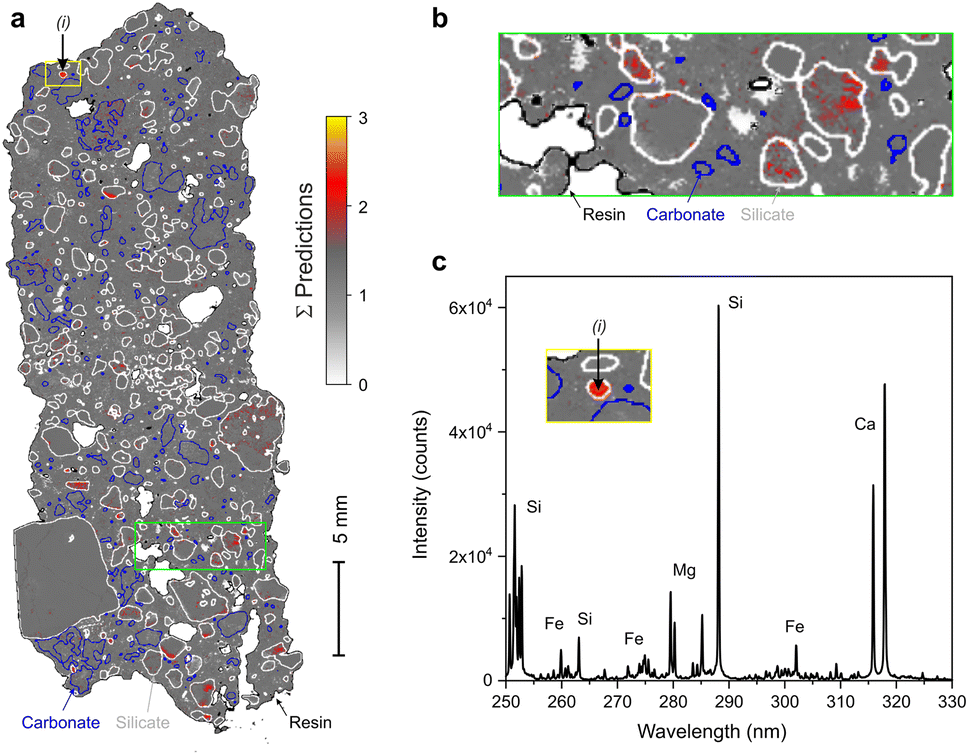Fig. 9 (a) Sum of all the predictions for sample M3. (b) Zoom on the region indicated by a green rectangle in (a). (c) Single shot spectrum corresponding to a pixel of the red spot (i) observed in (b).

5. Conclusion

In this paper, we have demonstrated that the use of an ANN algorithm for the processing of LIBS imaging data may be helpful as much as powerful. Even a simple network structure, a 3-layer perceptron with 80 neurons in total, can provide a fast, automated, robust, and efficient processing for a large number of spectra. Its optimization points out that the ANN robustness does not depend so much on its own parameters (neuron number in the hidden layer, iteration number for the training, and spectra normalization) as on the quality of the reference dataset for training. The accuracy of the final identification is also improved by the use of a threshold on output values, to allow as much identifications as possible and avoiding misrecognition.

In particular, for mortar characterization, ANN provides good identification of spectra thanks to a specific training on nearly 1000 spectra which has been validated on a 300 spectra set. It allows us to supply in an automatic way a mask of each mineral phase present on the mortar surface, depending on the component categories we implemented. Furthermore, it clearly differentiates the calcium carbonates from the binder and from other origins (geological especially and secondary phase probably) that may be due to the difference in the densities of each one (quantity ablated and plasma parameters), as well as the physisorption of H₂O in the binder (micro)porosity. It allows us to precisely map the mortar and determine where the lime binder of interest for radiocarbon dating is.

Nevertheless, ANN treatment is limited by the training dataset; to improve its capacity of mineral identification, it will be necessary to implement more data and a broader reference dataset in terms of their mineralogical nature. The use of different interlinked neural networks would also be useful for the specific identification of some minerals, such as silicates. Thus, it could be then translated to the analysis of other geological or composite materials, such as archaeological ceramics, but also to any sample kind in general. In the future, experimental data could be implemented in an ANN in real time, spectrum by spectrum, for a synchronous treatment with the acquisition. This would provide robust compound identification results immediately following LIBS measurements.

Author contributions

The final manuscript was written through contributions of all authors.

Conflicts of interest

The authors declare that they have no known competing financial interests or personal relationships that could have appeared to influence the work reported in this paper.

Acknowledgements

This work was partially supported by the French region Rhônes Alpes Auvergne (Optolyse, CPER2016), the French “Agence Nationale de la Recherche” (ANR-22-xxx “MEMOAr” and ANR-20-CE17-0021 “dIAg-EM), and the French government “France 2030” initiative, under the DIADEM program managed by the “Agence Nationale de la Recherche” (ANR-22-PEXD-0014, “Libelul”). This project has also received financial support from the CNRS through the MITI interdisciplinary programs ("CaPhyMOAr"). In addition, we gratefully acknowledge Dr Frédéric Pelascini from the Cétim Grand Est and Dr Florian Trichard from Ablatom, for fruitful discussions.

Notes and references

1. A. Limbeck, L. Brunnbauer, H. Lohninger, P. Pořízka, P. Modlitbová, J. Kaiser, P. Janovszky, A. Kéri and G. Galbács, Anal. Chim. Acta, 2021, 1147, 72–98,  DOI:10.1016/j.aca.2020.12.054.
2. L. Jolivet, M. Leprince, S. Moncayo, L. Sorbier, C.-P. Lienemann and V. Motto-Ros, Spectrochim. Acta, Part B, 2019, 151, 41–53,  DOI:10.1016/j.sab.2018.11.008.
3. B. Busser, S. Moncayo, J.-L. Coll, L. Sancey and V. Motto-Ros, Coord. Chem. Rev., 2018, 358, 70–79,  DOI:10.1016/j.ccr.2017.12.006.
4. C. Fabre, D. Devismes, S. Moncayo, F. Pelascini, F. Trichard, A. Lecomte, B. Bousquet, J. Cauzid and V. Motto-Ros, J. Anal. At. Spectrom., 2018, 33, 1345–1353,  10.1039/C8JA00048D.
5. J. O. Cáceres, F. Pelascini, V. Motto-Ros, S. Moncayo, F. Trichard, G. Panczer, A. Marín-Roldán, J. A. Cruz, I. Coronado and J. Martín-Chivelet, Sci. Rep., 2017, 7, 5080,  DOI:10.1038/s41598-017-05437-3.
6. B. Busser, A. Bulin, V. Gardette, H. Elleaume, F. Pelascini, A. Bouron, V. Motto-Ros and L. Sancey, J. Neurosci. Methods, 2022, 379, 109676,  DOI:10.1016/j.jneumeth.2022.109676.
7. A. Cugerone, B. Cenki-Tok, M. Muñoz, K. Kouzmanov, E. Oliot, V. Motto-Ros and E. Le Goff, Miner. Deposita, 2021, 56, 685–705,  DOI:10.1007/s00126-020-01000-9.
8. F. Trichard, F. Gaulier, J. Barbier, D. Espinat, B. Guichard, C.-P. Lienemann, L. Sorbier, P. Levitz and V. Motto-Ros, J. Catal., 2018, 363, 183–190,  DOI:10.1016/j.jcat.2018.04.013.
9. B. Busser, S. Moncayo, F. Trichard, V. Bonneterre, N. Pinel, F. Pelascini, P. Dugourd, J.-L. Coll, M. D'Incan, J. Charles, V. Motto-Ros and L. Sancey, Mod. Pathol., 2018, 31, 378–384,  DOI:10.1038/modpathol.2017.152.
10. S. Moncayo, L. Duponchel, N. Mousavipak, G. Panczer, F. Trichard, B. Bousquet, F. Pelascini and V. Motto-Ros, J. Anal. At. Spectrom., 2018, 33, 210–220,  10.1039/c7ja00398f.
11. P. Pořízka, J. Klus, E. Képeš, D. Prochazka, D. W. Hahn and J. Kaiser, Spectrochim. Acta, Part B, 2018, 148, 65–82,  DOI:10.1016/j.sab.2018.05.030.
12. A. Nardecchia, C. Fabre, J. Cauzid, F. Pelascini, V. Motto-Ros and L. Duponchel, Anal. Chim. Acta, 2020, 1114, 66–73,  DOI:10.1016/j.aca.2020.04.005.
13. A. Nardecchia, A. de Juan, V. Motto-Ros, M. Gaft and L. Duponchel, Anal. Chim. Acta, 2022, 1192, 339368,  DOI:10.1016/j.aca.2021.339368.
14. Q. Wu, C. Marina-Montes, J. Caceres, J. Anzano, V. Motto-Ros and L. Duponchel, Spectrochim. Acta, Part B, 2022, 195, 106508,  DOI:10.1016/j.sab.2022.106508.
15. J. Sirven, B. Bousquet, L. Canioni, L. Sarger, S. Tellier, M. Potin-Gautier and I. Le Hecho, Anal. Bioanal. Chem., 2006, 385, 256–262,  DOI:10.1007/s00216-006-0322-8.
16. M. Stepputat and R. Noll, Appl. Opt., 2003, 42, 6210–6220,  DOI:10.1364/AO.42.006210.
17. K. Wei, Q. Wang, G. Teng, X. Xu, Z. Zhao and G. Chen, Appl. Sci., 2022, 12, 4981,  DOI:10.3390/app12104981.
18. W. Xu, C. Sun, Y. Zhang, Z. Yue, S. Shabbir, L. Zou, F. Chen, L. Wang and J. Yu, J. Anal. At. Spectrom., 2022, 37, 317–329,  10.1039/D1JA00366F.
19. A. Coutelas, Éditions Errance, Le mortier de chaux, Paris (France), 2009.
20. R. Hayen, M. Van Strydonck, L. Fontaine, M. Boudin, A. Lindroos, J. Heinemeier, Å. Ringbom, D. Michalska, I. Hajdas, S. Hueglin, F. Marzaioli, F. Terrasi, I. Passariello, M. Capano, F. Maspero, L. Panzeri, A. Galli, G. Artioli, A. Addis, M. Secco, E. Boaretto, C. Moreau, P. Guibert, P. Urbanova, J. Czernik, T. Goslar and M. Caroselli, Radiocarbon, 2017, 59, 1859–1871,  DOI:10.1017/RDC.2017.129.
21. P. Urbanová, E. Boaretto and G. Artioli, Radiocarbon, 2020, 62, 503–525,  DOI:10.1017/RDC.2020.43.
22. S. Pagnotta, M. Lezzerini, L. Ripoll-Seguer, M. Hidalgo, E. Grifoni, S. Legnaioli, G. Lorenzetti, F. Poggialini and V. Palleschi, Appl. Spectrosc., 2017, 71, 721–727,  DOI:10.1177/0003702817695289.
23. S. Živković, A. Botto, B. Campanella, M. Lezzerini, M. Momčilović, S. Pagnotta, V. Palleschi, F. Poggialini and S. Legnaioli, Spectrochim. Acta, Part B, 2021, 181, 106219,  DOI:10.1016/j.sab.2021.106219.
24. S. Richiero, C. Sandoval, C. Oberlin, A. Schmitt, J.-C. Lefevre, A. Bensalah-Ledoux, D. Prigent, C. Coquidé, A. Valois, F. Giletti, F. Pelascini, L. Duponchel, P. Dugourd, C. Comby-Zerbino and V. Motto-Ros, Appl. Spectrosc., 2022, 1–10,  DOI:10.1177/00037028211071141.
25. J. El Haddad, L. Canioni and B. Bousquet, Spectrochim. Acta, Part B, 2014, 101, 171–182,  DOI:10.1016/j.sab.2014.08.039.
26. E. C. Ferreira, D. M. B. P. Milori, E. J. Ferreira, R. M. Da Silva and L. Martin-Neto, Spectrochim. Acta, Part B, 2008, 63, 1216–1220,  DOI:10.1016/j.sab.2008.08.016.
27. Y. Zhao, M. L. Guindo, X. Xu, M. Sun, J. Peng, F. Liu and Y. He, Appl. Spectrosc., 2019, 73, 565–573,  DOI:10.1364/AS.73.000565.
28. T. Chen, L. Sun, H. Yu, W. Wang, L. Qi, P. Zhang and P. Zeng, Appl. Geochem., 2022, 136, 105135,  DOI:10.1016/j.apgeochem.2021.105135.
29. F. Henrion, Bull. Monum., 2001, 159, 77–89,  DOI:10.3406/bulmo.2001.970.
30. A. Coutelas, Aquitania, 2012, 28, 171–178,  DOI:10.3406/acquit.2012.977.
31. S. Büttner, in Chantiers et matériaux de construction : De l'Antiquité à la Révolution industrielle en Orient et en Occident, ed. A. Baud and G. Charpentier, Lyon, 2020.
32. A. Coutelas, G. Godard, P. Blanc and A. Person, Rev. Archéom., 2004, 28, 127–139,  DOI:10.3406/arsci.2004.1068.
33. A. Moropoulou, K. Bisbikou and A. Bakolas, J. Cult. Herit., 2000, 1, 45–58,  DOI:10.1016/S1296-2074(99)00118-1.
34. A. Borlenghi and A. Schmitt, SRA Auvergne Rhône-Alpes, Aqueduc du Gier, étude du pont-siphon de Beaunant et relevé de la partie terminale du tracé de l’aqueduc. Rapport de prospection thématique, 2018.
35. C. Coquidé and G. Macabéo, Rev. Archeol. de l'Est, 2010, 59, 447–504.
36. A. Borlenghi and C. Coquidé, Dossier : Les aqueducs romains de Lyon, nouvelles approches sur un cas d’étude unique, Gallia, 2023 , in press.
37. C. Coquidé and A. Valois, Dossier : Les aqueducs romains de Lyon, nouvelles approches sur un cas d’étude unique, Gallia, 2023 , in press.
38. D. Prigent, in Anjou: Medieval Art, Architecture, and Archaeology, ed. J. Mcneil and D. Prigent, 2003, pp. 14–33.
39. V. Motto-Ros, S. Moncayo, F. Trichard and F. Pelascini, Spectrochim. Acta, Part B, 2019, 155, 127–133,  DOI:10.1016/j.sab.2019.04.004.
40. A. Coutelas, in Mortiers et hydraulique en Méditerranée antique, 2019.
41. T. S. Daugbjerg, A. Lindroos, J. Heinemeier, Å. Ringbom, G. Barrett, D. Michalska, I. Hajdas, R. Raja and J. Olsen, Archaeometry, 2021, 63, 1121–1140,  DOI:10.1111/arcm.12648.
42. G. Macleod, A. E. Fallick and A. J. Hall, Chem. Geol. Isot. Geosci., 1991, 86, 335–343,  DOI:10.1016/0168-9622(91)90015-O.
43. A. De Giacomo and J. Hermann, J. Appl. Phys., 2017, 50, 183002,  DOI:10.1088/1361-6463/aa6585.

---

Footnote

† Electronic supplementary information (ESI) available. See DOI: https://doi.org/10.1039/d2ja00389a

---