 Open Access Article
 This Open Access Article is licensed under a Creative Commons Attribution-Non Commercial 3.0 Unported Licence
Hunting for interstellar molecules: rotational spectra of reactive species†
Cristina
Puzzarini
 *,
Silvia
Alessandrini
,
Luca
Bizzocchi
* and
Mattia
Melosso
*
*,
Silvia
Alessandrini
,
Luca
Bizzocchi
* and
Mattia
Melosso
*
ROT&Comp Lab, Department of Chemistry “Giacomo Ciamician”, University of Bologna, Via F. Selmi 2, I-40126 Bologna, Italy. E-mail: cristina.puzzarini@unibo.it; luca.bizzocchi@unibo.it; mattia.melosso2@unibo.it
First published on 14th March 2023
Abstract
Interstellar molecules are often highly reactive species, which are unstable under terrestrial conditions, such as radicals, ions and unsaturated carbon chains. Their detection in space is usually based on the astronomical observation of their rotational fingerprints. However, laboratory investigations have to face the issue of efficiently producing these molecules and preserving them during rotational spectroscopy measurements. A general approach for producing and investigating unstable/reactive species is presented by means of selected case-study molecules. The overall strategy starts from quantum-chemical calculations that aim at obtaining accurate predictions of the missing spectroscopic information required to guide spectral analysis and assignment. Rotational spectra of these species are then recorded by exploiting the approach mentioned above, and their subsequent analysis leads to accurate spectroscopic parameters. These are then used for setting up accurate line catalogs for astronomical searches.
1 Introduction
Since the discovery of the first polyatomic molecules in the late 1960s and early 1970s, it soon became clear that the interstellar medium (ISM) is characterized by a rich chemistry. Because of the extreme conditions of the ISM, with temperatures ranging between 10 and 100 K, very low densities (from 10 to 108 molecules cm−3), and ionizing radiation, the chemistry there occurring leads to the formation of exotic molecules.1–4 Among the about 270 molecules detected in the ISM and circumstellar shells so far, a sizeable number of them are species that under terrestrial conditions are unstable and/or highly reactive.5 The list includes radicals and ions, but also closed-shell unsaturated systems such as imines and carbon chains. Illustrative examples are the HC5O radical,6,7 the C8H− negative ion,8,9 the HC9N carbon chain,10 the protonated HC5NH+ carbon chain,11 substituted imines like allylimine,12 and the unstable enol form of glycolaldehyde, i.e. (Z)-1,2-ethenediol enol.13 These examples give an idea of the exotic chemistry taking place in the ISM and provide a clear evidence of the fact that unstable and/or reactive species are produced and survive long enough to be detected. In parallel, this chemistry also leads to small organic molecules (denoted as “interstellar” complex organic molecules, COMs14) such as N-methylformamide (CH3NHCHO),15 urea (NH2C(O)NH2),16,17 ethanolamine (HOCH2CH2NH2),18 and n-propanol (CH3CH2CH2OH).19,20Molecular spectroscopy plays a central role in the discovery of interstellar molecules,5,21 with the overwhelming majority of chemical species in the cosmos being discovered via their rotational signatures. Indeed, the astronomical observation of the rotational spectroscopic features of a given molecule provides unequivocal proof of its presence in the astronomical environment under consideration.5,21–23 In principle, the systematic observation of a given astronomical source leads to a complete census of its molecular content. However, astronomical line surveys still reveal unknown features, the main reason being the lack of corresponding spectroscopic information.5,21 As suggested above, interstellar species can be short-lived systems on Earth, this rendering their spectroscopic characterization a challenging task. Indeed, molecular species that are not yet studied in the laboratory show relevant difficulties in their production. This is the topic touched on in this work. Radicals and ions are transient species which are typically generated in situ using plasma techniques.24–26 Neutral, closed-shell unsaturated species such as carbon chains are stable molecules that, however, tend to be highly reactive and thus need to be produced in situ as well.
In this contribution, a laboratory strategy pursued to obtain very accurate line catalogs for guiding the astronomical search of unstable and/or reactive species is presented. Illustrative systems that are produced either using flash vacuum pyrolysis27–29 or DC discharge24–26 are investigated. As examples of closed-shell reactive species, the DC7N and ClC3N carbon chains have been studied, while as examples of open-shell systems, the CCS and CH2CN radicals are considered. The strategy relies on the interplay of experiment and theory, which is crucial because it often happens that, for this type of molecular species, no previous experimental data are available and the study starts from an accurate computational characterization.12,28 In the following section (Methods), the strategy is introduced; then, the experimental and computational aspects are detailed. Subsequently, the results for the species mentioned above are presented and discussed. Finally, in the last section, conclusions are drawn.
2 Methods
As mentioned in the Introduction, an accurate spectroscopic characterization is required to guide astronomical observations. The interplay of experiment and theory in the field of rotational spectroscopy to be exploited in astronomical searches is graphically represented in Fig. 1. As shown there, the strategy starts with accurate quantum-chemical computations of the spectroscopic parameters (those of an effective Watson-type Hamiltonian) required for the prediction of the rotational spectrum. The simulated spectrum is used to plan the experiment and, once the experimental counterpart is available, is employed to guide spectral analysis and assignment. The subsequent step is the fitting of the assigned transitions with a suitable effective Hamiltonian (the same used for simulation), with the computed parameters providing the starting point. The fitting procedure eventually leads to the set up of a spectroscopic line catalog, which is then used to search for the molecule in the astronomical line surveys.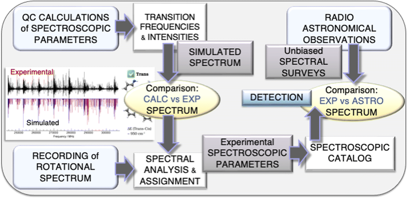 | ||
| Fig. 1 Graphical representation of the interplay of experiment and theory exploited at the ROT&Comp laboratory in Bologna for hunting molecular species in the ISM. | ||
An illustrative example of this strategy at work is provided by ref. 13 and 28: (Z)-1,2-ethenediol, a key prebiotic intermediate in the formose reaction, has been spectroscopically characterized in the laboratory,28 thus providing the line list allowing its detection.13Fig. 2 provides a graphical representation of how the quantum-chemical calculations allowed an easy assignment of the experimental spectrum. In this respect, it has to be noted that no previous spectroscopic information was available for (Z)-1,2-ethenediol, which – being an unstable molecule – was produced by flash vacuum pyrolysis. Another recent example for this strategy at work is provided by ref. 12.
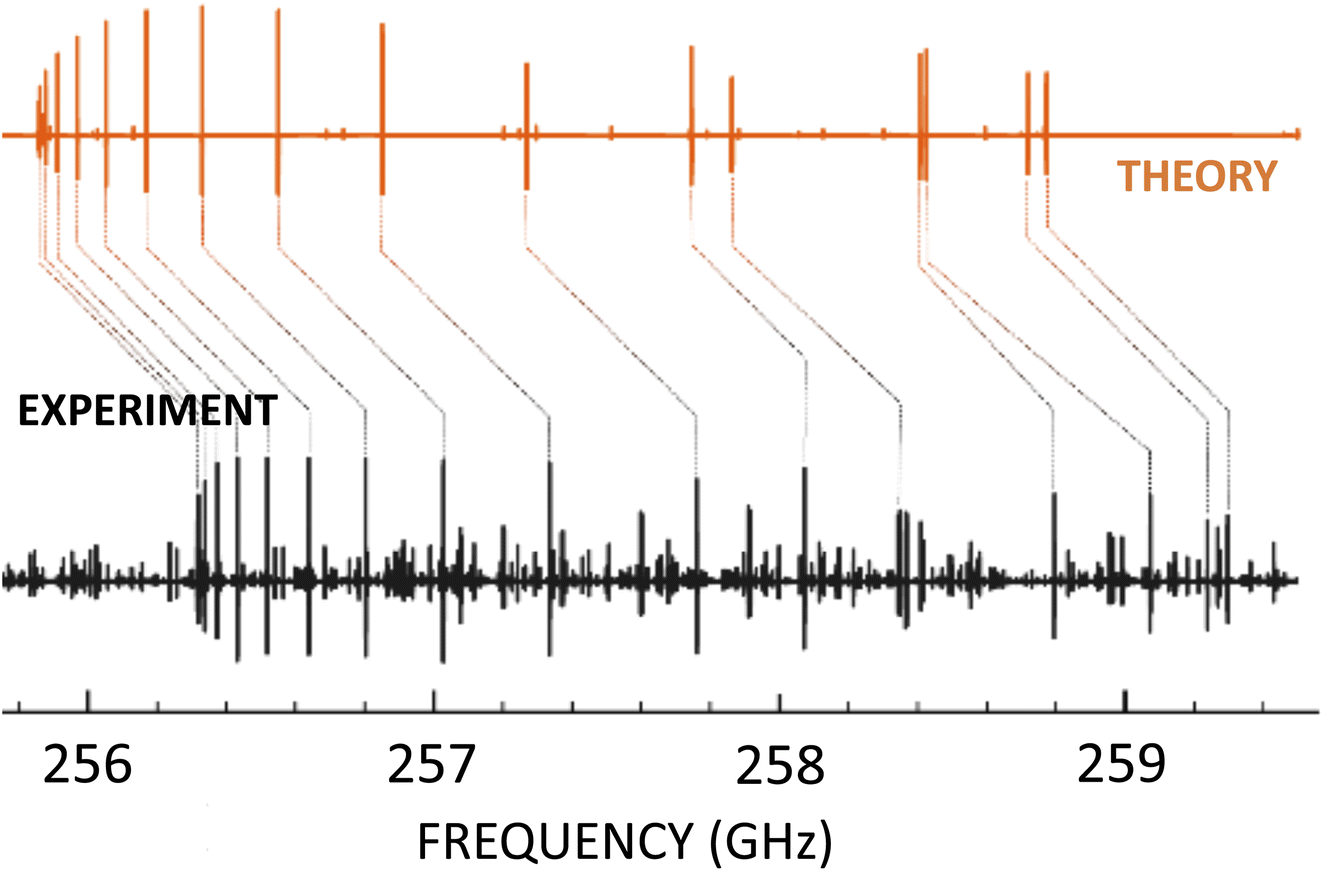 | ||
| Fig. 2 Portion of the millimeter-wave spectrum of (Z)-1,2-ethenediol in the 256–259 GHz range: the experimental spectrum (in black) is compared with the computational simulation (in orange). | ||
In the following section the experimental aspects of the strategy are presented, while in the subsequent one the details of the quantum-chemical calculations are provided. In this work, the focus is on unstable and/or reactive molecules. Therefore, the challenge of the production of these species is mainly addressed.
2.1 Experimental details
The rotational spectrometer employed in this work is a frequency-modulation millimeter/sub-millimeter-wave (mm/sub-mm) spectrometer working in the 75 GHz to 1.6 THz range, which is described in detail in ref. 30 and 31. In short, radiation is produced by a series of Gunn oscillators covering the 75–134 GHz range. Higher frequencies, up to the THz regime, are obtained by means of passive frequency multipliers. Frequency and phase are stabilized by a phase-lock loop. The detection system consists of either Schottky barrier diodes or a liquid-helium-cooled InSb hot electron bolometer (QMC Instr. Ltd type QFI/2). In all cases, the output signal is demodulated by a lock-in amplifier set at twice the modulation frequency, thus leading to second harmonic (2f) detection (nearly second derivative of the line profile). To produce unstable and/or reactive molecules, such as ions, radicals, imines and carbon chains, the mm/sub-mm spectrometer is combined with either a flash vacuum pyrolysis system29 or a DC discharge apparatus.25,26Concerning the flash vacuum pyrolysis (FVP) technique, two different apparatuses can be employed. The first system is constituted by a 30 cm long tubular oven which surrounds a quartz tube directly connected to one inlet of the spectrometer absorption cell. This latter is a glass tube 3.25 m long and 5 cm in diameter. The maximum temperature that can be reached by the oven is 1200 °C. In the second apparatus, a 1.5 m long quartz absorption cell is surrounded by a 90 cm tubular furnace, which is able to reach the same temperature as the first system. Since the cell and oven lengths are different, the heating is inhomogeneously distributed along the cell, with the pyrolysis reaction being confined to the 90 cm directly heated by the oven. To increase the length of the reactive area, a double-pass configuration is arranged,32 with the effective absorption path of the pyrolysis products increasing to, at least, 1.8 m. For both apparatuses, in view of the unstable nature of the target molecules, measurements are performed in dynamic conditions, i.e. a tenuous flow of fresh pyrolysis products is continuously provided by the vacuum system. In all experiments, the production conditions are optimized by adjusting the temperature of the precursor, the temperature of the pyrolysis apparatus, and the pressure of the gaseous products inside the absorption cell.
Moving to the species investigated in this work, ClC3N and DC7N have been produced by means of FVP. Gaseous samples of ClC3N have been produced by co-pyrolysis of carbon tetrachloride (CCl4) and acetonitrile (CH3CN) in a 3![[thin space (1/6-em)]](https://www.rsc.org/images/entities/char_2009.gif) :1 abundance ratio. Typically, 60 mTorr (8 Pa) of CCl4 and 20 mTorr (∼3 Pa) of CH3CN were flowed into the tubular quartz reactor heated at 1150 °C. The measurements were performed while continuously pumping the pyrolysis products through the absorption cell, which was kept at a pressure of ∼5 mTorr (∼1 Pa). ClC3N is moderately stable in the gas phase. Trapping and conservation of the compound at liquid nitrogen temperature is also possible. Purification of the samples via low-temperature distillation has been attempted and proved it was possible to achieve a factor of 2 improvement in the intensity of the absorption signals. DC7N was produced by co-pyrolysis of fully-deuterated toluene (toluene-d8) and trichloroacetonitrile (Cl3CCN) at 1200 °C. The mixture composition was adjusted to have a constant flow of 150 mTorr (20 Pa) of Cl3CCN and 5–10 mTorr (∼1 Pa) of toluene-d8 in the pyrolysis reactor. This corresponds to a pressure of ∼15 mTorr (∼2 Pa) after the expansion of the reaction products in the absorption cell.
:1 abundance ratio. Typically, 60 mTorr (8 Pa) of CCl4 and 20 mTorr (∼3 Pa) of CH3CN were flowed into the tubular quartz reactor heated at 1150 °C. The measurements were performed while continuously pumping the pyrolysis products through the absorption cell, which was kept at a pressure of ∼5 mTorr (∼1 Pa). ClC3N is moderately stable in the gas phase. Trapping and conservation of the compound at liquid nitrogen temperature is also possible. Purification of the samples via low-temperature distillation has been attempted and proved it was possible to achieve a factor of 2 improvement in the intensity of the absorption signals. DC7N was produced by co-pyrolysis of fully-deuterated toluene (toluene-d8) and trichloroacetonitrile (Cl3CCN) at 1200 °C. The mixture composition was adjusted to have a constant flow of 150 mTorr (20 Pa) of Cl3CCN and 5–10 mTorr (∼1 Pa) of toluene-d8 in the pyrolysis reactor. This corresponds to a pressure of ∼15 mTorr (∼2 Pa) after the expansion of the reaction products in the absorption cell.
The mm/sub-mm spectrometer can also be equipped with a negative glow-discharge cell to produce either ionic or radical species. To improve the signal-to-noise ratio (S/N), measurements can be carried out at low temperature (e.g. by circulation of liquid nitrogen in an external plastic pipe tightly wound around the cell). Ions or radicals are prepared directly inside the absorption cell starting from a suitable mixture of gases and by applying a DC discharge of a few mA to some tens of mA. A buffer gas (usually, He or Ar) is often employed together with the precursor(s). Measurements are always performed in a continuous flow of gas, maintained by a diffusion pump, in order to constantly provide fresh precursor gases and remove degraded products. For ions, a longitudinal magnetic field can be applied to improve the S/N. In the case of radicals, this can be used to disentangle their signal from those of the closed-shell species whose transitions contaminate the spectral window. In this work, we considered a sulfur-containing radical, CCS, which has been produced using CS2 as precursor and He as buffer gas in a 2:1 ratio. In most of the measurements, the combination of 30 mTorr (4 Pa) of CS2 with 15 mTorr (2 Pa) of He has been employed, and a DC discharge of 70–75 mA applied.
2.2 Computational details
The pieces of information required for predicting rotational spectra are:• rotational parameters,
• type of transitions observable (and their intensity),
• if relevant, hyperfine parameters.
In Table 1, the correlation between the spectroscopic and molecular parameters to be predicted and the quantities determinable by quantum chemistry is summarized. While in the following the first and third point of the list above are discussed, when considering the type of transitions observable and their intensity, the crucial information is the electric dipole moment or better its components along the inertial axes.33 As pointed out in Table 1, the dipole moment is a first order property which can be obtained from dedicated computations, but also as a byproduct in geometry optimizations.
| Parameter | Symbol(s) | Computational task(s) |
|---|---|---|
| Rotational constants | A e, Be, Ce | Geometry optimization |
| Vibrational corrections to Be values | ΔBvib | Anharmonic force field |
| Quartic centrifugal-distortion constants | D J, DK, DJK, … | Harmonic force field |
| Sextic centrifugal-distortion constants | H J, HK, HJK, … | Anharmonic force field |
| Electric dipole moment | μ | First derivative of electronic energy with respect to electric-field components |
| Nuclear quadrupole coupling constants | χ ij | Electric-field gradient (first derivative of electronic energy with respect to quadrupole moment) |
Rotational parameters include rotational and centrifugal distortion constants. Rotational constants are by far the leading terms and can be seen as formed by two contributions: the dominant one (about 99%) which only depends on the equilibrium structure and the vibrational correction (vide infra) which depends on the coupling between the rotational and vibrational motion.34,35 It is thus clear that accurate equilibrium structures are needed in order to get accurate equilibrium rotational constants.34,36,37 To reach high accuracy, basis-set and electron-correlation effects must be accounted for simultaneously, and this is accomplished by exploiting quantum-chemical composite schemes.38 In these approaches, the various contributions are evaluated separately at the highest possible level and then combined in order to obtain the best theoretical estimate, thereby exploiting the additivity approximation. In the literature, several composite schemes have been proposed in order to obtain the best possible compromise between accuracy and computational cost.37,39–51
In this work, we employed a so-called “gradient scheme” entirely based on coupled-cluster (CC) theory,39,40 which is implemented in the CFOUR quantum-chemistry package.52 In this approach, the additivity approximation is exploited at the energy-gradient level to be minimized for obtaining the equilibrium structure. In particular, we employed the CCSD(T)/CBS+CV scheme, where CCSD(T) stands for the CC singles and doubles (CCSD) approximation augmented by a perturbative treatment of triple excitations.53 The CBS acronym implies the extrapolation to the complete basis set (CBS) limit, while CV refers to the incorporation of the core-valence correlation contribution. The energy gradient to be minimized contains three terms. The first two contributions are the gradients for the separate extrapolation of HF-SCF (Hartree-Fock Self Consistent Field) and CCSD(T) correlation energies to the CBS limit using an exponential extrapolation54 for the former and the n−3 extrapolation scheme55 for the latter. Extrapolation to the CBS limit requires a hierarchy of bases to be employed, with the correlation-consistent valence cc-pVnZ bases56,57 being used in this work, with n = T, Q, 5 for HF-SCF and n = T, Q for CCSD(T). The third term incorporates the CV correlation effects because the CCSD(T) extrapolation to the CBS is performed within the frozen-core (fc) approximation. The CV correction is obtained as the difference of all-electron (ae) and fc CCSD(T) calculations using the same core-valence basis set, which is cc-p(w)CVnZ (n = T, Q) in the present case.58,59
If required by the dimension of the molecule, to obtain accurate equilibrium structures while retaining a feasible computational cost, one can resort to the so-called “cheap-composite” scheme,41,48 which – starting from fc-CCSD(T)/cc-pVTZ calculations – incorporates the extrapolation to the CBS limit and the effect of core correlation at the MP2 level (MP2 stands for second-order Møller–Plesset perturbation theory60). For larger systems for which even the “cheap-composite” scheme becomes too expensive, such as small polycyclic aromatic hydrocarbons (PAH),61 a possible way-out is offered by the so-called “Lego brick” approach.61,62 The idea at its basis is that the system can be seen as formed by different fragments (i.e., the “Lego bricks”), whose accurate equilibrium geometries are available, with the template molecule (TM) approach63 being employed to account for the modifications occurring when moving from the isolated fragment to the molecular system under consideration. To correct the linkage between different fragments, the linear regression (LR) model is then employed.64,65 For the accurate determination of the equilibrium structure of the fragments, in this work, we have resorted to the so-called semi-experimental (SE) approach.63,66,67 The SE equilibrium structural parameters are determined by a linear least-squares fit of the SE equilibrium rotational constants of different isotopologues. These are obtained by correcting the experimental ground-state rotational constants (Bexp0) with computed vibrational (ΔBcalcvib) corrections.66
In the following, we refer to the “Lego brick” approach as TM+LR, or only TM whenever LR is not applied. While the reader is referred to ref. 61 and 62 for all details on this scheme, it has to be mentioned that the TM approach combines density functional theory (DFT) calculations with corrections from SE equilibrium structures of the fragments envisaged in the molecule under investigation. In this work, the DFT level considered is the double-hybrid rev-DSDPBEP86 (revDSD) functional68 in conjunction with the jun-cc-pVTZ triple-zeta basis set.69 DFT calculations also incorporate dispersion corrections by means of the Grimme's DFT-D3 scheme70 together with the Becke–Johnson damping function.71 In this work, the TM+LR approach has been employed for the accurate equilibrium structure determination of HC7N, the envisaged fragments (HC![[triple bond, length as m-dash]](https://www.rsc.org/images/entities/char_e002.gif) C–, –CC–, and –CN) being taken from the HCCH and HCN molecules. Furthermore, in addition to the TM approach, it has been necessary to correct the bonds connecting the fragments. For HC7N, all connectors are single C–C-bond types, the corrective factor being −0.00184 Å and taken from ref. 65.
C–, –CC–, and –CN) being taken from the HCCH and HCN molecules. Furthermore, in addition to the TM approach, it has been necessary to correct the bonds connecting the fragments. For HC7N, all connectors are single C–C-bond types, the corrective factor being −0.00184 Å and taken from ref. 65.
Whenever we want to predict the experiment and, thus, to move from equilibrium to the vibrational ground state, computation of the vibrational corrections is required. According to vibrational perturbation theory to the second order (VPT2),72 we can write:
 | (1) |
As concerns centrifugal-distortion constants, their evaluation involves force field calculations: the harmonic one for the quartic terms and the anharmonic one for the sextic terms. This means that these parameters can be obtained as byproducts of the computations required for getting the vibrational corrections to the rotational constants.
Whenever a closed-shell molecule contains one or more atoms with non-null nuclear spin, electric and/or magnetic interactions that split rotational energy levels occur. The consequence is that rotational transitions are split as well, giving rise to the so-called hyperfine structure. In this study, the only interaction of interest is the nuclear quadrupole coupling because nitrogen, chlorine and deuterium are quadrupolar nuclei, i.e. their nuclear spin I is greater than 1/2. While interested readers are referred to ref. 33, 37 and 51, here we mention that, from a computational point of view, the prediction of nuclear quadrupole coupling constants requires the computation of the electric field gradient at the quadrupolar nucleus (see Table 1). Following the literature on this topic,37,51,73 we have employed the CCSD(T) method in combination with core-valence basis sets and correlating all electrons. The situation is more involved when dealing with open-shell species because in such cases we need to account for the coupling of the rotational angular momentum with the electronic spin momentum and, if more than one unpaired electron is present, the coupling between the electronic spins.26,33
3 Results
In this section, the spectroscopic results are presented and discussed. First, the unsaturated carbon chains are addressed and, then, we move to the radical species considered in this work.3.1 Unsaturated carbon chains: ClC3N and DC7N
The rotational spectrum of ClC3N was previously investigated in the 13–25 GHz range,74 but the frequencies of the recorded transitions were not provided. Therefore, the present results are exclusively based on our measurements. These have been performed using the spectrometer introduced in the Methods section, with ClC3N being produced by FVP as explained above. Measurements have been carried out in the 82–111 GHz range, sampling transitions with rotational quantum number J values varying from 29 to 40. At such large values of J, the hyperfine structure (mainly due to chlorine) collapses and is no longer resolvable, as seen in Fig. 3. This figure provides an overview of the J = 31 ← 30 transition of 35ClC3N in the vibrational ground state, also pointing out the presence of rotational transitions in vibrational excited states. In view of the large natural abundance of the 37Cl isotope, rotational spectra of both 35ClC3N and 37ClC3N have been recorded, with transition frequencies retrieved with an accuracy of 20 kHz for both isotopologues. The spectroscopic parameters obtained from their analysis are collected in Table 2, where they are compared to those from ref. 74 and our quantum-chemical results. Concerning the latter, the equilibrium rotational constant has been obtained at the CCSD(T)/CBS+CV level and augmented by the vibrational correction from fc-CCSD(T)/cc-pVTZ calculations, which also provided the sextic centrifugal distortion constant. The quartic centrifugal term has instead been computed at the CCSD(T)/cc-pCVTZ level of theory, with all electrons correlated. Finally, nitrogen and chlorine quadrupole coupling constants have been evaluated from ae-CCSD(T)/cc-pCVQZ calculations on top of the CCSD(T)/CBS+CV geometry.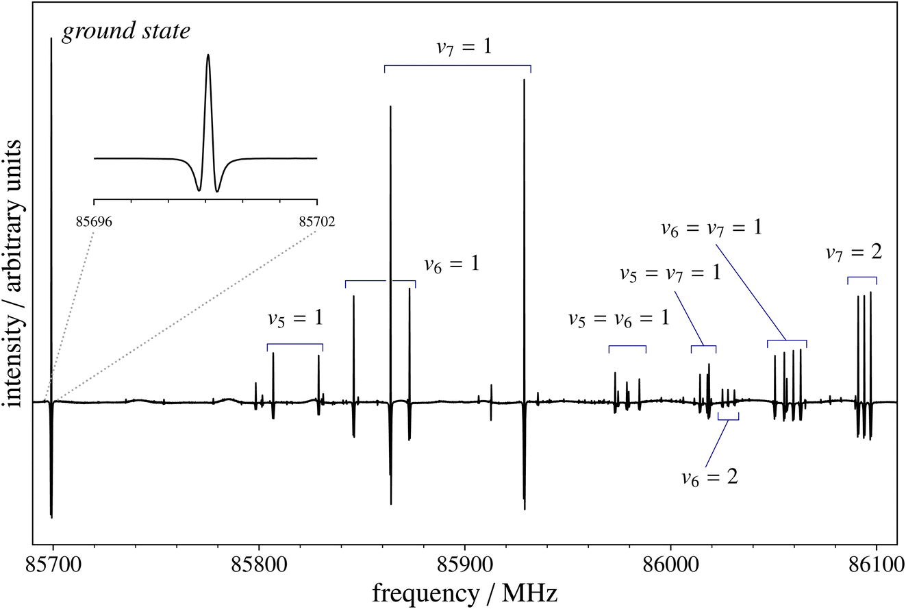 | ||
| Fig. 3 Recording of the J = 31 ← 30 transition of 35ClC3N. The strong leftmost feature belongs to the rotational spectrum in the vibrational ground state (also shown in the inset with a magnified x-axis scale). Several multiplets belonging to the rotational spectra in vibrational excited states due to the fundamentals, overtones, and combinations of the v5, v6, and v7 bending modes are clearly visible towards higher frequencies. | ||
| Constant | Unit | This work | Ref. 74 | |
|---|---|---|---|---|
| Exp.a | Theo.b | |||
| a Numbers in parentheses are one standard deviation in units of the last quoted digit. The “fix” superscript note indicates values held fixed at their computed value. b Rotational constants at the CCSD(T)/CBS+CV level augmented by fc-CCSD(T)/cc-pVTZ vibrational corrections. Quartic and sextic centrifugal distortion constants are at the ae-CCSD(T)/cc-pCVTZ and fc-CCSD(T)/cc-pVTZ levels, respectively. Nuclear quadrupole coupling constants at the ae-CCSD(T)/cc-pCVQZ level. | ||||
| 35ClC3N | ||||
| B 0 | MHz | 1382.32357(35) | 1382.35 | 1382.328(2) |
| D J | kHz | 41.51(14) | 39.6 | 0.054(5) |
| H J | mHz | −0.3fix | −0.3 | — |
| χ(Cl) | MHz | — | −78.74 | −75(4) |
| χ(N) | MHz | — | −4.28 | — |
|
||||
| 37ClC3N | ||||
| B 0 | MHz | 1350.35289(25) | 1350.38 | 1350.360(2) |
| D J | kHz | 39.835(92) | 37.9 | 0.054(5) |
| H J | mHz | −0.3fix | −0.3 | — |
| χ(Cl) | MHz | — | −62.06 | −62(3) |
| χ(N) | MHz | — | −4.28 | — |
The results collected in Table 2 point out the need of measurements at higher frequency in order to improve rotational constant determination, which is also related to the derivation of an improved value of the quartic centrifugal distortion constant. In this respect, it is interesting to note that, while our measurements are not able to determine the sextic centrifugal distortion constant with a meaningful uncertainty, it is necessary to fix it at the computed value in order to improve the fit (and thus reproduce transition frequencies within their experimental error) and obtain the correct ratio for the D values of the two isotopic species. This simple example shows the important role played by accurate quantum-chemical computations also for guiding the fitting procedure for the derivation of the experimental spectroscopic parameters. Focusing on computational results, it is worth noting that, for both isotopologues, the rotational constant is predicted with a deviation as small as 0.002% (which means about 30 kHz in absolute terms). The error increases to 5% for the quartic centrifugal distortion constant, but still the accuracy is good enough to guide experiment and in particular, as mentioned above, to provide the reference value for the D(35ClC3N)/D(37ClC3N) ratio. In Table 2, the nuclear quadrupole coupling constants are also reported. The only experimental values available are for χ(35Cl) and χ(37Cl), and they come from ref. 74. The experimental error is quite large (about 5%) and, according to the literature on this topic,37,51,73,77 the computed values are probably more accurate.
The present work allowed us to set up an accurate line catalog to support astronomical observations, with transition frequencies predicted with the proper accuracy (i.e. uncertainties smaller than 100 kHz) up to 250 GHz. Even if only seven molecules containing chlorine have been detected in space,5 the detection of CH3Cl towards IRAS 16293 (ALMA observations) and in the coma of the 67P/Churyumov–Gerasimenko comet (ROSINA mass spectrometry measurements)78 suggests that polyatomic molecules with chlorine can be discovered in the ISM.
In ref. 75, the rotational spectra of all single-substituted isotopologues of three linear cyanopolyynes, namely HC7N, HC9N, and HC11N, have been investigated in the 6–18 GHz frequency range. These molecules were produced by high-voltage low-current discharge. Of interest to this work, the rotational transitions of DC7N with J values varying from 6 to 12 were recorded, with the hyperfine structure due to N being resolved. The results obtained are collected in Table 3 together with the present experimental and computational outcomes.
| Constant | Unit | This work | Ref. 75 | |
|---|---|---|---|---|
| Exp.a | Theo.b | |||
| a Numbers in parentheses are one standard deviation in units of the last quoted digit. b Rotational constant from the TM+LR approach augmented by fc-MP2/cc-pVDZ vibrational correction. Quartic and sextic centrifugal distortion constants at the fc-MP2/cc-pVDZ level. Nuclear quadrupole coupling constants at the ae-CCSD(T)/cc-pCVTZ level on top of the TM+LR structure. | ||||
| B 0 | MHz | 545.3151998(89) | 545.47 | 545.31523(7) |
| D J | Hz | 3.7241(27) | 2.98 | 3.85(28) |
| H J | nHz | — | 0.86 | — |
| χ(N) | MHz | −4.315(87) | −4.21 | −4.33(22) |
| χ(D) | MHz | — | −0.18 | — |
In our experiment, DC7N has been produced by FVP as explained in the Methods section. Measurements have been performed in the 80–90 GHz range (with transition frequencies retrieved with 15 kHz accuracy) and merged in a global fit together with those (7.6–14.2 GHz) from ref. 75. Incorporation of millimeter-wave measurements in the fit has led to crucial improvement in the accuracy of the spectroscopic parameters (B0 and DJ by one and two orders of magnitude, respectively) as well as in the line catalog. For example, transitions lying at about 100 GHz are predicted with an uncertainty of 0.9–1 MHz by the spectroscopic parameters of ref. 75 (see Cologne database catalog: https://cdms.astro.uni-koeln.de/cgi-bin/cdmssearch?file=c100502.cat), while the present work allows the prediction of the same lines with an uncertainty of about 10 kHz, with the modification in the transition frequencies (with respect to the Cologne database catalog22) of about 500 kHz. Such changes are relevant even for a long carbon chain like DC7N because at temperatures of 100–200 K the most intense rotational transitions lies in the millimeter-wave region. Since our measurements involve high J values (ranging from 75 to 81), the hyperfine structure due to nitrogen could not be resolved. However, the improvement in the determination of the quartic centrifugal distortion constant also reduces the error affecting the nitrogen quadrupole coupling constant (because of a better constraint of the experimental data).
DC7N provides a significant testing ground for the TM+LR approach described in the Methods section. The TM+LR structure, derived as explained in the methodology section, is reported in Fig. 4, where it is compared with the CCSD(T) geometry by Botschwina et al.76 and the effective r0 structure determined in ref. 75. In ref. 76, a fc-CCSD(T)/cc-pVTZ optimized geometry was empirically corrected by reducing the CH bond length by 0.0019 Å, triple CC bonds by 0.0064 Å, single CC bonds by 0.0060 Å, and the CN bond distance by 0.0069 Å. These corrections were meant to account for basis-set truncation and core-correlation effects. Despite the empiric nature of these corrections, the “corrected CCSD(T)/cc-pVTZ” structure shows only small deviations (about 2 to 5 mÅ) from our TM+LR equilibrium geometry. This has, however, a small but non-negligible impact on the rotational constant. As can be seen in Table 3, our theoretical prediction overestimates the experimental B0 by only 158 kHz, which means less than 0.03% in relative terms. Using our computed vibrational correction (at the fc-MP2/cc-pVDZ level), the structure by Botschwina et al. leads to a B0 underestimated by 0.05%. However, it has to be emphasized that our result has been obtained at the price of an extremely limited computational cost. The final comment concerns the experimental effective (r0) structure obtained from a least-square fit of the rotational constants of all single-substituted isotopologues. In this case, larger deviations from our TM+LR structure are noted, thus pointing out that vibrational effects need to be explicitly taken into account by means of the SE approach.37
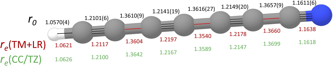 | ||
| Fig. 4 Molecular structure of HC7N. The effective structure (r0) from ref. 75 and the corrected CCSD(T)/cc-pVTZ equilibrium geometry (in green; see text for details) from ref. 76 are compared to the TM+LR equilibrium structure (in red; this work. Bonds are depicted along the carbon chain: in black those corrected using the TM approach, in red those incorporating the LR correction). | ||
3.2 Radical species: CCS and CH2CN
For the first time in our lab, FVP has been employed to produce a radical species. The cyanomethyl radical, CH2CN, has been produced using a 90 cm tubular furnace (see Methods for details) and starting from a small amount (about 3 mTorr, 0.4 Pa) of CH3CN with the oven temperature set at 950 °C, with measurements performed as above in a constant flow of gas. An example of rotational spectrum recording is provided in Fig. 5, where it is noted that a good S/N could be obtained. The rotational spectrum of CH2CN has already been well characterized in the centimeter-79 and millimeter-wave80 region. The first experimental work dates back to 1988 (ref. 81) and immediately led to the detection of CH2CN in the ISM.82 In ref. 80,81, the cyanomethyl radical was prepared using a DC discharge technique, as usually done in frequency-domain spectrometers.26,83–86 In the microwave regime, where time-domain rotational spectroscopy is exploited, CH2CN was produced using a pulsed-discharge nozzle.79 While a flash pyrolysis microreactor exploiting a Chen nozzle combined with a broadband microwave spectrometer is a well established technique for the investigation of the rotational spectrum of radicals (see, for example, ref. 87 and 88), in millimeter-wave direct absorption spectrometers, employment of pyrolysis is very limited and only very few examples can be found in the literature.89 However, our first application is very promising, with production conditions being easier to control and adjust with respect to DC discharge.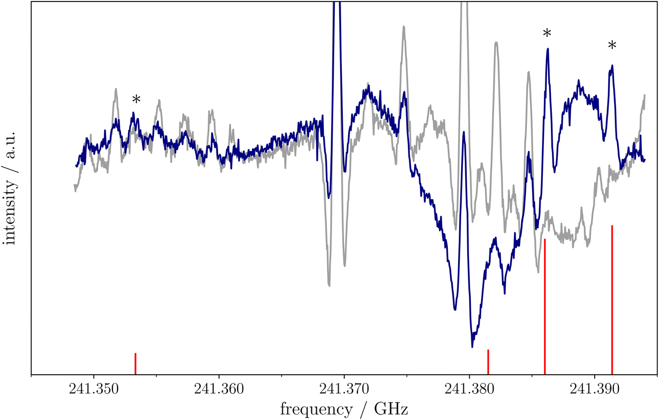 | ||
| Fig. 5 Small portion of the CH3CN spectrum around 241.37 GHz. The dark blue profile has been obtained with the oven temperature set at 950 °C: the lines belonging to the CH2CN radical are made evident by asterisks. The grey profile is the recording with the FVP oven switched off. | ||
First detections of the CCS radical date back to 1987 and refer to the TMC-1 molecular cloud91 and the envelope of the C-rich star IRC+10216.92 Subsequently, the characterization of the rotational spectrum of CCS was extended to the millimeter-wave region up to 292 GHz.90 However, extrapolations to frequencies much higher than 300 GHz should be viewed with caution. For this reason, with the aim of further improving its spectroscopic parameters and thus the line catalog to be used for astronomical observations, we have extended the analysis of the CCS rotational spectrum up to 686 GHz, this radical being produced by DC discharge as explained in the Methods section. The results of our spectroscopic analysis, which collects all data available on CCS, are reported in Table 4, where they are compared with those from ref. 90. The highly accurate computed parameters obtained in ref. 36 are also given. Concerning the latter, while interested readers are referred to the original paper, we recall that the equilibrium rotational constant was obtained at the CCSD(T)/CBS+CV+fT+fQ level (which incorporates into the CCSD(T)/CBS+CV approach, described in the Methods section, the effect of full treatment of triple and quadruple excitations) and corrected for vibrational effects at the ae-CCSD(T)/cc-pCVQZ level, which also provided the quartic and sextic centrifugal distortion constants. The comparison of Table 4 points out that the new measurements allowed us to improve all spectroscopic parameters and determine the sextic centrifugal distortion constant for the first time. It is also worth noting that the state-of-the-art computations of ref. 36 allowed the prediction of B0 with an accuracy of 0.005%.
| Constant/unit | This work | Ref. 36 | Ref. 90 |
|---|---|---|---|
| Exp.a | Theo.b | Exp.a | |
| a Numbers in parentheses are one standard deviation in units of the last quoted digit. b For details, see ref. 36. | |||
| B 0/MHz | 6477.75023(15) | 6477.403 | 6477.75036(71) |
| D J/kHz | 1.72791(18) | 1.6 | 1.72796(95) |
| H J/mHz | 0.330(47) | 0.02 | — |
| λ/MHz | 97195.69(14) |
— | 97196.07(77) |
| λ D/kHz | 26.97(17) | — | 27.00(67) |
| γ/MHz | −14.7159(88) | −12.1 | −14.737(49) |
| γ D/mHz | 43.4(46) | — | 55(37) |
CCS is a 3Σ− radical in its electronic ground state. In such a case, the total angular momentum J is given by the coupling between the molecular angular momentum N and the electronic spin momentum S. The effective Hamiltonian operator thus contains three terms: in addition to the rotational Hamiltonian, with N being the associated quantum number (different from the J symbol used for closed-shell species), there are the Hamiltonians describing the electron spin-rotation and spin–spin interactions. The corresponding spectroscopic parameters are γ and λ, namely the electron spin-rotation and the spin–spin interaction constants, respectively, with γD and λD representing their centrifugal distortion correction. From Table 4, it is noted that γ and λ are determined with high accuracy and that their centrifugal distortion dependence needs to be incorporated in order to reproduce the recorded transitions within their experimental accuracy. Concerning the latter, for our measurements, uncertainty varies from 50 kHz to 100 kHz depending on the intensity and S/N. The largest value applies to the fine component of the highest transition recorded at 685.5 GHz.
4 Conclusions
In this work, an overview of the strategy exploited at the ROT&Comp laboratory of the Department of Chemistry “Giacomo Ciamician”, University of Bologna, for the spectroscopic characterization of unstable and reactive species has been provided. This strategy relies on the strong interplay of experiment and theory in the field of rotational spectroscopy. The examples addressed point out that our computational methodology is able to predict rotational constants with uncertainties well below 0.05% and the other spectroscopic parameters with discrepancies with respect to experiment of the order of a few percents. Consequently, computed spectroscopic parameters and predicted spectra are powerful tools for guiding the recording, the assignment and the analysis of the rotational spectra as well as for providing reliable data for missing information. The experimental analysis in terms of an effective Watson-type Hamiltonian then leads to the set up of spectroscopic line catalogs, where transition frequencies are provided with uncertainties ranging from a few kHz to a maximum of 100–150 kHz. Therefore, these line catalogs are highly suitable for guiding astronomical searches.Author contributions
CP contributed to the conceptualization, project administration, methodology, data curation, validation, writing – original draft, writing – review & editing, and funding acquisition. SA, LB and MM contributed to the investigation, data curation, formal analysis, validation, and writing – review & editing.Conflicts of interest
There are no conflicts to declare.Acknowledgements
This work has been supported by MUR (PRIN Grant Number 202082CE3T) and by the University of Bologna (RFO funds). The COST Action CA21101 “COSY – Confined molecular systems: from a new generation of materials to the stars” is also acknowledged.Notes and references
- S. Yamamoto, Introduction to Astrochemistry: Chemical Evolution from Interstellar Clouds to Star and Planet Formation, 2017 Search PubMed.
- A. Negron-Mendoza and S. Ramos-Bernal, First Steps in the Origin of Life in the Universe, Dordrecht, 2001, pp. 145–150 Search PubMed.
- C. Puzzarini, Front. Astron. Space Sci., 2020, 7, 19 CrossRef.
- E. Herbst, Front. Astron. Space Sci., 2021, 8, 776942 CrossRef.
- B. A. McGuire, Astrophys. J., Suppl. Ser., 2022, 259, 30 CrossRef.
- B. A. McGuire, A. M. Burkhardt, C. N. Shingledecker, S. V. Kalenskii, E. Herbst, A. J. Remijan and M. C. McCarthy, Astrophys. J., Lett., 2017, 843, L28 CrossRef.
- J. Cernicharo, M. Agúndez, C. Cabezas, B. Tercero, N. Marcelino, R. Fuentetaja, J. R. Pardo and P. de Vicente, Astron. Astrophys., 2021, 656, L21 CrossRef CAS.
- S. Brünken, H. Gupta, C. A. Gottlieb, M. C. McCarthy and P. Thaddeus, Astrophys. J., 2007, 664, L43 CrossRef.
- A. J. Remijan, J. M. Hollis, F. J. Lovas, M. A. Cordiner, T. J. Millar, A. J. Markwick-Kemper and P. R. Jewell, Astrophys. J., 2007, 664, L47 CrossRef CAS.
- N. W. Broten, T. Oka, L. W. Avery, J. M. MacLeod and H. W. Kroto, Astrophys. J., Lett., 1978, 223, L105–L107 CrossRef CAS.
- N. Marcelino, M. Agúndez, B. Tercero, C. Cabezas, C. Bermúdez, J. D. Gallego, P. deVicente and J. Cernicharo, Astron. Astrophys., 2020, 643, L6 CrossRef PubMed.
- D. Alberton, L. Bizzocchi, N. Jiang, M. Melosso, V. M. Rivilla, A. P. Charmet, B. M. Giuliano, P. Caselli, C. Puzzarini, S. Alessandrini, L. Dore, I. Jiménez-Serra and J. Martín-Pintado, Astron. Astrophys., 2023, 669, A93 CrossRef CAS.
- V. M. Rivilla, L. Colzi, I. Jiménez-Serra, J. Martín-Pintado, A. Megías, M. Melosso, L. Bizzocchi, Á. López-Gallifa, A. Martínez-Henares, S. Massalkhi, B. Tercero, P. de Vicente, J.-C. Guillemin, J. G. de la Concepción, F. Rico-Villas, S. Zeng, S. Martín, M. A. Requena-Torres, F. Tonolo, S. Alessandrini, L. Dore, V. Barone and C. Puzzarini, Astrophys. J., Lett., 2022, 929, L11 CrossRef.
- E. Herbst and E. F. van Dishoeck, Annu. Rev. Astron. Astrophys., 2009, 47, 427–480 CrossRef CAS.
- A. Belloche, A. A. Meshcheryakov, R. T. Garrod, V. V. Ilyushin, E. A. Alekseev, R. A. Motiyenko, L. Margulès, H. S. P. Müller and K. M. Menten, Astron. Astrophys., 2017, 601, A49 CrossRef.
- A. Belloche, R. T. Garrod, H. S. P. Müller, K. M. Menten, I. Medvedev, J. Thomas and Z. Kisiel, Astron. Astrophys., 2019, 628, A10 CrossRef CAS.
- I. Jiménez-Serra, J. Martín-Pintado, V. M. Rivilla, L. Rodríguez-Almeida, E. R. Alonso Alonso, S. Zeng, E. J. Cocinero, S. Martín, M. Requena-Torres, R. Martín-Domenech and L. Testi, Astrobiology, 2020, 20, 1048–1066 CrossRef PubMed.
- V. M. Rivilla, I. Jiménez-Serra, J. Martín-Pintado, C. Briones, L. F. Rodríguez-Almeida, F. Rico-Villas, B. Tercero, S. Zeng, L. Colzi, P. de Vicente, S. Martín and M. A. Requena-Torres, Proc. Natl. Acad. Sci. U. S. A., 2021, 118, e2101314118 CrossRef CAS PubMed.
- A. Belloche, R. T. Garrod, O. Zingsheim, H. S. P. Müller and K. M. Menten, Astron. Astrophys., 2022, 662, A110 CrossRef CAS.
- I. Jiménez-Serra, L. F. Rodríguez-Almeida, J. Martín-Pintado, V. M. Rivilla, M. Melosso, S. Zeng, L. Colzi, Y. Kawashima, E. Hirota, C. Puzzarini, B. Tercero, P. de Vicente, F. Rico-Villas, M. A. Requena-Torres and S. Martín, Astron. Astrophys., 2022, 663, A181 CrossRef.
- B. A. McGuire, Astrophys. J., Suppl. Ser., 2018, 239, 17 CrossRef CAS.
- H. S. P. Müller, F. Schlöder, J. Stutzki and G. Winnewisser, J. Mol. Struct., 2005, 742, 215–227 CrossRef.
- J. Tennyson, Astronomical Spectroscopy. An Introduction to the Atomic and Molecular Physics of Astronomical Spectroscopy, 2019 Search PubMed.
- R. C. Woods, J. Mol. Struct., 1983, 97, 195–202 CrossRef CAS.
- G. Cazzoli, L. Cludi, G. Buffa and C. Puzzarini, Astrophys. J., Suppl. Ser., 2012, 203, 11 CrossRef.
- G. Cazzoli, V. Lattanzi, T. Kirsch, J. Gauss, B. Tercero, J. Cernicharo and C. Puzzarini, Astron. Astrophys., 2016, 591, A126 CrossRef PubMed.
- G. Winnewisser, F. Lewen, S. Thorwirth, M. Behnke, J. Hahn, J. Gauss and E. Herbst, Chem.–Eur. J., 2003, 9, 5501–5510 CrossRef CAS PubMed.
- M. Melosso, L. Bizzocchi, H. Gazzeh, F. Tonolo, J.-C. Guillemin, S. Alessandrini, V. M. Rivilla, L. Dore, V. Barone and C. Puzzarini, Chem. Commun., 2022, 58, 2750–2753 RSC.
- A. Melli, M. Melosso, L. Bizzocchi, S. Alessandrini, N. Jiang, F. Tonolo, S. Boi, G. Castellan, C. Sapienza, J.-C. Guillemin, L. Dore and C. Puzzarini, J. Phys. Chem. A, 2022, 126, 6210–6220 CrossRef CAS PubMed.
- M. Melosso, B. Conversazioni, C. Degli Esposti, L. Dore, E. Cané, F. Tamassia and L. Bizzocchi, J. Quant. Spectrosc. Radiat. Transfer, 2019, 222, 186–189 CrossRef.
- M. Melosso, L. Bizzocchi, F. Tamassia, C. Degli Esposti, E. Canè and L. Dore, Phys. Chem. Chem. Phys., 2019, 21, 3564–3573 RSC.
- N. Jiang, M. Melosso, F. Tamassia, L. Bizzocchi, L. Dore, E. Canè, D. Fedele, J.-C. Guillemin and C. Puzzarini, Front. Astron. Space Sci., 2021, 8, 29 Search PubMed.
- W. Gordy and R. L. Cook, Microwave Molecular Spectra, Wiley, New York, 1984 Search PubMed.
- C. Puzzarini, M. Heckert and J. Gauss, J. Chem. Phys., 2008, 128, 194108 CrossRef PubMed.
- C. Puzzarini and J. F. Stanton, Phys. Chem. Chem. Phys., 2023, 25, 1421–1429 RSC.
- S. Alessandrini, J. Gauss and C. Puzzarini, J. Chem. Theory Comput., 2018, 14, 5360–5371 CrossRef CAS PubMed.
- C. Puzzarini, J. F. Stanton and J. Gauss, Int. Rev. Phys. Chem., 2010, 29, 273–367 Search PubMed.
- T. Helgaker, P. Jørgensen and J. Olsen, Electronic-Structure Theory, Wiley, Chichester, 2000 Search PubMed.
- M. Heckert, M. Kállay and J. Gauss, Mol. Phys., 2005, 103, 2109 CrossRef CAS.
- M. Heckert, M. Kállay, D. P. Tew, W. Klopper and J. Gauss, J. Chem. Phys., 2006, 125, 044108 CrossRef PubMed.
- C. Puzzarini and V. Barone, Phys. Chem. Chem. Phys., 2011, 13, 7189–7197 RSC.
- A. G. Császár, W. D. Allen and H. F. Schaefer III, J. Chem. Phys., 1998, 108, 9751–9764 CrossRef.
- A. Karton, E. Rabinovich, J. M. L. Martin and B. Ruscic, J. Chem. Phys., 2006, 125, 144108 CrossRef PubMed.
- A. Karton and J. M. L. Martin, J. Chem. Phys., 2012, 136, 124114 CrossRef PubMed.
- A. Tajti, P. G. Szalay, A. G. Császár, M. Kállay, J. Gauss, E. F. Valeev, B. A. Flowers, J. Vázquez and J. F. Stanton, J. Chem. Phys., 2004, 121, 11599–11613 CrossRef CAS PubMed.
- K. A. Peterson, D. Feller and D. Dixon, Theor. Chem. Acc., 2012, 113, 1079 Search PubMed.
- W. J. Morgan, D. A. Matthews, M. Ringholm, J. Agarwal, J. Z. Gong, K. Ruud, W. D. Allen, J. F. Stanton and H. F. Schaefer, J. Chem. Theory Comput., 2018, 14, 1333–1350 CrossRef CAS PubMed.
- J. Lupi, S. Alessandrini, V. Barone and C. Puzzarini, J. Chem. Theory Comput., 2021, 17, 6974–6992 CrossRef CAS PubMed.
- X. Huang and T. J. Lee, J. Chem. Phys., 2009, 131, 104301 CrossRef.
- Q. Cheng, R. C. Fortenberry and N. J. DeYonker, J. Chem. Phys., 2017, 147, 234303 CrossRef PubMed.
- C. Puzzarini, J. Bloino, N. Tasinato and V. Barone, Chem. Rev., 2019, 119, 8131–8191 CrossRef CAS PubMed.
- D. A. Matthews, L. Cheng, M. E. Harding, F. Lipparini, S. Stopkowicz, T.-C. Jagau, P. G. Szalay, J. Gauss and J. F. Stanton, J. Chem. Phys., 2020, 152, 214108 CrossRef CAS PubMed.
- K. Raghavachari, G. W. Trucks, J. A. Pople and M. Head-Gordon, Chem. Phys. Lett., 1989, 157, 479–483 CrossRef CAS.
- D. Feller, J. Chem. Phys., 1993, 98, 7059–7071 CrossRef CAS.
- T. Helgaker, W. Klopper, H. Koch and J. Noga, J. Chem. Phys., 1997, 106, 9639–9646 CrossRef CAS.
- T. H. Dunning Jr, J. Chem. Phys., 1989, 90, 1007–1023 CrossRef.
- A. K. Wilson, T. van Mourik and T. H. Dunning Jr, J. Mol. Struct.: THEOCHEM, 1996, 388, 339–349 CrossRef CAS.
- D. E. Woon and T. H. Dunning Jr, J. Chem. Phys., 1995, 103, 4572–4585 CrossRef CAS.
- K. A. Peterson and T. H. Dunning Jr, J. Chem. Phys., 2002, 117, 10548–10560 CrossRef CAS.
- C. Møller and M. S. Plesset, Phys. Rev., 1934, 46, 618 CrossRef.
- H. Ye, S. Alessandrini, M. Melosso and C. Puzzarini, Phys. Chem. Chem. Phys., 2022, 24, 23254–23264 RSC.
- A. Melli, F. Tonolo, V. Barone and C. Puzzarini, J. Phys. Chem. A, 2021, 125, 9904–9916 CrossRef CAS PubMed.
- M. Piccardo, E. Penocchio, C. Puzzarini, M. Biczysko and V. Barone, J. Phys. Chem. A, 2015, 119, 2058–2082 CrossRef CAS PubMed.
- E. Penocchio, M. Piccardo and V. Barone, J. Chem. Theory Comput., 2015, 11, 4689–4707 CrossRef CAS PubMed.
- G. Ceselin, V. Barone and N. Tasinato, J. Chem. Theory Comput., 2021, 17, 7290–7311 CrossRef CAS PubMed.
- P. Pulay, W. Meyer and J. E. Boggs, J. Chem. Phys., 1978, 68, 5077–5085 CrossRef CAS.
- J. Demaison, J. E. Boggs and A. G. Császár, Equilibrium Molecular Structures: from Spectroscopy to Quantum Chemistry, CRC Press, 2016 Search PubMed.
- G. Santra, N. Sylvetsky and J. M. L. Martin, J. Phys. Chem. A, 2019, 123, 5129–5143 CrossRef CAS PubMed.
- E. Papajak, J. Zheng, X. Xu, H. R. Leverentz and D. G. Truhlar, J. Chem. Theory Comput., 2011, 7, 3027–3034 CrossRef CAS PubMed.
- S. Grimme, J. Antony, S. Ehrlich and H. Krieg, J. Chem. Phys., 2010, 132, 154104 CrossRef PubMed.
- S. Grimme, S. Ehrlich and L. Goerigk, J. Comput. Chem., 2011, 32, 1456–1465 CrossRef CAS PubMed.
- I. M. Mills, in Molecular Spectroscopy: Modern Research, ed. K. N. Rao and C. W. Matthews, Academic Press, 1972, vol. 1, pp. 115–140 Search PubMed.
- C. Puzzarini, G. Cazzoli, M. E. Harding, J. Vázquez and J. Gauss, J. Chem. Phys., 2009, 131, 234304 CrossRef PubMed.
- T. Bjorvatten, J. Mol. Struct., 1974, 20, 75–82 CrossRef CAS.
- M. C. McCarthy, E. S. Levine, A. J. Apponi and P. Thaddeus, J. Mol. Spectrosc., 2000, 203, 75–81 CrossRef CAS PubMed.
- P. Botschwina, M. Horn, K. Markey and R. Oswald, Mol. Phys., 1997, 92, 381–392 CrossRef CAS.
- G. Cazzoli, C. Puzzarini and J. Gauss, Mol. Phys., 2012, 110, 2359–2369 CrossRef CAS.
- E. C. Fayolle, K. I. Öberg, J. K. Jørgensen, K. Altwegg, H. Calcutt, H. S. P. Müller, M. Rubin, M. H. D. van der Wiel, P. Bjerkeli, T. L. Bourke, A. Coutens, E. F. van Dishoeck, M. N. Drozdovskaya, R. T. Garrod, N. F. W. Ligterink, M. V. Persson, S. F. Wampfler and R. Team, Nat. Astron., 2017, 1, 703–708 CrossRef.
- H. Ozeki, T. Hirao, S. Saito and S. Yamamoto, Astrophys. J., 2004, 617, 680 CrossRef CAS.
- S. Saito and S. Yamamoto, J. Chem. Phys., 1997, 107, 1732–1739 CrossRef CAS.
- S. Saito, S. Yamamoto, W. M. Irvine, L. M. Ziurys, H. Suzuki, M. Ohishi and N. Kaifu, Astrophys. J.,Lett., 1988, 334, L113–L116 CrossRef CAS PubMed.
- W. M. Irvine, P. Friberg, A. Hjalmarson, S. Ishikawa, N. Kaifu, K. Kawaguchi, S. C. Madden, H. E. Matthews, M. Ohishi, S. Saito, H. Suzuki, P. Thaddeus, B. E. Turner, S. Yamamoto and L. M. Ziurys, Astrophys. J., Lett., 1988, 334, L107–L111 CrossRef CAS PubMed.
- Y. Endo, S. Saito and E. Hirota, J. Mol. Spectrosc., 1982, 92, 443–450 CrossRef CAS.
- R. J. McMahon, M. C. McCarthy, C. A. Gottlieb, J. B. Dudek, J. F. Stanton and P. Thaddeus, Astrophys. J., 2003, 590, L61 CrossRef CAS.
- H. Ozeki, S. Bailleux and G. Wlodarczak, Astron. Astrophys., 2011, 527, A64 CrossRef.
- L. Bizzocchi, M. Melosso, B. M. Giuliano, L. Dore, F. Tamassia, M.-A. Martin-Drumel, O. Pirali, L. Margulès and P. Caselli, Astrophys. J., Suppl. Ser., 2020, 247, 59 CrossRef CAS.
- N. M. Kidwell, V. Vaquero-Vara, T. K. Ormond, G. T. Buckingham, D. Zhang, D. N. Mehta-Hurt, L. McCaslin, M. R. Nimlos, J. W. Daily, B. C. Dian, J. F. Stanton, G. B. Ellison and T. S. Zwier, J. Phys. Chem. Lett., 2014, 5, 2201–2207 CrossRef CAS PubMed.
- C. Abeysekera, A. Hernandez-Castillo, J. F. Stanton and T. S. Zwier, J. Phys. Chem. A, 2018, 122, 6879–6885 CrossRef CAS PubMed.
- L. Kolesniková, J. Varga, L. N. Stříteská, H. Beckers, H. Willner, F. Aubke and s. Urban, J. Chem. Phys., 2009, 130, 184309 CrossRef PubMed.
- S. Yamamoto, S. Saito, K. Kawaguchi, Y. Chikada, H. Suzuki, N. Kaifu, S.-I. Ishikawa and M. Ohishi, Astrophys. J., 1990, 361, 318 CrossRef CAS.
- S. Saito, K. Kawaguchi, S. Yamamoto, M. Ohishi, H. Suzuki and N. Kaifu, Astrophys. J., Lett., 1987, 317, L115 CrossRef CAS.
- J. Cernicharo, M. Guelin, H. Hein and C. Kahane, Astron. Astrophys., 1987, 181, L9–L12 CAS.
Footnote |
| † Electronic supplementary information (ESI) available. See DOI: https://doi.org/10.1039/d3fd00052d |
| This journal is © The Royal Society of Chemistry 2023 |