
Monitoring the risk of Legionella infection using a general Bayesian network updated from temporal measurements in agricultural irrigation with reclaimed wastewater†
Gaspar
Massiot
 *ab,
Dominique
Courault
c,
Pauline
Jacob
d and
Isabelle
Albert
b
*ab,
Dominique
Courault
c,
Pauline
Jacob
d and
Isabelle
Albert
b
aUMR AgroParisTech/INRAE Silva, INRAE-AgroParisTech-Université de Lorraine, 54000, Nancy, France. E-mail: gaspar.massiot@agroparistech.fr
bUniversité Paris-Saclay, AgroParisTech, INRAE, UMR MIA Paris-Saclay, 91120, Palaiseau, France
cUMR 1114 EMMAH, INRAE, Site Agroparc, CS 40509, 84914 Avignon, France
dVeolia Recherche & Innovation, Chemin de la Digue, 78600 Maisons-Laffitte, France
First published on 24th November 2022
Abstract
Reuse of reclaimed wastewater for agricultural irrigation is an expanding practice worldwide. This practice needs to be monitored, partly because of pathogens that the water may contain after treatments. More particularly, sprinkler irrigation is known to generate aerosols which may lead to severe health risks to the population close to irrigated areas in case of the presence of Legionella bacteria in the water. A pilot experiment was conducted on two corn fields in South-Western France, irrigated with wastewater undergoing two different water treatments (ultra-filtration and UV). Water analyses have shown high levels of Legionella in the water even after a standard wastewater treatment plant (WWTP) cleaning process followed by the UV treatment (up to 106 GC per L in 2019). In this context, an updated general Bayesian network (GBN), using discrete and continuous random variables, in quantitative microbial risk assessment (QMRA) is proposed to monitor the risk of Legionella infection in the vicinity of the irrigated plots. The model's originality is based on i) a graphical probabilistic model that describes the exposure pathway of Legionella from the WWTP to the population using observed and non-observed variables and ii) the model inference updating at each new available measurement. Different scenarios are simulated according to the exposure time of the persons, taking into account various distances from the emission source and a large dataset of climatic data. From the learning process included in the Bayesian principle, quantities of interest (contaminations before and after water treatments, inhaled dose, probabilities of infection) can be quantified with their uncertainty before and after the inclusion of each new data collected in situ. This approach gives a rigorous tool that allows monitoring the risks, facilitates discussions with reuse experts and progressively reduces uncertainty quantification through field data accumulation. For the two pilot treatments analyzed in this study, the median annual risk of Legionella infection did not exceed the US EPA annual infection benchmark of 10−4 for any of the population at risk during the past few months of the pilot experiment (DALYs are estimated up to 10−5). The risk still bears watching with support from the method shown in this work.
Water impactThis paper presents a model for the risk assessment of pathogen inhalation from sprinkler irrigation using treated wastewater. The approach is applied to Legionella analyzed on a pilot site where two different treatments were performed on water with numerous analyses for monitoring pathogens. |
1 Introduction
In the context of climate change, the growing global water scarcity and more severe and frequent drought events have intensified the need to find alternative water resources.1,2 Reclaimed wastewater is a renewable resource from which renewable energy can be produced, but also materials and water can be recovered.3,4 It is a possible alternative supply to address such water shortages.5 The combination of climate change, population growth and urbanisation has led the European Parliament to foster increased water reuse to alleviate the stress on freshwater supply and prevent the fall in groundwater levels, due in particular to agricultural irrigation,6 which represented more than half of the water used annually in Europe in 2017 according to the European Environment Agency.7However, wastewater reuse still remains uncommon in some countries. Several factors can explain this observation, among them being the pathogens that water may contain, which resulted in strict reuse guidelines. Adegoke et al. (2018)8 have reported the different pathogens found in wastewaters and the associated risks. Quality indicators are commonly used, but they are more and more debated on their representativeness (particularly for viruses and Legionella, e.g., they are not explicitly taken into account as indicators despite their wide occurrence in the environment). Pragmatic recommendations and guidelines were defined by the World Health Organization (WHO)9–12 on the basis of health risk considerations. The new European regulations on minimum requirements for water reuse for agricultural irrigation will take effect on 26 June 2023.13
Sprinkler irrigation with reclaimed wastewater is widely practiced throughout the world but may enhance hazards relative to the dispersion of pathogens by bioaerosols.14–16 A collective expertise appraisal has been performed by ANSES in 2012,17 which assessed various secondary risks (e.g. ingestion) and pointed out the lack of knowledge on health risks, particularly due to pathogen inhalation.
An experiment has been conducted in South-Western France to evaluate the impact of two different treatments on the quality of water reused for sprinkler irrigation of two corn fields (SmartFertiReuse project, https://www.smartfertireuse.fr/, accessed on October 4th 2022), controlling the population risks. Among the different analyzed pathogens in the water, Legionella was found at a high level both at the entrance and output of the wastewater treatment plant (WWTP) (up to 107 GC per L). In the new EU regulations, criteria have been defined for water quality. The minimum required value for Legionella has been set to <1000 CFU L−1 for a reclaimed water class A used for food culture irrigation. These rules are expected to stimulate and facilitate water reuse in the EU and shall also be accompanied by appropriate monitoring of the health risks linked to this practice.
Legionella is an opportunistic bacterium which may be inhaled by humans through water aerosols.18–20Legionella has around 50 species, such as Legionella pneumophila, which is responsible for the most severe infections such as Legionnaire's disease and pneumonia illness (Pontiac fevers).21 These infections due to Legionella pneumophila are particularly problematic for people who have a certain fragility or those who are exposed for a long period to these pathogens and may cause in some cases mortality. In France, an increasing trend of Legionellosis has been observed since 1995.‡ A lot of cases were linked to cooling towers22 but some studies have shown contaminated aerosols by Legionella pneumophila in the vicinity of WWTPs23 and associated diseases have been observed for example in the Netherlands.24
Different approaches have been proposed to quantify health risks applied to Legionella (reviewed by Hamilton et al. (2018)19 and Hamilton et al. (2016)20). Often, there are few observations and numerous authors have shown a wide variability in both space and time of punctual measurements.18,25 It is therefore important to take into account this variability and the uncertainty in risk assessment.
Quantitative microbial risk assessment (QMRA) is an established framework recommended by multiple international organizations (WHO, US EPA, EFSA) to monitor such risks of infection.26 QMRA models have been widely used for food safety management,27 and in the risk assessment of waterborne diseases28–30 due to aerosolisation14,31–34 of water reuse systems,35 and are often coupled with Monte Carlo (MC) simulation approaches which consist of drawing values for all the inputs in the model from distributions defined by external knowledge (e.g., experimental or historical data, expert knowledge) and then propagating these values to all the intermediate variables and outputs through the system in a way that takes the variability and uncertainty of the inputs into account. It is, by definition, a unidirectional approach that prevents the inversion of the dependency relationship between the variables. The Bayesian network (BN) approach, as an alternative to the MC simulation approach in QMRA, overcomes this unidirectional path among other things.36,37 While QMRA may not be able to incorporate the many factors that influence the quantification of the risks (for example, epidemiological data), models based on BNs are an effective framework that addresses this limitation. BN approaches in QMRA provide a powerful approach where the dependency relationship between variables can be inverted (‘backward calculation’, by which the states of the model's variables are updated using ‘downstream’ data).
A BN is a flexible graphical model based on a directed acyclic graph (DAG) where conditional dependencies between the variables are qualitatively represented by directed arcs on the graph38,39 and quantitatively defined with local transition probabilities or deterministic equations. BNs offer transparency and the ability to support causal reasoning based on causal connections. The visual representation in a BN of large quantities of complex information provides an information platform for improved communications with experts through their graphical representation.36,37,40,41 A BN as a system approach encompasses both holistic and modular views, enables the synthesis of knowledge of parts to help understand the whole and makes a complex system more manageable.42 BNs can be applied to a wide range of application domains such as environmental modelling43 and artificial intelligence,44 and as mentioned above to quantitative microbial risk assessment (for a review, see Beaudequin et al. (2015)45), and water reuse and QMRA.41,42,46–48 While QMRAs are often constrained by the availability of required data (for example, in dose–response assessments), system models based on BNs are an effective framework that tackle the lack of data. As all data in the network contribute to the whole, accurate predictions can be made with incomplete data or a quite small sample size.48 BNs were also used for scenario assessment,46 risk minimisation36 and work with uncertainty and variability as a probabilistic tool.41,49
One of the objectives of this paper is the combination of a general Bayesian network (GBN) and QMRA. GBNs, known also as graphical independence networks in the context of continuous and discrete random variables, are a more general case of the BN in which each variable in the data is modelled with a random variable that best suits it, rather than limiting ourselves to multinomial and normal distributions as in other more classical BNs.39,50,51 GBNs can be used as an attractive way of modelling complex systems because they most closely model expert knowledge and data. Due to their ability to incorporate diverse data types, a GBN enables a complex, multivariate statistical problem (such as QMRA) to be efficiently addressed where classical statistical methods are inept. The method allows the integration of a broad range of quantitative or semi-quantitative information, which is particularly useful in domains where traditional experimental and observational data are missing, inaccurate, sparse, or costly. In this paper, compared to other applications in the water reuse and QMRA context previously cited, there is no discretization of the continuous variables in the BN for the learning algorithm. The joint posterior distribution of all the random variables in the BN is obtained by a MCMC (Markov Chain Monte Carlo) algorithm52 as used in computational Bayesian model inference. The powerful capacity of conceptualization available by the BN approach via the graphical network is used to construct the core model36 and the knowledge is updated via computational Bayesian inference via data in the spirit of the Bayesian model approach (see Verbyla et al. (2016)53 in the water reuse QMRA context).
Another objective was the development and application of an updated GBN to monitor health risks associated with exposure to Legionella pneumophila during irrigation events with reclaimed wastewater. The impacts of two types of water treatments were analyzed (described in the following section). Keeping the steady monitoring aspect in mind, the constructed GBN is reevaluated with each arrival of new data. At each step, posterior distributions for all the variables in the model were computed using priors defined as the posterior distributions at the previous step. The final purposes were to assess different risk scenarios according to the population activities, accounting for their distance from the irrigated areas and the environmental conditions in order to get infection probabilities for each configuration.
In the following text, the Materials and methods section describes the study site, the data and the models implemented for the developed risk assessment monitoring tool. The update process of the risk quantification and three scenarios on simulated data are described in the Results section. The update can occur whenever desired and discussed with the experts. The Discussion section discusses the benefits of the developed approach for the continuous monitoring of health risks in the context of QMRA, emphasizing the necessity of informed use of such tools when few data are available.
2 Materials and methods
2.1 Study site and data
A pilot experiment was conducted on an area near Tarbes (43°15′45.78′′N, 0° 5′16.95′′E) where irrigated corn fields from two farms having different agricultural managements have been monitored for various quality criteria since 2018 in the framework of the SmartFertireuse project (FUI SmartFertiReuse project§). Irrigation generally occurs from end of June up to the end of August, with 3, 4 or 5 water supplies of 30–40 mm ha−1. Two different water treatment pilots (ultra-filtration (A) and UV (B)) were installed at the wastewater treatment plant outlet in order to reach the required log reduction after standard treatment of the initial WWTP (stopping only at the secondary level). The different water compartments were sampled at each irrigation date in order to monitor the classical indicators for water quality13 and to quantify Legionella and additional pathogens such as enteric viruses. For each sample, the following were collected: 100 ml at the entrance of the WWTP (6 samples with 2 replicates each), 250 ml after standard WWTP treatments (6 samples with 2 replicates each), 250 ml after A treatment (4 samples with 2 replicates each), 250 ml after B treatment (6 samples with 2 replicates each), and 400 ml at the groundwater (4 samples at each of 2 different sites on the field and with 2 replicates each) for PCR analysis. Additionally, 2 biosamplers (AGI4-Ace Glass incorporated USA, connected to a 12 L min−1 pump), containing 40 ml of ultrapure Milli-Q water, were used to sample bioaerosols in the air above corn during irrigation (see Fig. 1).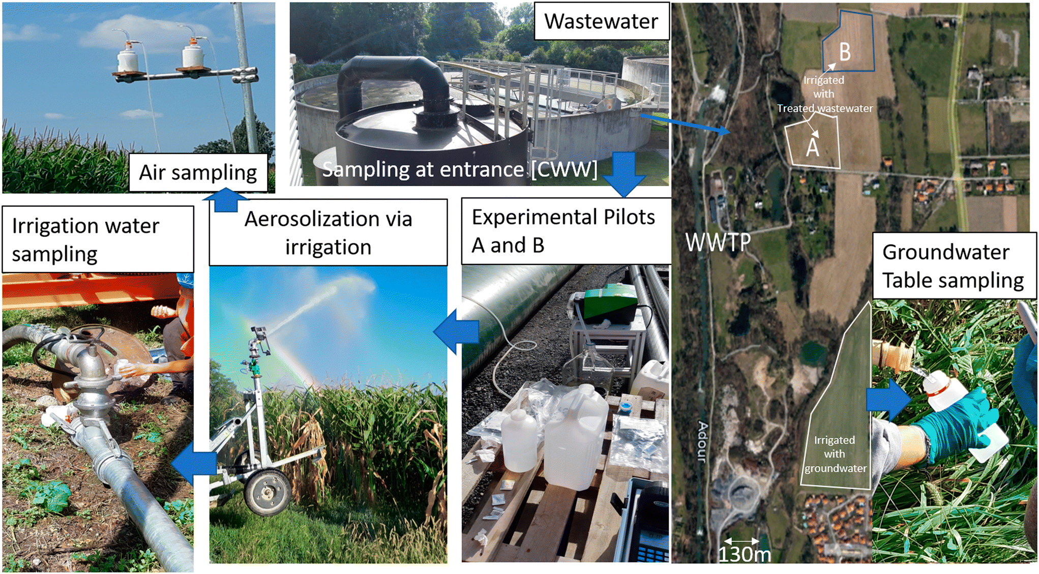 | ||
| Fig. 1 Location of the study site with the monitored fields and the different water sampling. Two fields were irrigated with treated wastewater (the blue arrows show the water transfer from the WWTP, and then the pilot A or B, to the irrigated plots). | ||
All samples were analyzed to quantify Legionella via molecular biology (qPCR from the standard NFT90-471¶). All Legionella species are considered potentially pathogenic for humans, but Legionella pneumophila is the etiological agent responsible for most reported cases of community-acquired and nosocomial legionellosis.54,55 Additionally, some cultivations were made for samples showing high values. Fig. 2 shows the data collected for Legionella spp. presence using the qPCR method and differentiated by sampling zone. The graph presents a large variability between the different analyzed compartments and for the three studied years. As expected, the raw water at the entrance of the WWTP presented the highest values of Legionella and the groundwater had the lowest values from 2019 to 2021. The impact of the two tertiary treatments (A and B) tends to decrease the quantities compared to the values found in raw water. A large variability was also observed according to the dates in 2021 which is difficult to explain. Many factors, including climatic and water storage conditions, can lead to variability. These points will be discussed in the Results section.
 | ||
| Fig. 2 Data collected on site differentiated by sampling zone. Points represent the mean concentration of Legionella spp. for replicates and vertical bars represent their variability. A Complete data from November 2018 to June 2021. B Zoomed in view for the year 2021. | ||
In parallel to these analyses, the meteorological conditions are monitored thanks to a climatic station set up in the area, which records continuously the wind speed and direction, global radiation, air temperature and moisture. To complete this dataset, daily data acquired from the Meteo-France weather station (Tarbes (43°11′12′′N, 0°00′00′′E)) between May and September over the period from 04/29/2010 to 06/18/2020 have been used in order to better take into account the temporal variability of environmental conditions. The crop height was also measured during the irrigation events to assess the aerodynamic roughness (z0) occurring in the atmospheric transport. The values of the crop height varied from 80 cm to 3.2 m for the studied period.
2.2 The QMRA model
The first step of the modelling is to construct a QMRA model that describes the transmission of Legionella along the water exposure pathway described in Fig. 3. | ||
| Fig. 3 Overview of the exposure pathway of Legionella pneumophila in the context of agricultural irrigation of the experimental plots in Tarbes. | ||
1. Irrigation directly from the groundwater table with quality CGT [genome copies per liter (GC per L)], currently in use;
2. Irrigation from wastewater sequentially treated by standard WWTP treatments and experimental pilot A with quality CA [GC per L];
2b. Irrigation from wastewater sequentially treated by standard WWTP treatments and experimental pilot B with quality CB [GC per L].
In the process currently used (part 1 above), the groundwater is not treated in the WWTP before being used for irrigation. In the experimental processes (parts 2 and 2b above), reclaimed wastewater is used. The initial wastewater coming to the WWTP is sequentially treated by standard WWTP treatments and the experimental pilot (A or B). The treatment effects on the water quality are modelled by the following logarithmic decay formulas:
| CA = CTP/10kA, | (1) |
| CB = CTP/10kB, | (2) |
| with CTP = CWW/10kTP, | (3) |
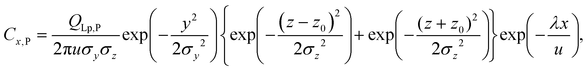
The concentration of Legionella pneumophila CLp,P [GC per L] in each treatment train P ∈ {GT, A, B} was deduced from the concentrations CP above by the following formula:19
| CLp,P = CPfLp, | (4) |
| QLp,P = FSPp150CLp,P3600/103, | (5) |
 | (6) |
• passersby with a supposed average tpasserby of 1 minute of exposure per irrigation day,17
• residents with a supposed average tresident of 2 seconds of exposure over 2.27 hours spent outside per irrigation day,17,57 and
• farmers with a supposed average tfarmer of 30 minutes of exposure per irrigation day (chosen according to the local farmer behavior knowledge).
For each population, the fraction of day the population was exposed was computed and an uncertainty of half a minute around it was considered. For example, tpasserby was taken as a Gaussian distribution centered around 1/(60 × 24) = 6.94 × 10⁻⁴ with a standard deviation of  truncated on [0; 1].
The inhaled dose DA,x,P [genome copies per day] was calculated for each treatment train P, distance x and activity A taking values in {passerby; resident; farmer} as follows:
| DA,x,P = Cx,PItA, | (7) |
| Pi,A,x,P = 1 − e−riDA,x,PfCFU, | (8) |
| Pyear,i,A,x,P = 1 − (1 − Pi,A,x,P)nede, | (9) |
Fig. 4 presents the directed acyclic graph (DAG) of the QMRA model constructed with the equations above. The input distributions (or prior distributions in the Bayesian framework) for each parameter are defined in Table 1.
 | ||
| Fig. 4 Directed acyclic graph of the Bayesian network model. | ||
![[scr N, script letter N]](https://www.rsc.org/images/entities/char_e52d.gif) (μ, σ) denotes the normal distribution of mean μ and standard deviation σ, eventually truncated on the interval T(,), and 2 (M, Σ) denotes the bivariate Gaussian distribution of mean M and variance Σ. I2 denotes the identity matrix of order 2.
(μ, σ) denotes the normal distribution of mean μ and standard deviation σ, eventually truncated on the interval T(,), and 2 (M, Σ) denotes the bivariate Gaussian distribution of mean M and variance Σ. I2 denotes the identity matrix of order 2. ![[scr U, script letter U]](https://www.rsc.org/images/entities/char_e534.gif) (a, b) denotes the uniform distribution on the interval (a, b). X ∼ Multi{a1, a2, …} stands for equiprobable sampling from the values a1, a2, … (multinomial distribution)
(a, b) denotes the uniform distribution on the interval (a, b). X ∼ Multi{a1, a2, …} stands for equiprobable sampling from the values a1, a2, … (multinomial distribution)
| Description | Symbol X | Unit | Value | Ref. |
|---|---|---|---|---|
| Water contamination | ||||
| Water quality in groundwater table in Legionella | C GT | GC per L | log10(X) ∼ ![[scr N, script letter N]](https://www.rsc.org/images/entities/i_char_e52d.gif) (10, 1) (10, 1) |
Expert knowledge and literature data |
| Water quality before treatment in Leg. | C WW | GC per L | log10(X) ∼ (15, 1) |
Expert knowledge and literature data |
| Log decay in WWTP by standard treatment | k TP | log10(GC per L) |
X ∼ (8, 1) |
Project expert knowledge |
| Log decay by experimental pilot A | k A | log10(GC per L) |
X ∼ (4, 1) |
Project expert knowledge |
| Log decay by experimental pilot B | k B | log10(GC per L) |
X ∼ (3, 1) |
Project expert knowledge |
| Portion of Legionella pneumo. | f Lp | Unitless |
X ∼ (1 × 10⁻³, 2 × 10⁻⁴)T(0,) |
From testing lab analytical techniques |
| Air contamination | ||||
| Flow rate of sprinkler 1 | F 1 | m3 h−1 |
X ∼ (44, 1) |
Sprinkler properties59 |
| Flow rate of sprinkler 2 | F 2 | m3 h−1 |
X ∼ (42, 1) |
Sprinkler properties59 |
| Portion of aerosols in respirable range (<150 μm) | p 150 | Unitless |
X ∼ (5 × 10⁻⁴, 7 × 10⁻⁴) |
Sprinkler properties59 |
| Horizontal distance perpendicular to wind | y | m |
X ∼ (0, 2.5) |
From the literature19,60 |
| Downwind receptor breathing zone height | z | m |
X ∼ (1, 1.7) |
Height of breathing zone |
| Estimated aerodynamic rugosity on the field | z 0 | m |
X ∼ (0.1, 0.45) |
Prior knowledge on the field |
| Wind speed and insolation rate | (u, E) | m s−1 and J cm−2 | log(X) ∼  |
Vague climatic prior |
| Microbial decay coefficient | λ | s−1 |
X ∼ (1.32 × 10⁻⁴, 3.44 × 10⁻⁴) |
61, 62 |
| Exposure | ||||
| Inhalation rate | I | m3 per day |
X ∼ (20, 2) |
From the literature63,64 |
| Fract. of day a passerby is exposed | t P | Unitless |
X ∼ (6.94 × 10⁻⁴, 4.91 × 10⁻⁴)T(0, 1) |
From the literature17 |
| Fraction of day a resident is exposed | t R | Unitless |
X ∼ (3.15 × 10⁻³, 4.91 × 10⁻⁴)T(0, 1) |
From the literature17,57 |
| Fraction of day a farmer is exposed | t F | Unitless |
X ∼ (2.08 × 10⁻², 4.91 × 10⁻⁴)T(0, 1) |
Knowledge on local farmer behavior |
| Illness | ||||
| Portion of CFU | f CFU | Unitless |
X ∼ (1 × 10⁻³, 2 × 10⁻⁴)T(0,) |
From testing lab analytical techniques from uncensored data |
| Dose response parameter for Legionella pneumophila infection endpoint | r inf | Unitless | log(X) ∼ (−2.934, 0.488) |
From the literature19,58,65 |
| Dose response parameter for Legionella pneumophila clinical severity infection endpoint | r csi | Unitless | log(X) ∼ (−9.688, 0.296) |
From the literature19,58,66 |
| Number of irrigation episodes per year | n e | Unitless | X ∼ Multi{3, 4, 5} | Process knowledge |
| Irrigation episode duration | d e | Days | X ∼ Multi{2, 3, 4, 5, 6, 7} | Process knowledge |
2.3 Coupling the datasets
An augmented model as presented in Fig. 5 (on the right, the QMRA model from Fig. 4 is augmented by the data, in quantity nm for the microbiological data and in quantities nday and nyear for the climatic data, represented by rectangles using graphical conditional independence links) was built to account for the experimental data described in section 2.1. | ||
| Fig. 5 Directed acyclic graph of the augmented model. | ||
This new model takes into account the measure uncertainty for the microbiological data and the inter- and intra-annual variabilities for the climatic data. In the case of the microbiological data, let CQ,i be the ith measured concentration of Legionella (in GC per L) at step Q ∈ {WW, GT, TP, A, B}. This random variable is linked to the concentration of Legionella CQ defined in section 2.2.1. These random variables are linked through the following model:
| log10(CQ,i) ∼ (log10(CQ), σQ), |
(,) is the normal distribution and σQ represents the measure uncertainty. A gamma distribution was assigned to the square of its inverse i.e. 1/σQ2 ∼ Γ(100, 1) which represents a vague prior confidence interval of [0.09; 0.11] at 95% for σQ (in GC per L).
In the case of the climatic data, a bivariate distribution was chosen to model the joint distribution of wind speed and insolation value to get the distribution that best suits these jointly observed data capturing the correlation between both quantities. Let (u, E)obsj,k denote the vector of the observed wind speed (in m s−1) and insolation value (in J cm−2) at the jth day (j = 1, …, nday) of the kth year (k = 1, …, nyear). This random vector is linked through the following model to the vector (u, E) of the QMRA model:
| log[(u, E)obsj,k] ∼ 2(Mk, Σintra), | (10) |
| Mk ∼ 2(Mm, Σinter), | (11) |
| Myear ∼ 2(Mm, Σinter), | (12) |
| and log[(u, E)] ∼ 2(Myear, Σintra), | (13) |
2(,) is the bivariate normal distribution, Σintra and Σinter are the measured variability between days of each year and the measured variability between each year respectively, and Mk and Mm are the mean of the kth year and the global mean over the years respectively. Myear is the predicted mean vector for a randomized year given by Myear ∼ 2(Mm, Σinter). (u, E) is the vector of a predicted wind speed and insolation value in a randomized year. The following prior distributions were assigned to the variance and mean parameters described above:| Σintra−1 ∼ W2(I2; 24), | (14) |
| Σinter−1 ∼ W2(I2; 24), | (15) |
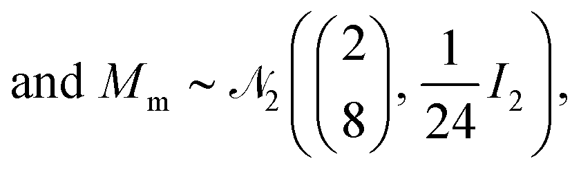 | (16) |
The R67 package rjags68 was used to compute the Bayesian inference of the augmented model. MCMC sampling algorithms were applied as implemented in the software JAGS 4.3.0.69
3 Results
The QMRA model (prior) and the augmented model were run at each month for which data were collected (May and September 2019 and each month from March to June 2021) (posteriors 1 to 6). For each model, two independent MCMC chains (using different initial values for the parameters) of 1![[thin space (1/6-em)]](https://www.rsc.org/images/entities/char_2009.gif) 400000 simulations with a burn-in period of 1000000 were run. Convergence of the MCMC run was assessed by graphical inspection of the chains.
400000 simulations with a burn-in period of 1000000 were run. Convergence of the MCMC run was assessed by graphical inspection of the chains.
In the following, the results and the update of prior beliefs in the model are described module by module.
3.1 Water contamination
The priors described in Table 1 yielded the following 95% credible intervals for water quality concentrations expressed here in log: kA ∈ [2; 6], kB ∈ [1; 5], kTP ∈ [6; 10], fLp ∈ [0.06, 0.14], log10(CA) ∈ [−0.4; 6.5], log10(CB) ∈ [0.6; 7.3], log10(CGT) ∈ [8; 12], log10(CWW) ∈ [13; 17], log10(CTP) ∈ [4; 10], log10(CLp,A) ∈ [−5; 1], log10(CLp,B) ∈ [−4; 2.5], and log10(CLp,GT) ∈ [3; 7]. These credible intervals are derived from the distributions described in Table 1 and the propagation of the uncertainty according to Fig. 5 for non-terminal variables (or parameters).
Fig. 6 and 7 illustrate that the groundwater (CLp,GT) and the water after treatment by the pilot A or B (CLp,A, CLp,B) show similar contamination levels (∼102 GC per L) indicating that the new irrigation process is as safe as the previous one (with groundwater without treatment). As expected, a significant log reduction between contamination of raw and treated wastewater for the posterior distributions appears (∼3log10 reduction). Nevertheless, one observes that the parameters kTP, kA and kB are smaller in the posterior distributions than in the prior distribution indicating that the data introduced at the CTP, CA and CB levels (see Fig. 5) are more contaminated than expected. This may be due to the storage of the water between treatments in large reservoirs or poor control of the treatment chain as discussed below.
 | ||
| Fig. 6 Prior (red) versus posterior marginal distributions of selected parameters and variables of the water contamination module of the augmented Bayesian network. Dashed lines represent the median of the prior marginal distributions. Distributions presented are in log10 (CFU per L). | ||
 | ||
| Fig. 7 Violin plots for concentrations of Legionella pneumophila (log10 GC per L). | ||
From the prior distributions (in red in Fig. 6) to the posterior ones, one observes reduced uncertainties (narrower distributions in posterior). The posterior distribution at June 2021 (in pink in Fig. 6) shows a reduction of the concentration after treatments: 1log10 reduction (from 106 to 105 GC per L) for the wastewater after treatment in the treatment plant and treatment A and similarly for treatment B. The transition to Legionella pneumophila from Legionella measurements analysed by PCR reduces again the contamination by 3log10.
Although a significant log reduction between raw and treated wastewater is observed, the differences between treatments A and B and groundwater are very slim compared to what would have been expected by the prior knowledge of processes A and B which should eliminate most of the bacteria. This may be due to storage issues or lack of control in the chain of experimentation and will be discussed in the following.
3.2 Air contamination
The air contamination module output is the concentration Cx,P (in GC per m3) of Legionella pneumophila in the air at distances x ∈ {100 m, 300 m, 500 m, 1000 m} from the source due to the irrigation using water of quality P ∈ {A, B, GT} (see Fig. 8). One observes reduced uncertainty from the prior to the posterior distributions of the concentration of Legionella pneumophila in the air for all treatments and distances. As expected, the distributions globally decrease with the distance: from 10−3 at 100 m to 10−5 at 1000 m for wastewater after treatment in TP and treatment A and similarly for treatment B and groundwater GT. The final predicted air concentrations are of similar intensity for irrigation using water from treatments A and B and groundwater which comforts the previous remarks on the quality of the proposed irrigation process. | ||
| Fig. 8 log10 of concentrations of Legionella pneumophila in the air due to the irrigation process for groundwater (GT), and after treatments A and B at 100 m and 1000 m from the source. | ||
3.3 Illness
Fig. 9 to 11 present the probabilities of clinical severity infection over one year, for farmers (see Fig. 9), for residents (see Fig. 10) and for passersby (see Fig. 11). For both clinical severity infections (csi) and others (inf), a decrease in the risk of contamination is observed with the distance for each category of people at risk: from 10−10 at 100 m to 10−13 at 1000 m for the risk of clinical severity infection for the farmers exposed to treatment A (and after treatment TP). A decay of approximately 1log10 is observed between farmers and residents for the probability of clinical severity infection (which is again the case between residents and passersby). Treatments A and B and groundwater give similar probabilities of infection with a slightly higher risk for groundwater which confirms the previous results that the new irrigation process is slightly safer than the one under use (with groundwater, without further treatment). It is also notable that the upper bound of the 95% credibility intervals never exceeds the US EPA annual infection benchmark70 of 10−4 infections per year (for drinking water) for clinical severity infections.
 | ||
| Fig. 9 log10 annual infection risks for L. pneumophila for the farmers due to sprinkler exposure at downwind distances ranging from 100 to 5000 meters from the source. The median (solid line) and interdecile confidence interval (dashed lines) are shown. Infection (Inf) or clinical severity infection (CSI) dose response model endpoints. | ||
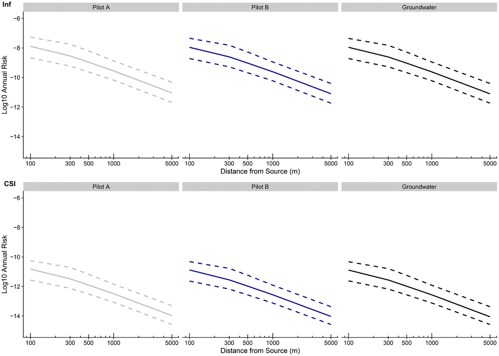 | ||
| Fig. 10 log10 annual infection risks for L. pneumophila for the residents due to sprinkler exposure at downwind distances ranging from 100 to 5000 meters from the source. The median (solid line) and interdecile confidence interval (dashed lines) are shown. Infection (Inf) or clinical severity infection (CSI) dose response model endpoints. | ||
 | ||
| Fig. 11 log10 annual infection risks for L. pneumophila for the passersby due to sprinkler exposure at downwind distances ranging from 100 to 5000 meters from the source. The median (solid line) and interdecile confidence interval (dashed lines) are shown. Infection (Inf) or clinical severity infection (CSI) dose response model endpoints. | ||
3.4 Scenario evaluation
Scenarios to determine how failures or very high initial contamination would affect the final risk were evaluated by computing the updated annual probabilities of infection with a new day of 10 simulated data as established by observed variables in the water contamination step of the model. In every scenario, all populations were tested as well as another toy population exposed 100% of the time of irrigation to the pathogen which could relate to children playing outside all irrigation days for instance. The results of all scenarios are presented in Fig. 12. | ||
| Fig. 12 log10 annual infection risks for L. pneumophila resulting from scenarios 1, 2 and 3. The red dotted line represents the US EPA threshold of −4log annual probability of infection. Toy population and farmers are represented from left to right on the first line and residents and passersby on the second line. | ||
(15, 1) as a classical contamination as established by expert knowledge and literature data (see Table 1), log10(CTP,i) (i = 1, …, 10) data were obtained with a decay of around 8log of log10(CWW,i) as the WWTP standard treatment is supposed to be effective (see Table 1, kTP ∼ (8, 1) as established by expert knowledge and literature data when the WWTP standard treatment is effective) and finally, log10(CA,i) (i = 1, …,10) data were obtained with around no log decay (kA ∼ (0, 1)) because in this scenario, a failure of the experimental pilot A is supposed. The annual probability of infection increased by 0.8log which gave a median of −4.89log and an interdecile range of 1.33log at 100 m for the toy population. For all distances and all populations studied, the 9th decile never exceeded the US EPA threshold of −4log annual probability of infection.
(20, 1) to simulate high contamination of the source and that the pilot treatment is supposed to be effective (see Table 1, kA ∼ (4, 1) as established by expert knowledge and literature data when the WWTP standard treatment is effective). This resulted in an increase of 0.9log of the annual probability of infection which is comparable to the previous scenario. Once more, the 9th decile never exceeds the US EPA threshold for annual probability of infection but gets even closer with a value of −4.2log at 100 m for the toy population.
log. This threshold was exceeded by the median for the toy population for 100 m with a value of −3.79 and by the 9th decile at 300 m with a value of −3.20. The risk for the other populations did not exceed this threshold with a maximum value of −4.88 attained for farmers at 100 m from the source.
4 Discussion
A general Bayesian network methodology was applied to a QMRA problematic to monitor the risk of Legionella infection in the vicinity of agricultural plots irrigated with two experimental water treatment pilots. The general Bayesian network approach allows for simple accounting for variability and uncertainty in the context of complex modelling such as QMRA models. In the developed approach, a modified Gaussian plume dispersion model was used to compute health risks according to different scenarios, using knowledge of meteorological conditions over long periods (>20 years here) and distinguishing three categories of persons at risk, two dose–response endpoints and different downwind distances from the sprinkler.The general Bayesian network methodology used is a very powerful approach without any discretization to quantify complex phenomena in presence of prior knowledge and scarce data. Indeed, the approach allows taking into account expert knowledge and literature data in the prior distributions of the random variables and consideration of simultaneously collected data all over the phenomenon. The uncertainty and variability of each variable are evaluated through the strength of its prior knowledge combined with the strength of the data information provided by the size of data sets, which is not the case in simulated networks, just using Monte Carlo simulations, where the data are fitted marginally to establish the prior distributions, and then their provided uncertainty is spread poorly in the whole network. Also, by contrast with non-parametric Bayesian networks, in the highly parametric approach used in this paper, the knowledge of the functional relationships between the random variables is maximized to permit the estimation of quantities of interest in the context of scarce data.
Both for annual infection and clinical severity infection, no major difference was observed between risks induced by irrigation using water treated by treatment A (ultrafine filtration, after standard treatment plant), treatment B (UV, after standard treatment plant) and groundwater. This comforts the prior belief that treatments A and B give a water quality at least comparable to the quality of the groundwater. Risks were observed to decrease with distance from the source, which was expected according to the atmospheric dispersion modelling. An approximately 1log difference was observed between each of the studied categories of people (farmers, residents and passersby), with the passersby being the population least at risk and farmers the population most at risk according to the model (logical order according to the exposure time).
High values of Legionella in GC per L were found in the different analyzed compartments even after the two studied treatments. The impact of the storage time in large reservoirs after the two pilots can in part explain some high observed levels. The cleaning of these tank covers appears as an important point to check for operational applications. Such an observation reveals the interest of working in the first steps with GC for an operational monitoring of the water quality; GC are uncensored data and PCR analyses are less time consuming and can be done routinely. The values reported in GC were first introduced in the model until the risk characterization, and then converted in CFU applying a significant decrease of 10 × 103 between GC and UFC, as quantified from the laboratory analytical results and as often observed in the literature. Let us mention that if one applies this decrease factor (fCFU) on the contamination after the tertiary treatment A and B, i.e. on CA and CB, the two treatments are class A reclaimed water because only 0.1% are above the new European limit (<1000 CFU L−1).
Note that the US EPA criterion of annual probability of infection was used throughout the study instead of disability adjusted life years (DALYs) recommended by the WHO. Indeed, the current method of estimation of the DALY for Legionella pneumophila is still controversial to our knowledge. The DALY can be computed as 0.97 times the annual probability of infection with low precision71 and a recent study72 taking the heterogeneity of responses to contamination into account could be used to derive a better estimation of the DALY.
It is notable that the upper bound of the interdecile credibility intervals of the posterior never exceeded the target risk values for infection (10−4 annual probability of infection for the US EPA criterion and 10−6 disability adjusted life year per person per year, i.e. DALY pppy for the WHO criterion). However, a slow decrease of risk is observed with the distance to the source which is the consequence of the meteorological conditions in the vicinity of the agricultural plots. This observation is consistent with previous studies that have predicted the long-range transport of Legionella.19,22,73 In the local climatic context of Tarbes where the decrease is slow, it seems essential that the concentration has to be already low (below 104) at 100 m from the sprinklers.
The developed tool is ready to be updated especially by air measured concentrations on the plots by the irrigations with reclaimed water that will take place starting in Summer 2021. This tool will then be used to monitor the potential risks in the vicinity of the experimental plots and thus meet the public health demands of population protection.
In a more general QMRA context, the proposed model gives an operational tool and theoretically stable methodology to maintain a continuous monitoring of the risks induced by the irrigation practices on the agricultural plots under study. This methodology can adapt to new sets of data and easily update the model if given new information. This model can easily be adapted to other well-known pathogens through the enlightened adaptation of a few priors such as the ones on the decay parameter λ, the dose–response parameter r, etc.
A challenge would lie in the usage of the model to answer simultaneous multipathogen risk analysis. Also, one of the next main interests lies in the addition of modelisation of the impact of the irrigation with reclaimed wastewater on the quality of the groundwater to simultaneously quantify the inhalation induced risk and the groundwater table contamination by reclaimed wastewater transport in soil. Furthermore, it could be very interesting to link the final probability of infection over the year to epidemiological data over the region as done by Albert et al. (2008),36 linking an epidemiological study of campylobacteriosis cases to the probability of suffering from campylobacteriosis over one year in France due to broiler meat. In the same spirit, the link would necessitate here the introduction of a random variable for the water reuse attributable fraction of Legionella infection to take other routes of contaminations into account. Also, it would necessitate considering only a fraction of the cases that could be due to this irrigation zone. But for the moment, the epidemiological data at disposal are only available at a large geographical scale (the surface of the Occitanie region is approximately 70000 km2 compared to the surface of the study zone which is approximately 6 km2) and it does not seem reasonable to link these data to the very local modeling proposed.
5 Conclusions
• A general Bayesian network as an operational tool to maintain the monitoring of the risks induced by a water reuse irrigation practice.• The first developed general Bayesian network approach in QMRA for wastewater surveillance. The main asset is that risks are quantified with their uncertainties at each desired time taking into account new and past data.
• The QMRA model describes the exposure pathway of the water contamination from the entrance of the WWTP to the infection risk using pathogen decay models in the WWTP, a Gaussian plume model for the air contamination, an inhalation model for the population exposure and finally a dose–response model for risk characterization.
• The uncertainty of the probabilistic QMRA model is reduced by the introduction of observed data (pathogen concentrations and regional meteorological data) along the modelisation to obtain the distribution of the number of pathogens before and after treatment in the WWTP, the number of aerosolised pathogens, and the concentration of pathogens in the air at different distances, and finally the exposure and illness distributions for three different categories of population at risk and two illness endpoints.
• Legionella annual subclinical infection risk and annual clinical severity infection risk linked to the agricultural irrigation using the groundwater table or two experimental water treatment pilots are inferred to be below the 10−4 tolerable limit defined by the US EPA for farmers, passersby and residents at distances between 100 m and 1000 m away from sprinklers.
• Such a dynamic approach can be applied to various pathogens in the context of wastewater reuse.
Conflicts of interest
There are no conflicts to declare.Acknowledgements
The partners of the project are Polymem, Bio-UV, Ecofilae, VERI, Veolia Eau, Sede, and Inrae-Transfert Narbonne. Established with the authorization of the Tarbes-Lourdes-Pyrénées Syndicate, owner of the treatment plant, this project involves farmers as well as the Departmental Federation of Farmers' Unions of Hautes-Pyrénées (FDSEA 65) and the Chamber of farming Hautes-Pyrénées. The project is FUI funded, and co-funded by the Sud-West region and Occitania region (France).Notes and references
- P. T. Vo, H. H. Ngo, W. Guo, J. L. Zhou, P. D. Nguyen and A. Listowski, et al., A mini-review on the impacts of climate change on wastewater reclamation and reuse, Sci. Total Environ., 2014, 494–495, 9–17 CAS , Available from: https://www.sciencedirect.com/science/article/pii/S0048969714009632.
- H. Elbasiouny, H. El-Ramady and F. Elbehiry, Sustainable and Green Management of Wastewater Under Climate Change Conditions, The Handbook of Environmental Chemistry, 2021, pp. 1–19, Available from: DOI:10.1007/698_2021_787.
- J. S. Guest, S. J. Skerlos, J. L. Barnard, M. B. Beck, G. T. Daigger and H. Hilger, et al., A New Planning and Design Paradigm to Achieve Sustainable Resource Recovery from Wastewater, Environ. Sci. Technol., 2009, 43(16), 6126–6130, DOI:10.1021/es9010515.
- J. Fito and S. W. Van Hulle, Wastewater reclamation and reuse potentials in agriculture: towards environmental sustainability, Environ. Dev. Sustain., 2021, 23(3), 2949–2972 CrossRef.
- J. Hristov, J. Barreiro-Hurle, G. Salputra, M. Blanco and P. Witzke, Reuse of treated water in European agriculture: Potential to address water scarcity under climate change, Agric. Water Manag., 2021, 251, 106872 CrossRef PubMed , Available from: https://www.sciencedirect.com/science/article/pii/S0378377421001372.
- EP. Water Reuse - Setting Minimum Requirements, European Parliament, 2020 Search PubMed.
- Food and Agriculture Organization of the United Nations, The state of the world's land and water resources for food and agriculture: Managing systems at risk, Earthscan, 2011 Search PubMed.
- A. A. Adegoke, I. D. Amoah, T. A. Stenström, M. E. Verbyla and J. R. Mihelcic, Epidemiological evidence and health risks associated with agricultural reuse of partially treated and untreated wastewater: a review, Front. Public Health, 2018, 6, 337 CrossRef PubMed.
- J. Bartram, Y. Chartier, J. V. Lee, K. Pond and S. Surman-Lee, Legionella and the prevention of legionellosis, World Health Organization, 2007 Search PubMed.
- Organization WH, WHO. Guidelines for drinking-water quality, World Health Organization, 2004, vol. 1 Search PubMed.
- Organization WH, Guidelines for safe recreational water environment, World Health Organization, 2006, vol. 1 Search PubMed.
- Organization WH, et al., WHO guide to ship sanitation, World Health Organization, 2011 Search PubMed.
- EC. Water Reuse, European Commission, 2021 Search PubMed.
- D. Courault, I. Albert, S. Perelle, A. Fraisse, P. Renault and A. Salemkour, et al., Assessment and risk modeling of airborne enteric viruses emitted from wastewater reused for irrigation, Sci. Total Environ., 2017, 592, 512–526 CrossRef CAS PubMed.
- T. Paez-Rubio, E. Viau, S. Romero-Hernandez and J. Peccia, Source bioaerosol concentration and rRNA gene-based identification of microorganisms aerosolized at a flood irrigation wastewater reuse site, Appl. Environ. Microbiol., 2005, 71(2), 804–810 CrossRef CAS PubMed.
- B. Teltsch and E. Katzenelson, Airborne enteric bacteria and viruses from spray irrigation with wastewater, Appl. Environ. Microbiol., 1978, 35(2), 290–296 CrossRef CAS PubMed.
- ANSES, Avis et rapport d'expertise : Réutilisation des eaux usées traitées pour l'irrigation des cultures, l'arrosage des espaces verts par aspersion et le lavage des voiries, Saisine n°2009-SA-0329, 2012 Search PubMed.
- M. Blanky, Y. Sharaby, S. Rodríguez-Martínez, M. Halpern and E. Friedler, Greywater reuse - Assessment of the health risk induced by Legionella pneumophila, Water Res., 2017, 125, 410–417 CrossRef CAS PubMed , Available from: https://www.sciencedirect.com/science/article/pii/S0043135417307212.
- K. A. Hamilton, M. T. Hamilton, W. Johnson, P. Jjemba, Z. Bukhari and M. LeChevallier, et al., Health risks from exposure to Legionella in reclaimed water aerosols: Toilet flushing, spray irrigation, and cooling towers, Water Res., 2018, 134, 261–279 CrossRef CAS PubMed , Available from: https://www.sciencedirect.com/science/article/pii/S0043135417310175.
- K. A. Hamilton and C. N. Haas, Critical review of mathematical approaches for quantitative microbial risk assessment (QMRA) of Legionella in engineered water systems: research gaps and a new framework, Environ. Sci.: Water Res. Technol., 2016, 2, 599–613 RSC.
- B. Diederen, Legionella spp. and Legionnaires' disease, J. Infect., 2008, 56(1), 1–12 CrossRef CAS PubMed.
- S. M. Walser, D. G. Gerstner, B. Brenner, C. Höller, B. Liebl and C. E. Herr, Assessing the environmental health relevance of cooling towers–a systematic review of legionellosis outbreaks, Int. J. Hyg. Environ. Health, 2014, 217(2–3), 145–154 CrossRef PubMed.
- P. Xu, C. Zhang, X. Mou and X. C. Wang, Bioaerosol in a typical municipal wastewater treatment plant: concentration, size distribution, and health risk assessment, Water Sci. Technol., 2020, 82, 1547–1559 CrossRef PubMed.
- A. D. Loenenbach, C. Beulens, S. M. Euser, J. P. van Leuken, B. Bom and W. van der Hoek, et al., Two community clusters of Legionnaires' Disease directly linked to a biologic wastewater treatment plant, the Netherlands, Emerging Infect. Dis., 2018, 24(10), 1914 CrossRef PubMed.
- J. W. Tang, The effect of environmental parameters on the survival of airborne infectious agents, J. R. Soc., Interface, 2009, 6(suppl_6), S737–S746 Search PubMed.
- C. N. Haas, J. B. Rose and C. P. Gerba, Quantitative microbial risk assessment, John Wiley & Sons, 2014 Search PubMed.
- D. P. Janevska, R. Gospavic, E. Pacholewicz and V. Popov, Application of a HACCP–QMRA approach for managing the impact of climate change on food quality and safety, Food Res. Int., 2010, 43(7), 1915–1924 CrossRef , Available from: https://www.sciencedirect.com/science/article/pii/S0963996910000438.
- S. Petterson and N. Ashbolt, QMRA and water safety management: review of application in drinking water systems, J. Water Health, 2016, 14(4), 571–589 CrossRef CAS PubMed.
- C. E. L. Owens, M. L. Angles, P. T. Cox, P. M. Byleveld, N. J. Osborne and M. B. Rahman, Implementation of quantitative microbial risk assessment (QMRA) for public drinking water supplies: Systematic review, Water Res., 2020, 174, 115614 CrossRef CAS PubMed , Available from: https://www.sciencedirect.com/science/article/pii/S0043135420301500.
- D. Mara, P. Sleigh, U. Blumenthal and R. Carr, Health risks in wastewater irrigation: comparing estimates from quantitative microbial risk analyses and epidemiological studies, J. Water Health, 2007, 5(1), 39–50 CrossRef CAS PubMed.
- R. Wang, X. Li and C. Yan, Seasonal fluctuation of aerosolization ratio of bioaerosols and quantitative microbial risk assessment in a wastewater treatment plant, Environ. Sci. Pollut. Res., 2021, 1–18 Search PubMed.
- A. Simhon, V. Pileggi, C. A. Flemming, G. Lai and M. Manoharan, Norovirus risk at a golf course irrigated with reclaimed water: Should QMRA doses be adjusted for infectiousness?, Water Res., 2020, 183, 116121 CrossRef CAS PubMed.
- A. Carducci, G. Donzelli, L. Cioni and M. Verani, Quantitative microbial risk assessment in occupational settings applied to the airborne human adenovirus infection, Int. J. Environ. Res. Public Health, 2016, 13(7), 733 CrossRef PubMed.
- C. Yan, Z. Gui and J. Wu, Quantitative microbial risk assessment of bioaerosols in a wastewater treatment plant by using two aeration modes, Environ. Sci. Pollut. Res., 2021, 28(7), 8140–8150 CrossRef CAS.
- V. Zhiteneva, U. Hübner, G. J. Medema and J. E. Drewes, Trends in conducting quantitative microbial risk assessments for water reuse systems: A review, Microb. Risk Anal., 2020, 16, 100132 CrossRef , Available from: https://www.sciencedirect.com/science/article/pii/S2352352220300384.
- I. Albert, E. Grenier, J. B. Denis and J. Rousseau, Quantitative risk assessment from farm to fork and beyond: A global Bayesian approach concerning food-borne diseases, Risk Anal., 2008, 28(2), 557–571 CrossRef PubMed.
- J. Smid, D. Verloo, G. Barker and A. Havelaar, Strengths and weaknesses of Monte Carlo simulation models and Bayesian belief networks in microbial risk assessment, Int. J. Food Microbiol., 2010, 139, S57–S63 CrossRef PubMed.
- T. D. Nielsen and F. V. Jensen, Bayesian networks and decision graphs, Springer Science & Business Media, 2009 Search PubMed.
- M. Scutari and J. B. Denis, Bayesian Networks: With Examples in R, Chapman and Hall/CRC, 2nd edn, 2022 Search PubMed.
- C. Rigaux, S. Ancelet, F. Carlin, C. Nguyen-thé and I. Albert, Inferring an augmented Bayesian network to confront a complex quantitative microbial risk assessment model with durability studies: application to Bacillus cereus on a courgette purée production chain, Risk Anal., 2013, 33(5), 877–892 CrossRef.
- D. Beaudequin, F. Harden, A. Roiko and K. Mengersen, Utility of Bayesian networks in QMRA-based evaluation of risk reduction options for recycled water, Sci. Total Environ., 2016, 541, 1393–1409 CrossRef CAS , Available from: https://www.sciencedirect.com/science/article/pii/S0048969715308469.
- D. Beaudequin, F. Harden, A. Roiko, H. Stratton, C. Lemckert and K. Mengersen, Modelling microbial health risk of wastewater reuse: A systems perspective, Environ. Int., 2015, 84, 131–141 CrossRef.
- P. A. Aguilera, A. Fernández, R. Fernández, R. Rumí and A. Salmerón, Bayesian networks in environmental modelling, Environ. Model. Softw., 2011, 26(12), 1376–1388 CrossRef.
- K. B. Korb and A. E. Nicholson, Bayesian artificial intelligence, CRC press, 2010 Search PubMed.
- D. Beaudequin, F. Harden, A. Roiko, H. Stratton, C. Lemckert and K. Mengersen, Beyond QMRA: Modelling microbial health risk as a complex system using Bayesian networks, Environ. Int., 2015, 80, 8–18 CrossRef PubMed , Available from: https://www.sciencedirect.com/science/article/pii/S0160412015000719.
- D. Beaudequin, F. Harden, A. Roiko and K. Mengersen, Potential of Bayesian networks for adaptive management in water recycling, Environ. Model. Softw., 2017, 91, 251–270 CrossRef , Available from: https://www.sciencedirect.com/science/article/pii/S1364815217300919.
- J. Herrera-Murillo, D. Mora-Campos, P. Salas-Jimenez, M. Hidalgo-Gutierrez, T. Soto-Murillo and J. Vargas-Calderon, et al., Wastewater Discharge and Reuse Regulation in Costa Rica: An Opportunity for Improvement, Water, 2021, 13(19), 2631 CrossRef.
- V. Zhiteneva, G. Carvajal, O. Shehata, U. Hübner and J. E. Drewes, Quantitative microbial risk assessment of a non-membrane based indirect potable water reuse system using Bayesian networks, Sci. Total Environ., 2021, 780, 146462 CrossRef CAS PubMed , Available from: https://www.sciencedirect.com/science/article/pii/S0048969721015308.
- R. Pouillot, I. Albert, M. Cornu and J. Denis, Estimation of uncertainty and variability in bacterial growth using Bayesian inference. Application to Listeria monocytogenes, Int. J. Food Microbiol., 2003, 81(2), 87–104 CrossRef PubMed.
- S. Højsgaard, Graphical independence networks with the gRain package for R, J. Stat. Softw., 2012, 46(10), 1–26 Search PubMed.
- I. Albert, E. Espié, H. de Valk and J. B. Denis, A Bayesian evidence synthesis for estimating campylobacteriosis prevalence, Risk Anal., 2011, 31(7), 1141–1155 CrossRef PubMed.
- W. R. Gilks, S. Richardson and D. Spiegelhalter, Markov Chain Monte Carlo in Practice, Chapman & Hall/CRC Interdisciplinary Statistics, Taylor & Francis, 1995 Search PubMed.
- M. E. Verbyla, E. M. Symonds, R. C. Kafle, M. R. Cairns, M. Iriarte and A. Mercado Guzman, et al., Managing microbial risks from indirect wastewater reuse for irrigation in urbanizing watersheds, Environ. Sci. Technol., 2016, 50(13), 6803–6813 CrossRef CAS PubMed.
- M. Palusińska-Szysz and M. Cendrowska-Pinkosz, Pathogenicity of the family Legionellaceae, Arch. Immunol. Ther. Exp., 2009, 57(4), 279–290 CrossRef.
- N. P. Cianciotto, Pathogenicity of Legionella pneumophila, Int. J. Med. Microbiol., 2001, 291(5), 331–343 CrossRef CAS PubMed.
- J. H. Seinfeld and S. N. Pandis, Atmospheric chemistry and physics: from air pollution to climate change, John Wiley & Sons, 2016 Search PubMed.
- US EPA, Exposure Handbook, US Environmental Protection Agency, 2011 Search PubMed.
- T. W. Armstrong and C. N. Haas, A Quantitative Microbial Risk Assessment Model for Legionnaires' Disease: Animal Model Selection and Dose-Response Modeling, Risk Anal., 2007, 27(6), 1581–1596, DOI:10.1111/j.1539-6924.2007.00990.x.
- B. Molle, L. Huet, S. Tomas, J. M. Granier, P. Dimaiolo and C. Rosa, Caractérisation du risque de dérive et d'évaporation d'une gamme d'asperseurs d'irrigation. Application à la définition des limites d'utilisation de l'aspersion en réutilisation d'eaux usées traitées, Ph.D. thesis, Irstea, 2009 Search PubMed.
- T. Paez-Rubio, A. Ramarui, J. Sommer, H. Xin, J. Anderson and J. Peccia, Emission rates and characterization of aerosols produced during the spreading of dewatered class B biosolids, Environ. Sci. Technol., 2007, 41(10), 3537–3544 CrossRef CAS PubMed.
- P. Hambleton, M. Broster, P. Dennis, R. Henstridge, R. Fitzgeorge and J. Conlan, Survival of virulent Legionella pneumophila in aerosols, Epidemiol. Infect., 1983, 90(3), 451–460 CAS.
- P. Dennis and J. Lee, Differences in aerosol survival between pathogenic and non-pathogenic strains of Legionella pneumophila serogroup 1, J. Appl. Bacteriol., 1988, 65(2), 135–141 CrossRef CAS PubMed.
- P. Stellacci, L. Liberti, M. Notarnicola and C. N. Haas, Hygienic sustainability of site location of wastewater treatment plants: A case study, I. Estimating odour emission impact, Desalination, 2010, 253(1–3), 51–56 CrossRef CAS.
- J. P. Brooks, M. R. McLaughlin, C. P. Gerba and I. L. Pepper, Land application of manure and class B biosolids: An occupational and public quantitative microbial risk assessment, J. Environ. Qual., 2012, 41(6), 2009–2023 CrossRef CAS PubMed.
- D. Muller, M. L. Edwards and D. W. Smith, Changes in iron and transferrin levels and body temperature in experimental airborne legionellosis, J. Infect. Dis., 1983, 147(2), 302–307 CrossRef CAS.
- R. Fitzgeorge, A. Baskerville, M. Broster, P. Hambleton and P. Dennis, Aerosol infection of animals with strains of Legionella pneumophila of different virulence: comparison with intraperitoneal and intranasal routes of infection, Epidemiol. Infect., 1983, 90(1), 81–89 CAS.
- R Core Team, R: A Language and Environment for Statistical Computing, Vienna, Austria, 2020, Available from: https://www.R-project.org/ Search PubMed.
- M. Plummer, rjags: Bayesian Graphical Models using MCMC, 2019, R package version 4-10. Available from: https://CRAN.R-project.org/package=rjags.
- M. Plummer, JAGS: A program for analysis of Bayesian graphical models using Gibbs sampling, in Proceedings of the 3rd international workshop on distributed statistical computing, Vienna, Austria, 2003, vol. 124, pp. 1–10 Search PubMed.
- EPA U, Potable reuse compendium. EPA 810-R-17–002 2017, Office of Ground Water and Drinking Water, Washington, 2017 Search PubMed.
- K. A. Hamilton, M. T. Hamilton, W. Johnson, P. Jjemba, Z. Bukhari and M. LeChevallier, Risk-Based Critical Concentrations of Legionella pneumophila for Indoor Residential Water Uses, Environ. Sci. Technol., 2019, 53(8), 4528–4541, DOI:10.1021/acs.est.8b03000.
- M. H. Weir, A. L. Mraz and J. Mitchell, An Advanced Risk Modeling Method to Estimate Legionellosis Risks Within a Diverse Population, Water, 2020, 12(1), 43 CrossRef , Available from: https://www.mdpi.com/2073-4441/12/1/43.
- K. Borgen, I. Aaberge, Ø. Werner-Johansen, K. Gjøsund, B. Størsrud and S. Haugsten, et al., A cluster of Legionnaires' disease linked to an industrial plant in southeast Norway, June-July 2008, Eurosurveillance, 2008, 13(38), 18985 CrossRef PubMed.
Footnotes |
| † Electronic supplementary information (ESI) available. See DOI: https://doi.org/10.1039/d2ew00311b |
| ‡ https://www.santepubliquefrance.fr/maladies-et-traumatismes/maladies-et-infections-respiratoires/legionellose (accessed on October 4th 2022). |
| § https://www.smartfertireuse.fr/les-moyens (accessed on October 4th 2022). |
| ¶ https://tinyurl.com/5n6v4y38 (accessed on October 4th 2022). |
| This journal is © The Royal Society of Chemistry 2023 |