
 Open Access Article
 This Open Access Article is licensed under a
 Creative Commons Attribution 3.0 Unported Licence
Luminescent solar concentrators for building integrated photovoltaics: opportunities and challenges†
Bryce S.
Richards
 *ab and
Ian A.
Howard
ab
*ab and
Ian A.
Howard
ab
aInstitute of Microstructure Technology, Karlsruhe Institute of Technology, Hermann-von-Helmholtz-Platz 1, 76344, Eggenstein-Leopoldshafen, Germany. E-mail: bryce.richards@kit.edu
bLight Technology Institute, Karlsruhe Institute of Technology, Engesserstrasse 13, 76131 Karlsruhe, Germany
First published on 7th July 2023
Abstract
This review examines the application of luminescent solar concentrators (LSCs) for building integrated photovoltaics (BIPV), both in terms of opaque façade elements and as semi-transparent windows. Many luminophores have been developed for LSC applications, and their efficiencies examined in lab-scale (<25 cm2) devices. This analytical review illustrates, using ray-tracing simulations, the technical challenges to maintaining efficiency when scaling these energy conversion devices to pilot- (1000 cm2) and commercial-scale (100![[thin space (1/6-em)]](https://www.rsc.org/images/entities/char_2009.gif) 000 cm2) modules. Based on these considerations, ambitious but feasible target efficiencies for LSCs based on ideal quantum dot (QD) luminophores are suggested as follows – for opaque and semi-transparent (50% average visible transmission), respectively: (i) 11.0% and 5.5% for lab-scale devices; (ii) 10.0% and 5.0% for pilot-scale modules; and (iii) 9.0% and 4.5% for commercial-scale modules. It is worth noting though, that the QD design requirements – particularly with regard to the overlap integral between the absorption and emission spectrum – become very critical as the LSC area increases. Whereas it is difficult to see opaque LSCs successfully competing against standard flat-plate photovoltaic modules for building integration, the application of semi-transparent LSCs as power-generating window elements has potential. Therefore, an economic analysis of the inclusion of LSCs into commercial glazing elements is presented and the potential for novel technologies – such as down-conversion (quantum-cutting) and controlling the direction of emitted light – to move this technology towards application is also discussed.
000 cm2) modules. Based on these considerations, ambitious but feasible target efficiencies for LSCs based on ideal quantum dot (QD) luminophores are suggested as follows – for opaque and semi-transparent (50% average visible transmission), respectively: (i) 11.0% and 5.5% for lab-scale devices; (ii) 10.0% and 5.0% for pilot-scale modules; and (iii) 9.0% and 4.5% for commercial-scale modules. It is worth noting though, that the QD design requirements – particularly with regard to the overlap integral between the absorption and emission spectrum – become very critical as the LSC area increases. Whereas it is difficult to see opaque LSCs successfully competing against standard flat-plate photovoltaic modules for building integration, the application of semi-transparent LSCs as power-generating window elements has potential. Therefore, an economic analysis of the inclusion of LSCs into commercial glazing elements is presented and the potential for novel technologies – such as down-conversion (quantum-cutting) and controlling the direction of emitted light – to move this technology towards application is also discussed.
Broader contextThere is significant drive within Europe to promote zero-energy buildings, such that they counterbalance their energy consumption with on-site renewable energy generation. To realise zero-energy office buildings, a semi-transparent energy conversion technology for their large glass facades is highly desirable, while still allowing for 50% visible light transmission. Luminescent solar concentrators (LSCs) could be such a technology. Based on large-area, semi-transparent “window” waveguides with thin strips of solar cells hidden at their edges (in the window framing), LSCs allow for variations in shape, colour, and form as well as trading-off the amount of electricity produced compared to the amount of daylight transmitted. This review sets out the challenges and requirements to maintain efficiencies measured on 25 cm2 laboratory-scale test devices when moving to 100000 cm2 sizes needed for true commercial application. In an optimistic but feasible scenario, it should be possible to maintain 75% of the small lab-scale efficiency in this scale-up process; this would lead to a 4.5% power conversion efficiency of a commercial-scale module with 50% transmission of visible light. Cost estimates are also presented, which will also play a decisive role in determining the commercial fate of this technology.
|
1. Introduction
Buildings in European cities contribute 36% of greenhouse gas emissions.1 To meet Europe's target in the Paris Agreement, these emissions must be reduced by 80% before 2050. The EU Energy Performance of Buildings Directive has required since 2020 that all new-builds be near zero energy buildings,2 and it is proposed that all new-builds must be zero energy by 2030.3 Today, solar power generated from photovoltaics (PV) is one of the cheapest energy sources within Europe. Being a modular technology with no moving parts, PV lends itself well to use as a construction element, for example in the roofs and façades of buildings. This application is known as building integrated photovoltaics (BIPV). The BIPV market is expected to grow by US$10 billion over the next five years, representing a compound annual growth rate of 17%, with commercial buildings making up the largest share.4BIPV technologies that are competing for a portion of the glass façade market include classical crystalline silicon (c-Si) solar cells that are spaced to allow for daylighting, and thin-film PV technologies modified to achieve some transparency, as summarised by Kuhn et al.5 While flat-plate PV technologies currently dominate in all sectors including BIPV, the large size of glass sheets required for the BIPV industry (e.g., up to 10 m2 for curtain wall elements) are well beyond the size of a typical large PV module today (1–2 m2). This limits the number of capable manufacturers world-wide to just a handful. Also, some architects6 and PV companies (e.g. discussed by Xiang et al.7) place a great importance in moving away from the standard dark blue or black module colour when it comes to BIPV applications. Finally, sometimes having a form that is not flat and rectangular is desirable for the architect of a building.
For such BIPV applications, luminescent solar concentrators (LSC) have long been proposed as an ideal solution, having been initially developed in the mid-1970s.8,9 Although the LSC concept was originally developed as a novel way of concentrating sunlight onto strips of solar cells mounted on the edge of the LSC, it has been explored with respect to a wide range of applications: daylighting;10 indoor PV;11 smart windows;12 noise barriers;13 a modern rendition of stained-glass windows14 and artwork;15,16 luminescent greenhouses;17 solar lasers;18 photochemistry;19 enhanced algal growth;20 thermal energy conversion;21 and for free-space optical communication systems.22 Many of these applications are summarised in recent reviews,23–25 while other works have focused on establishing the theoretical upper limit of the conversion efficiency of a LSC.26 This review focuses on evaluating the performance and challenges of LSCs when combined with edge-coupled solar cells, particularly looking towards larger-area elements that could be used for BIPV. In particular, the goal is to determine what challenging-but-realistic efficiency targets the LSC technology needs to meet and if the projected LSC module costs are compatible with BIPV applications. These are considered for both opaque façade modules and semi-transparent glazing elements.
An overview of the operating principle of a LSC is illustrated in Fig. 1. Sunlight (①) is incident on the top surface of the LSC, the main component of which is a sheet fabricated using a transparent material with a refractive index, typically n ∼ 1.5 that will act as a waveguide for the luminescence. A fraction of the incident light is lost to reflectance (②) and transmittance (③), although the latter is also desired for the semi-transparent window applications. A significant fraction of light is absorbed by the luminescent centres embedded in the sheet (④), which in this work are assumed to be semiconducting quantum dots (QDs). The probability of luminescence being emitted by the QDs is given by the PLQY. Assuming isotropic emission of the luminescence, a significant fraction of this will ideally be ⑤ transported via total internal reflection (TIR) to ⑥ the perimeter of the LSC. Along the edges of the LSC, ⑦ long, narrow strips of crystalline silicon (c-Si) solar cells are mounted, attached using an adhesive or encapsulant. The critical angle (θc) in a waveguide with nhost = 1.5 is 41.8°, which means that ⑧ any luminescence emitted at a smaller angle is lost from the front or rear surface. These are called escape cone losses. In addition, there is often ⑨ an overlap between the absorption and emission spectra. This results in a fraction of the luminescence being reabsorbed, which is followed by re-emission event with the same PLQY, escape cone losses (ECL), and chance of subsequent reabsorption. Also, not all of the trapped luminescence reaches the edges of the LSC due to  the parasitic absorption and scattering of the host.
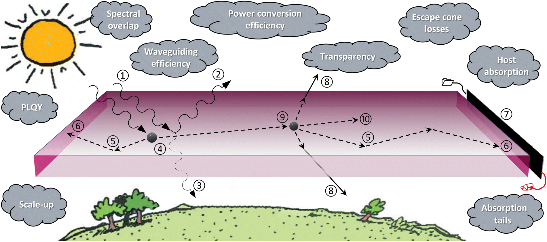 | ||
Fig. 1 Overview of the luminescent solar concentrator (LSC) technology demonstrating the working principle, step-by-step: ① sunlight is incident on the front surface of the LSC; with a fraction of this being lost to ② reflectance (defined by the Fresnel equations) and ③ transmittance; a significant fraction of light is ④ absorbed by the luminescent centres – in this case semiconducting quantum dots (QD) – which emit with a certain photoluminescence quantum yield (PLQY); ideally ⑤ the luminescence is transported via total internal reflection (TIR) to ⑥ the edges of the LSC where ⑦ long, narrow strips of crystalline silicon (c-Si) solar cells are attached to all edges via an encapsulant (not shown) that convert the luminescence into DC electricity. ⑧ A sizable fraction is not trapped and departs via both the front and rear surfaces (escape cones defined by the critical angle); additionally, ⑨ due to overlapping absorption and emission spectra, some luminescence may be reabsorbed by a neighbouring QD; while  losses are also induced by the parasitic absorption of the host. In this schematic, any scattering of light from within the bulk and/or at surfaces is not considered. Around the perimeter of the diagram, the key challenges for the LSC technology are highlighted, including: escape cone losses, PLQY, spectral overlap, waveguiding efficiency, absorption tails, parasitic host absorption and scattering, the overall power conversion efficiency, as well as issues relating to the degree of transparency of the LSC and scaling-up to the m2-scale. losses are also induced by the parasitic absorption of the host. In this schematic, any scattering of light from within the bulk and/or at surfaces is not considered. Around the perimeter of the diagram, the key challenges for the LSC technology are highlighted, including: escape cone losses, PLQY, spectral overlap, waveguiding efficiency, absorption tails, parasitic host absorption and scattering, the overall power conversion efficiency, as well as issues relating to the degree of transparency of the LSC and scaling-up to the m2-scale. | ||
There are several unique features of the LSC technology, which are discussed here. Firstly, in contrast to classical highly-concentrating (300–1000×) CPV systems that require precise tracking of the path of the sun – to within 0.5° accuracy27 – throughout the day, the LSC one of the only solar technologies able to concentrate not only direct rays of sunlight, but also diffuse light.28,29 This is important in cloudier environments such as in central Europe, were 50–60% of solar irradiance is diffuse.30 Secondly, the LSC concentration ratio is limited in theory only by the ratio of the top surface area to that of the perimeter, although it was recognised early on that the Stokes shift (referred to in this work as the overlap integral between the absorption and emission spectra) was a critical parameter that limited the concentration ratio in practice.8,28,29,31 Thirdly, if the wavelengths of the luminescence that are incident upon the solar cell are matched to the bandgap then the excess energy generated in the solar cell with each absorbed photon is small. This reduces lattice thermalisation losses with respect to normal solar illumination of the solar cell, and therefore results in less heat generation within the solar cells.32 Such operation under ‘cool light’ has been demonstrated to allow luminescence-coupled PV devices to operate slightly cooler,33 thus slightly enhancing both their voltage and conversion efficiency. Fourthly, outdoor tests conducted on a 60 cm × 40 cm LSC in the Netherlands have reportedly resulted in better performance under diffuse light conditions, mostly likely due to the bifacial nature of the vertically-mounted LSC panel and a blue-shifted solar spectrum occurring under cloudy conditions.34 Fifthly, a recent study has noted that solar cells driven by LSCs could exhibit increased resistance to shading effects.35
Recently, the LSC technology has been promoted as an aesthetically-pleasing product for BIPV. This is largely founded upon the fact that many LSCs to date have been fabricated using organic dyes with absorption and emission bands in the visible, thus yielding a wide gamut of possible colours.36,37 A further opportunity is the possibility of fabricating LSCs that exhibit varying levels of transparency of the device, either by: (i) selectively absorbing ultraviolet (UV) and/or near-infrared (NIR) photons only;38–40 or by (ii) reducing the doping concentration of the visible-absorbing luminescent centres such that it could still function as a window.41 In this vein, LSCs have been referred to as photonic technology with proponents suggesting that it should not be compared with mainstream photovoltaics given that if – implemented in a semi-transparent architecture – it replaces a window, which exhibits zero percent energy conversion efficiency and thus a negative carbon footprint.42
However, if the LSC technology should not be compared to flat-plate c-Si PV, then at some point it needs to secure a breakthrough as a genuinely competitive BIPV technology. Primarily, this requires a massive scale-up and moving away from small-area lab-scale (e.g. <25 cm2) waveguides – an easy format to conduct the optical characterisation based on the availability and cost of equipment such as integrating spheres and solar simulators42 – where the majority of results have achieved to date.24 For example, the record power conversion efficiency for solar to electrical energy conversion in an LSC-solar cell system is ηLSC = 7.1% for a 5 cm × 5 cm device based on a mixture of two organic dyes (Lumogen Red and Fluorescein Yellow).43 However, to achieve this value it was necessary to mount high-efficiency gallium arsenide (GaAs) solar cells on the four edges and, it is also acknowledged that about 32% of the measured photocurrent in this record device is due to scattering from a rear diffuse reflector.43 While such scattering effects are known to be beneficial when the optical pathlength to the edge is short, in long-pathlength LSCs the effects of scattering (haze) are detrimental as they unacceptably limit the length of photon transport.44
Although large-area LSC modules with side lengths of at least 50 cm have been reported, the efficiencies of these have typically been far inferior to their smaller counterparts. For example, Wilson et al. constructed a 60 cm × 60 cm LSC based on Lumogen Red dye, which exhibited a concentration ratio of 4.8× and an overall ηLSC of 1.6%.45 Aste et al. reported a 150 cm × 100 cm LSC module, consisting of six 50 cm × 50 cm plates that exhibited a ηLSC of 1.3%,46 while Zhang et al. reported the largest single-plate LSC with dimensions 122 cm × 61 cm that had a ηLSC of 0.3%.47 One notable exception here is the recent work by Anand et al., achieving an optical power efficiency of 6.8% on a 30 cm × 30 cm LSC based on copper indium disulphide (CuInS2) QDs,41 however this number would decrease when adding PV devices along the perimeter. While it is noted that other geometries of LSCs have been pursued – notably cylinders,48 fibres,49 and circular discs50 – these do not lend themselves to building integration in the same manner that a square or rectangular shape would (e.g. in a glazing element) and will not be further considered here. In this review, the focus is on the challenge of maintaining efficiency as the size of LSCs increases.
Around the perimeter of the schematic in Fig. 1, the grey clouds represent the key challenges on the horizon for the LSC technology, including: PLQY, overlap between the absorption and emission spectra, absorption tails, parasitic host absorption, absorption tails, LSC efficiency, transparency (e.g. trading off efficiency vs. daylighting) as well as scale-up issues. While many of these issues are known to play a role in the overall efficiency of the technology, it is not immediately clear which parameters present themselves as the dominant bottleneck for true BIPV-scale modules (>m2-areas) are to be realised – and which parameters are perhaps less important.
Each of these issues will be reviewed and investigated throughout the remainder of this work, based on ray-tracing simulations of LSCs coupled with c-Si solar cells. The goal is to answer the following research questions:
(i) What ambitious-but-achievable efficiency targets can the LSC technology achieve for lab-scale (25 cm2) and pilot-scale (1000 cm2) prototypes as well as commercial-scale (10 m2) modules, in both opaque and semi-transparent configurations?
(ii) Which parameters become the key limiting factors for maintaining high conversion efficiencies with increasing expanding LSC areas?
(iii) What technological options exist for achieving a real boost in LSC conversion efficiencies?
(iv) What is the predicted cost of a LSC designed as a triple-glazing element and is this competitive with other BIPV alternatives?
2. LSC ray-tracing simulations
Within this work, a wide range of parameters that affect the performance of LSCs are evaluated using ray-tracing simulations, in particular the Raylene software originally developed by Richards and McIntosh.51 For this work, the software was revised such that all simulations were conducted in terms of photon flux instead of power (Raylene v5.21). The ray-tracing software treated the square LSC module as a sheet of semi-transparent host material with refractive index nhost in air (n = 1), with each of the four edges coated with a single strip of solar cells (no air gap in between). Raylene is based on well-established optical equations12,13 to track the position, direction, wavelength and intensity of ray packets as they travel through the LSC. Each ray packet is traced through the LSC until it either exits the structure (to an edge-mounted solar cell, or through the front or back face) or the intensity decreases below 0.25% of the original ray packet strength. Attenuation (absorption and scattering) in the host reduce the ray packet intensity based on the length that a ray packet travels in the material and the host loss spectrum input by the user. For each step, the distance the ray packet would travel to the next interface is compared with the distance to the next absorption event by a luminophore, and the shorter of these two distances taken as the event which occurs. The distance to the next absorption by a luminophore is calculated as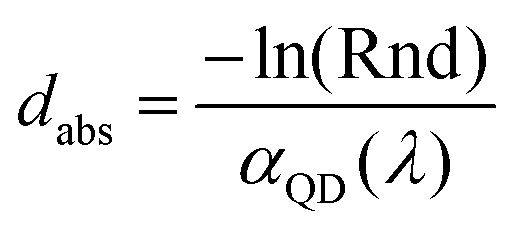 , where αQD(λ) is the attenuation coefficient of the given concentration of luminophores at the wavelength of the ray packet and Rnd is a random number between 0 and 1. If a ray packet reaches an interface, its transmission/reflection is computed (or defined by user input if the interface is with a solar cell) and the reflected portion continues to be traced. If the ray packet is absorbed and re-emitted, the wavelength is randomly selected based on the emission spectrum of the chosen luminophore, with the ray packet intensity reduced according the luminophores PLQY, and a random emission direction is selected. Then the emitted ray packet continues to be traced. Each simulation is based on 106 ray-packets with initial wavelengths chosen to represent the air-mass 1.5 global (AM1.5G) solar spectrum, which was sufficient for the output efficiency to be precise to 0.1% absolute. A screenshot of the main user-page of Raylene v5.21 is given in Fig. S1 of the ESI.†
The input parameters required for ray-tracing of the LSC can be divided into the LSC dimensions, LSC host material, the luminescent material, and solar cell data. These variables are summarised in Table 1 and will be covered in detail below. As previously discussed, many lab-scale LSCs are about 5 cm × 5 cm, which is why 25 cm2 is chosen as a default area. To demonstrate the effects of scaling, square LSCs with areas ranging from 1 cm2 to 100000 cm2 are investigated, with the largest size being similar in area to sheets of architectural glass. The LSC thickness is fixed at 0.3 cm as c-Si solar cells with this active width have been successfully used to fabricate large-area LSCs before.45 This work does not consider the mechanical stability of the resulting LSC modules, the requirements for which are discussed for building envelope materials in the recent work by Huang et al.52
| Parameter | Value | Units | |
|---|---|---|---|
| a Embodies absorption and scattering, both assumed to be wavelength independent. b Defined here as the optical density of a single-pass through the 0.3 cm-thick LSC measured in the short-wavelength region. c As defined in eqn (2), using the PL spectrum as would be measured in a cuvette containing a dilute solution of QDs. d Defined here as the optical density of a single-pass through the 0.3 cm-thick LSC measured in the long-wavelength region. | |||
| LSC waveguide: | |||
| Area | 25 | (1, 10, 25, 100, 500, 1000, 5000, 10000, 50000, 100000) |
cm2 |
| Total host attenuationa | 0 | (0, 10−4, 10−3, 10−2, 10−1, 10−0) | cm−1 |
| QD: | |||
| Absorbance ODb | 1.3 | (0.1, 0.2, 0.4, 0.5, 0.6, 0.8, 1.0, 1.2, 1.3, 1.4, 1.5, 2.0, 2.5, 3.0) | — |
| Absorption | 95 | (21, 37, 50, 60, 68, 75, 84, 87, 90, 94, 95, 96, 97, 99, 99.7, 99.9) | % |
| Emission peak | 1000 | (750, 800, 850, 900, 950, 1000, 1050 1100) | nm |
| PLQY | 100 | (50, 60, 70, 80, 90, 95, 100) | % |
| Overlap integralc | 0.074 | (0.135, 0.074, 0.055, 0.041, 0.019, 0.005, 0.001, 0.00003, 0) | — |
| Absorption tails ODd | 0 | (0.005, 0.01, 0.02, 0.03, 0.04, 0.05) | — |
For the host material, fused silica (SiO2) is employed due to it being a near lossless optical material. For simulation of this material, the dispersive refractive index relation is taken from Palik.53 The refractive index is also similar to other glasses and host polymeric materials used for LSCs,54 thus making a good choice for the simulations. The attenuation coefficient, α, includes contributes from both host absorption as well as scattering. By default, it is assumed that α = 0 cm−1, except in simulations where the effect of the host attenuation coefficient is investigated, in which case values are varied from α = 1 × 10⁻⁴–1 × 10−0 cm−1. It should be noted that the chosen level of host absorption was equal at all wavelengths, which is unlikely to occur in practice. The range for α was chosen based on observations from the literature for common LSC hosts such as: polymethylmethacrylate (PMMA), which exhibits a very wide range of attenuation coefficients (α = 10−4–10−1 cm−1 depending on the preparation technique37,54); fluorinated polyurethane (α ∼ 10−3 cm−150); N-BK7 glass (α ∼ 10−3 cm−1 37); low-iron soda lime glass used in the PV industry (α ∼ 1 × 10⁻¹ cm−1), a high-quality borosilicate float glass (α ∼ 10−2 cm−1); and nearly-lossless fused silica. The decision to use a wavelength-independent value for α is justified as the within the band of all possible peak emission wavelengths (750–1150 nm) the observed variation in α is not great.37 As previously mentioned, the effects of surface scattering are detrimental to waveguiding, but are not explicitly considered here. This can be justified given that surface roughness values for likely large-area substrates – such as borosilicate float glass – have been determined to be <1 nm.55 Furthermore, the scattering loss at the surface could also be considered as bundled into the bulk host attenuation coefficient as the number of surface interactions in the thin slab is high in the large-area devices.
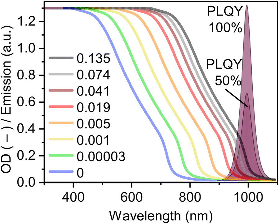
A wide range of luminescent materials have been employed to fabricate LSCs, including fluorescent organic dyes,45,46,56 rare-earth and transition-metal ions,9,57 rare-earth complexes,58,59 antenna-like complexes such as phycobilisomes,60 as well as semiconducting QDs.41,61–63 QDs are chosen in this work given that they exhibit the greatest promise in terms of broad and strong absorption that is tuneable (either with size or chemical composition) and of similarly tuneable emission occurring with a high PLQY. Such QDs can be made from materials such as: (i) CuInS2, which have been recently used to fabricate LSCs with an optical power efficiency of 6.8% over a 30 cm × 30 cm area;41 or (ii) metal halide perovskite QDs.63,64 In this work, methylammonium lead iodide (MAPbI3) perovskite QDs in solution (30 mg mL−1 in hexane) were measured in a 1 cm cuvette to exhibit 100% PLQY at 750 nm and strong absorption in the shorter-wavelength region. This short-wavelength absorbance was implemented in the ray-tracing software as the default optical density of OD = 1, resulting in 90% light absorption during a single pass through the 0.3 cm-thick LSC. A wide range of OD values (0.1–3.0) were investigated to determine the optimum performance for an opaque LSC, but also the region where acceptable performance lies for a semi-transparent LSC. While the absorption and emission spectra for the 750 nm-emitting QDs used in this work were based on experimental results, all longer-wavelength emitting QDs were simply realised via red-shifting the experimentally-realised absorption and emission data. When shifting the absorption spectra to longer wavelengths, the last value was simply used to replace all missing data, which is how the flat absorption spectra (seen in Fig. 2) results. Such a flat absorption spectrum is not likely to occur in practice, unless some of approaches as discussed via Makarov et al.65 are pursued to achieve a more neutral colour balance, noting that this may come at the expense of efficiency. Here, the authors wish to point out that, in reality, one cannot simply vary the absorption and emission spectrum or the PLQY as these are fundamental principles anchored in quantum mechanics. However, for the sake of the present exercise, these are all treated is independent variables in order to identity where the bottlenecks in the LSC energy conversion process lie. Fig. 2 plots the front surface reflectance of the c-Si solar cell along with the IQE (data taken from66), with the latter ideally matching the emission peak of the QDs.
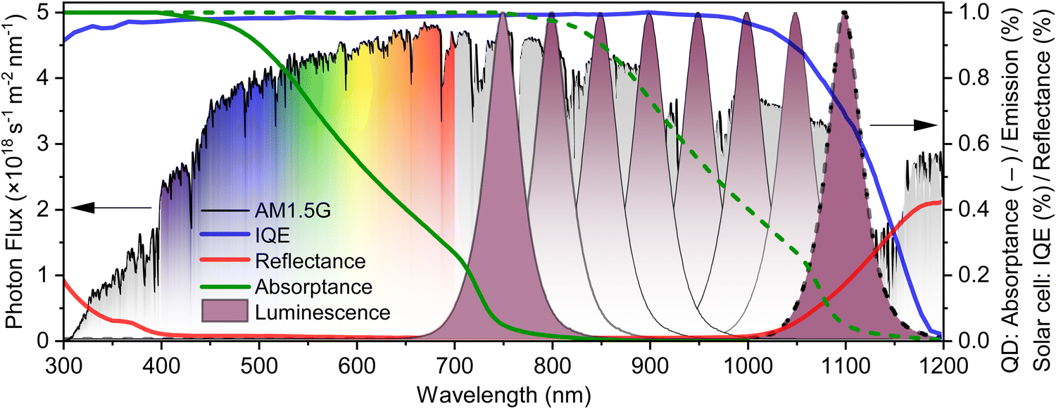 | ||
| Fig. 2 Typical optical input parameters for a ray-tracing simulation of a LSC coupled to c-Si PV, including: (i) the photon flux in the air-mass 1.5 global (AM1.5G) solar spectrum; (ii) the internal quantum efficiency (IQE) and the (iii) reflectance losses of the c-Si solar cells (data taken from ref. 66,67); (iv) the absorptance spectra of a semiconductor quantum dot (QD) with emission peaks at 750 nm (solid lines) and 1100 nm (dashed lines); and (v) how varying this absorptance peak in 50 nm steps matches with the incident sunlight and properties of the c-Si solar cell. Naturally, the absorptance spectra for the QDs emitting at 800–1050 nm also shifts, but these are not drawn for the sake of clarity. | ||
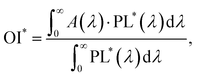
The key weakness of QDs is that they typically exhibit a relatively large spectral overlap (in other words, a small Stokes shift), indicating that multiple re-absorption/re-emission events can be expected to take place over the long optical pathlengths that occur within a LSC. The authors also note this is consistent with the modified overlap integral (OI*) as proposed by Lunt and co-workers,68 which is defined as:
 | (2) |
 , where nh is the index host. For nh = 1.46 there is a 27% chance that the ray-packet from an emission event will be lost in the escape cones. For multiple emission events, the probability for escape cone loss increases as
  , where m is the number of absorption events the ray packet undergoes. For, 2, 3, and 4 absorption events the probability of loss of the packet in an escape cone increase to 47, 61, and 72% respectively. This is consistent with the observed escape cone losses as high as 50–70% of the emitted photons for a luminophore with a significant spectral overlap.71 Therefore, even with a 100% PLQY it is critical to keep the number of absorption events low by minimising overlap integral such that the emitted photons can reach the edges of large LSCs.
As a side note, the decrease in energy of ray packets due to the Stokes shift of the luminophore is irrelevant, since thermalisation losses will occur anyway once the luminescence reaches the edge-mounted solar cell. In theory, the reduce in thermalisation losses in the solar cells could lead them to operate at a slightly lower temperature than a solar cell with the same input photon flux distributed over the solar spectrum, however in a luminescent down-shifting configuration this effect was demonstrated to be minimal.33
An additional problem with some luminescent materials, including QDs, is the presence of absorption tails that often extend well-beyond the emission band. The origins of such absorption tails can be from the polydispersity as well as aggregation during the ligand-exchange process in the synthesis leading to some bulk-like material,72 or trap/charge-induced absorption in some quantum dots. It should be noted that, the effect of the absorption tails is considered in the best-case scenario when this tail reabsorption can still lead to reemission.
The solar cells chosen for application to the edges of the LSC are the fabricated from c-Si, which is the market dominant PV technology, currently comprising about 95% of the world PV market.73 These higher efficiency devices cost around 0.14 € per W.73,74 Furthermore, other works have demonstrated the use of long, thin (10 cm × 0.3 cm) strips of c-Si solar cells to fabricate large-area LSCs.45 The highest efficiency c-Si solar cells existing today are: (i) based on a heterojunction, formed between an intrinsic c-Si wafer sandwiched between ultra-thin amorphous silicon layers; and (ii) possess interdigitated back contacts, whereby all the metal electrodes are on the rear of the device, thus exhibiting extremely low front surface reflectance losses. The solar cells used in the ray-tracing simulations exhibit an efficiency of 26.7%, an open-circuit voltage (VOC) of 738 mV, a short-circuit current density of 42.6 mA cm−2, and a fill-factor of 84.9%, while the IQE and reflectance spectra are given in Fig. 2 (using data from ref. 66 and 67).
In each of the sections below, ray-tracing simulations were employed to investigate a wide range of parameters and values and understand the factors limiting LSC technology.
3. Figures-of-merit of LSC performance
Firstly, to get an overview of the insights that can be obtained from Raylene, a 10 cm × 10 cm LSC exhibiting a total host attenuation of α = 10−2 cm−1 containing QDs (concentration OD = 1.0, emitting at 900 nm with a PLQY of 80%, OI* = 0.135) was investigated. The fate of 106 rays originating from a normally incident AM1.5G solar spectrum (300–1400 nm range) are traced and plotted in Fig. 3. The Sankey diagram in Fig. 3A (integrated over all incident wavelengths) indicates that 3.4% of rays are lost due to front-surface reflectance, which is difficult to alter this since this is governed by Fresnel's equation. It is noted that adding an anti-reflection coating (ARC) does not provide any benefit here since such losses are difficult to address due to Helmholtz reciprocity, i.e. if an incident light ray experiences improved optical in-coupling, then a greater fraction of the emitted luminescence will also be out-coupled. (There is an exception, which will be discussed in Section 6.4). Of the rays that enter the LSC, a large number (58.1%), mostly at longer wavelengths where the luminophore no longer absorbs, are transmitted through the LSC. The remaining fraction (38.5%) encounter a QD and are absorbed, and could contribute to the short circuit current (ISC) generation in the solar cells. However, this is decreased by 16.2% as this is the percentage of total incoming AM1.5G photons that are lost due to non-radiative recombination resulting from sub-unity PLQY (80% in this example). Furthermore, a total of 14.4% of the total incoming rays are lost due to emission that escapes from the front or back surface (like the non-radiative recombination this can occur on the first or a subsequent absorption event). Finally, 0.8% of the initial rays are absorbed by the host. This leaves 3.0% of the total incoming AM1.5G spectrum of rays that contribute to a the ISC of the LSC module. A graphical representation of the fate of the 1 million incident photons as a function of the incident wavelength is presented in Fig. 3B.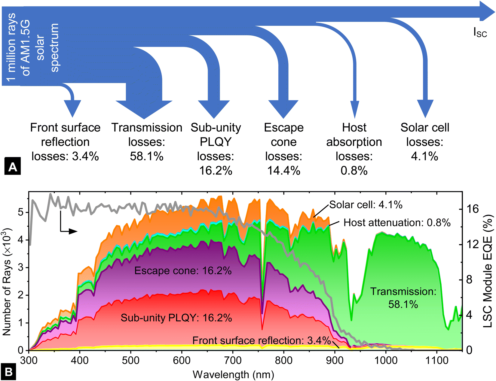 | ||
| Fig. 3 Performance summary of a 10 cm × 10 cm × 0.3 cm LSC exhibiting a total host attenuation of α = 10−2 cm−1 containing QDs (concentration OD = 1.0, emitting at 900 nm with a PLQY of 80%, and a modified overlap integral of OI* = 0.135) and with c-Si solar cells attached to all four edges. (A) Sankey diagram illustrating the fate of the 106 rays incident from the AM1.5G solar spectrum and the fraction that end up contributing to the short-circuit current (ISC) of the LSC module. (B) The same fraction of rays as depicted above, but now as a function of wavelength, along with the external quantum efficiency (EQE) of the LSC module. | ||
From the ISC found through the above number of rays that are absorbed by the solar cells, the power produced by the solar cells can be estimated by multiplying the predicted ISC by the VOC and fill factor. This means that the following figures-of merit can be defined from the simulations.
• LSC power conversion efficiency (ηLSC) defined as the electrical power collected from edge-attached solar cells divided by the optical power impinging on the face of the LSC. This is the key figure-of-merit and allows direct comparison with other solar energy conversion technologies. In the above example (Fig. 3), the ηLSC would be 5.1%. In practice, the ηLSC can be measured by taking the current–voltage (I–V) curve of the solar-cells attached to the LSC when illuminated under standard test conditions (STC – defined as 1000 W m−2 of AM1.5G solar spectrum and with the device held at 25 °C). Note, at this stage no assumptions are made as to how the solar cells are interconnected, but it is important that all four edges are fully covered. If all edges are not covered then the remaining edges should be blackened and roughened to prevent any over-estimate of ηLSC (see Yang et al.75 for more details).
• Escape cone losses (ECL): defined as the number of emitted photons from that depart out of the front or rear faces of the LSC. As mentioned above, this represents a major losses mechanism for the LSC technology, but remains difficult to address.
• LSC waveguiding efficiency (ηwave) defined as the percentage of incoming photons (from an AM1.5G distribution) that are absorbed by the edge-mounted solar cells. In the above example this is 3%. Note that this definition is similar to the overall optical efficiency used by some researchers.76
• Concentration ratio (C): defined here as the ratio of the electrical output power of the LSC to the power that would be generated by taking same strips of c-Si solar cells (with an area APV, that is smaller than ALSC) along the perimeter and then facing these directly towards the sun (under STC). In other words, this indicates how much higher the photocurrent in the solar cells are compared to if they were just rotated to face the same direction as the LSC. For the LSC described above, C = 4.2×. Note, in many small area LSCs, the concentration ratio is sub-unity,24 in which case these devices are actually de-concentrators.
• Average visible transparency (AVT): is important for any semi-transparent PV technology and is defined as the fraction of light that the human eye can detect that is transmitted through the LSC, calculated using:77
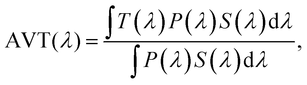 | (3) |
• Colour: To evaluate the colour fidelity, the colour rendering index (CRI) was determined using the standard CRI L*a*b* space model (as recommended by Lunt and co-workers75,78), where the parameters are defined as: L* is the luminosity of the colour, while a* is the red or green component of the colour, and b* is the yellow or blue component. For completeness, this is also reported in terms of RGB colour coordinates. The colour purity is used to quantify the degree of saturation on the CIE 1931 chromaticity diagram.
The following section considers how a variation in these input parameters affects the LC performance, with focus on revealing how a reasonable efficiency can be maintained at large area.
4. Optimisation for lab-scale (25 cm2) LSCs
4.1 Emission wavelength and optical density
Regardless of whether an opaque or semi-transparent LSC is being engineered, the first step towards achieving high efficiency is via choosing the right properties of the QD, such that (i) a suitable broad range of sunlight can be absorbed; (ii) the emission matches well to the solar cell EQE; and (iii) the doping concentration of the QDs in the LSC is optimised. Thus, the first parameters to be varied were the peak emission wavelength of the QDs – ranging from 750 to 1100 nm (as illustrated in Fig. 2) – along with their optical absorption (OD), defined as the fraction of short-wavelength absorbed in a single-pass through the LSC. A wide range of ODs for the QDs were investigated – as high as OD = 3.0 (99.9% absorption) down to OD = 0.1 (21% absorption) as well as many other values in-between (2.5, 2.0, 1.5, 1.4, 1.3, 1.2 1.0, 0.8, 0.6, 0.4 and 0.2). This range was chosen to cover all possibilities for very opaque higher-efficiency LSCs to lower-efficiency semi-transparent replacements for windows. Naturally, as the OD changes, so to does the chance for reabsorption as the emitted photons travel in the waveguide.The results are displayed in the contour plot of Fig. 4, which maps the peak emission wavelength and the OD against the LSC electrical efficiency. It can be seen that the best performing LSCs are comprised of QDs with a peak emission wavelength around 1000 nm range and with an OD of 1.0 to 1.5. Within this relatively broad regime it is possible to fabricate an opaque LSC with an efficiency of >10%. At lower ODs, the performance is worse due to the reduced fraction of solar photons absorbed and the device starts to become semi-transparent. At OD > 1.5, the ηLSC reduces as the probably for self-absorption also increases, which will be discussed in detail in the next section. While the 1100 nm-emitting QD is certainly expected to absorb more photons in the red/NIR region of the solar spectrum, it should also be noted that the solar cell IQE starts decreasing beyond 1000 nm. In addition, the reflectance losses of the solar cells in this wavelength range are also increasing significantly. Both of these factors contribute towards a relatively rapid reduction in ηLSC beyond 1050 nm. At shorter emitting wavelengths, there is a gradual reduction in performance simply due to a smaller fraction of sunlight being absorbed. Thus, 1000 nm-emitting QDs are used throughout the remainder of this work.
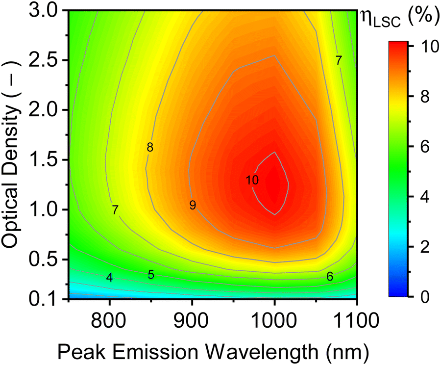 | ||
| Fig. 4 Contour plot demonstrating the achievable energy conversion efficiency of a LSC (5 cm × 5 cm × 0.3 cm, SiO2 waveguide, PLQY = 100%) as a function of the QD optical density and peak emission wavelength. For maximum performance, QDs with a peak emission wavelength of ∼1000 nm should be used and an opaque LSC can exhibit ηLSC ≥ 10% when using an OD of 1.0–1.5. (Simulation parameters: OI* = 0.074, zero host attenuation, c-Si solar cells attached to all four sides, 1 million rays). | ||
A recent paper by Huang et al. recommended that semi-transparent PV technologies should have an AVT of ≥50% to balance optical power contributions to both daylighting and electricity generation.52,76 For a 1000 nm peak emission wavelength the AVT, OD, and in ηLSC are summarized in Table 2. It can be seen that a 47% AVT is achieved using OD = 0.3 and at this value a ηLSC of 6.3% can still be achieved for a 25 cm2 LSC. Unsurprisingly, moving towards a lower OD increases the possible AVT, and vice versa. Also shown in Table 2 is the indicative colour of such LSCs, the grey tone resulting from the neutral colour balance, with the 1000 nm-emitting QDs absorbing all visible wavelengths equally (noting that this would not be the case if, for example, a 750 nm peak emission QD was chosen). For completeness, the fraction of light transmitted (λ = 380–780 nm) of each of the five semi-transparent LSCs are plotted in Fig. S2 (ESI†), along with colour fidelity (CRI L*a*b*) and colour purity (CIE1931).
| OD (−) | AVT (%) | η LSC (%) | Colour (CIE1931 & RGB coordinates) |
|---|---|---|---|
| 0.1 | 76 | 2.7 | CIE1931 (0.313, 0.329) RGB (225, 226, 224) |
| 0.2 | 60 | 4.8 | CIE1931 (0.313, 0.329) RGB (203, 204, 202) |
| 0.3 | 47 | 6.3 | CIE1931 (0.313, 0.329) RGB (183, 183, 181) |
| 0.4 | 38 | 7.5 | CIE1931 (0.313, 0.329) RGB (166, 165, 163) |
| 0.5 | 30 | 8.3 | CIE1931 (0.313, 0.329) RGB (148, 149, 147) |
4.2 PLQY and Overlap Integral
 | ||
| Fig. 5 Graphical representation of the overlap integral range (OI* = 0–0.135) of the QDs chosen for an opaque LSC (QD concentration equivalent to OD 1.3) with a peak wavelength emission at 1000 nm at either a unity or sub-unity (50%) PLQY. | ||
The key result of how the LSC energy conversion efficiency tracks both of these parameters is plotted in Fig. 6A. It can be seen that reducing the OI* to 0.019 and a using a PLQY of 100% results in the maximum ηLSC approaching 12% being reached. This is due to a greatly decreased maximum number of re-absorption/re-emission events within the LSC. Fewer re-absorption events will results in significantly reduced ECL, which are plotted in Fig. 6B. At 100% PLQY, the ECL is observed to decrease from 57% at high OI* down to 26% at low OI* values, which is the value expected for a LSC fabricated from a n ∼ 1.5 waveguide.8 However, ηLSC decreases as the degree of OI* is further reduced (Fig. 6A), which is due to the fewer AM1.5G photons being absorbed. The low ECL values (10–20%) for OI* ≥ 1 occur at low PLQY values (50–60%) as then the re-absorbed photons have a lower chance of being re-emitted. The waveguiding efficiency shown in Fig. 6C follows a similar trend to Fig. 6A, with the highest ηwave values of 74% occurring at the highest PLQY and lowest OI*. It is also pointed out that in such a case, with no other optical losses present, ηwave = 100% – ECL. At the other end of the spectrum (low PLQY and high OI*), very low ηwave values of down to 10% are reported, even in the present small-area LSC. Whether the resulting LSC will exhibit a concentration ratio of C > 1 or not (i.e. acts as a concentrator) hangs in the balance of the OI* and PLQY parameters, with the possible range being from C = 0.3–1.7 (Fig. 6D).
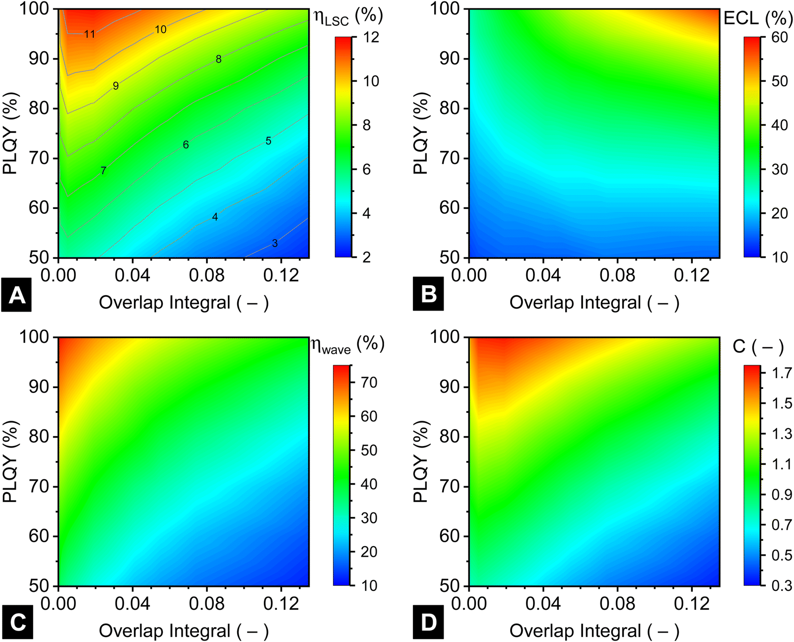 | ||
| Fig. 6 Performance of opaque (OD = 1.3) based on QDs emitting at a peak wavelength of 1000 nm as a function of overlap integral (OI* = 0–0.135) and PLQY (50–100%): (A) electrical conversion efficiency (ηLSC); (B) escape cone losses (ECL); (C) waveguiding efficiency (ηwave); (D) concentration ratio (C). (simulation parameters: LSC dimensions 5 cm × 5 cm × 0.3 cm, zero host absorption losses, c-Si solar cells attached to all four sides, 1 million rays). | ||
Thus, while a small OI* (or, conversely, a large Stokes shift) has often been recommended in the LSC literature,29,37 it is important to note that, in the case that the steepness of the absorption and emission curves are fixed (and assuming that these are realistic and therefore not infinitely steep), there is an optimum. In this case, the absorption and emission must be shifted apart to reduce the overlap, and low OI* values start to reduce the absorption of sunlight (causing the LSC performance to decrease correspondingly). Also, maintaining a high PLQY is important, since, for example, when using QDs with a 90% PLQY instead of 100%, the maximum ηLSC already drops to 11.6% (1.5% absolute lower than the best performing LSC at 100% PLQY).
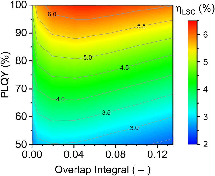 | ||
| Fig. 7 η LSC as a function of PLQY and OI* for a semi-transparent LSC based on 1000 nm peak emitting QDs, where the OD for each scenario was adjusted such that each exhibited an AVT of 50%. (Simulation parameters: LSC dimensions 5 cm × 5 cm × 0.3 cm, zero host absorption losses, c-Si solar cells attached to all four sides, 1 million rays.) | ||
5. Optimisation for pilot- and commercial-scale LSCs
5.1 Scale-up of small-area LSC solution
The best performing opaque LSC from the previous section (OD = 1.3, 1000 nm emission, OI* = 0.019, 100% PLQY) was selected for further scale-up investigations. The first goal was to understand the impact of host attenuation coefficient (from 10−4–100 cm−1) as the LSC area increased from 1 cm2 to 100000 cm2 (3.16 × 3.16 m or 10 m2), with the results plotted in Fig. 8. From Fig. 8A, it can be seen that with a well-chosen luminescent material, LSC energy conversion efficiencies >13% for a wide range of host attenuation values (roughly 10−4–10−1 cm−1) as long as the LSC area is very small (<5 cm2). However, as the LSC area increases, the ηLSC is observed to steadily decrease as optical pathlengths increase, again due to an increasing number of re-absorption/re-emission events. This, in turn, dramatically increases the chance that luminescence leaves the LSC, with ECL now reaching values of up to 94% for the largest LSCs (Fig. 8B). Secondly, as host attenuation increases, the decrease in ηLSC occurs much earlier. Thus, Fig. 8A indicates that with the chosen QDs it is only going to be possible to fabricate a LSC of 25 cm2 with an energy conversion efficiency of nearly 12% at best, while for larger LSCs of 1000 cm2 (31.6 cm side lengths) and 100000 cm2 (3.16 m side lengths) a maximum ηLSC of about 6.5% and 1%, respectively, can be achieved. A further take-away message from Fig. 8A is that LSCs are largely tolerant of host attenuation in the range 10−4 cm−1 to 10−2 cm−1, with only small performance reductions being observed. In other words, the reabsorption-driven ECLs are playing a much greater role here, which points towards the importance of developing luminescent materials that exhibit zero-reabsorption. The same messages are echoed in the ηwave results plotted Fig. 8C, whereby: (i) for small LSC areas, performance is nearly independent of the host attenuation coefficient; however (ii) for larger areas (anything >10 cm2) the fraction of waveguided emitted photons starts dropping steadily reaching <5% for commercial-scale (100000 cm2). Fig. 8D illustrates that a large-area LSCs based on the present QDs could achieve up to 9× concentration – if the host attenuation remained less than 10−3 cm−1 – but remembering that the energy conversion efficiency of such a device will still be only ηLSC ∼ 1%.
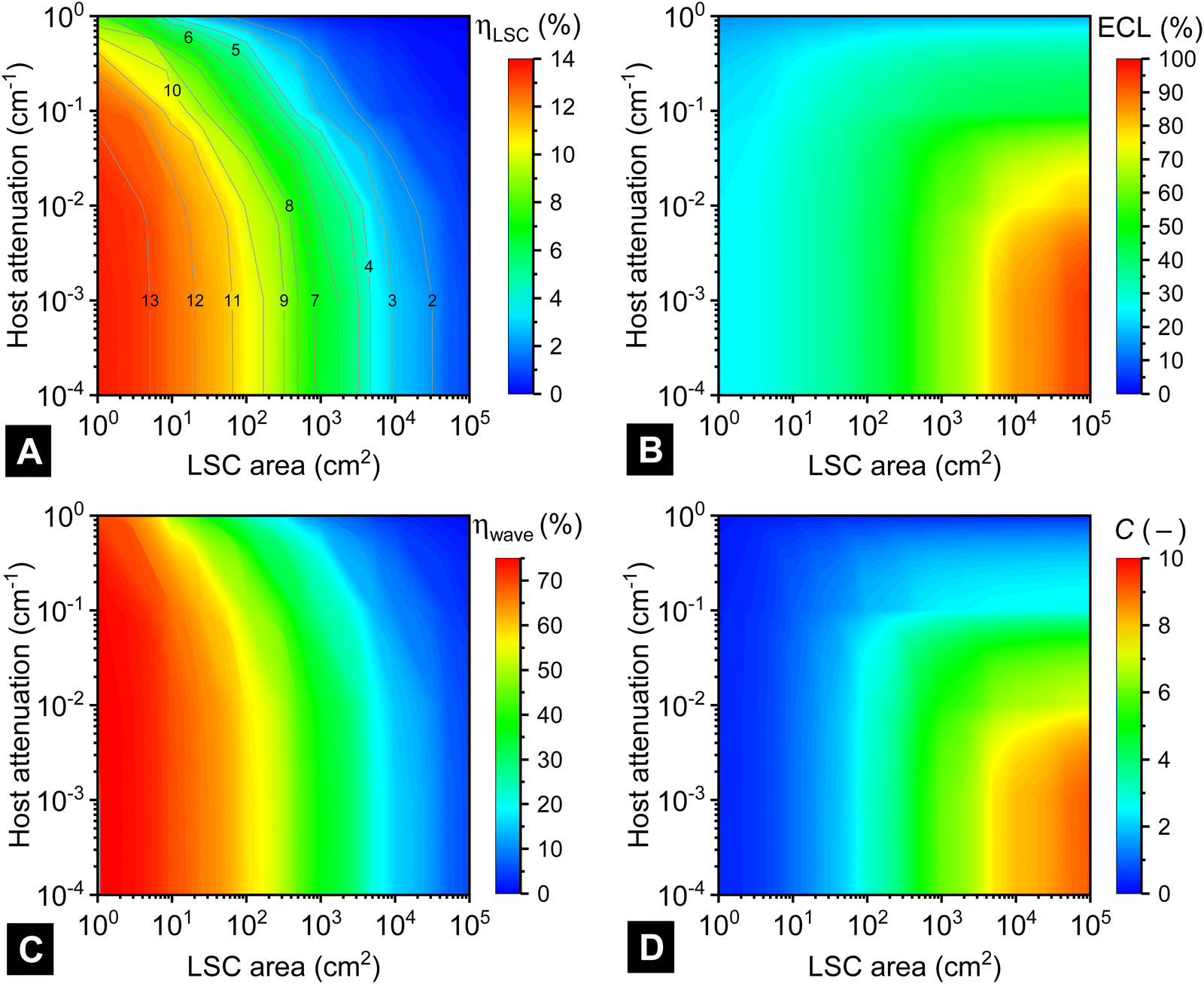 | ||
| Fig. 8 Contour plots indicating the effects of increasing the area (1–100000 cm2) and host absorption (from 10−4–100 cm−1) of an opaque LSC on (A) ηLSC; (B) ECL; (C) ηwave; (D) concentration ratio C. (Simulation parameters: 0.3 cm thickness, 1000 nm peak emission, OD = 1.3, 100% PLQY, OI* = 0.019, c-Si solar cells attached to all four side, 1 million rays.) | ||
5.2 Re-optimised QD properties for large-area LSC solutions
To evaluate whether the trends observed in Fig. 6 for the lab-scale devices still hold true for a pilot- and commercial-scale LSCs, the same analysis of varying the OI* and PLQY is performed again, but this time for a 1000 cm2 and 100000 cm2 LSC in both semi-transparent (AVT = 50%) and opaque (OD = 1.3) architectures.
The results for the opaque pilot-scale LSCs (1000 cm2 area) are displayed in Fig. 9A. The most noticeable trend is that the ηLSC value drops off dramatically with OI* values >0.008, while a linear reduction in ηLSC is observed with decreasing PLQY. Thus, while a ηLSC > 9% can be achieved with OI* < 0.008 and PLQY > 90%, even if the same PLQY is maintained the ηLSC drops to ∼5% at OI* ∼ 0.03 and drops even further at higher OI* values. The situation becomes somewhat more relaxed for the semi-transparent pilot-scale LSC (Fig. 9B) where the maximum ηLSC value (∼5%) can be achieved now for an OI* value of about 0.006. The drop-off towards higher OI* values is noticeably less steep in Fig. 9B than in Fig. 9A.
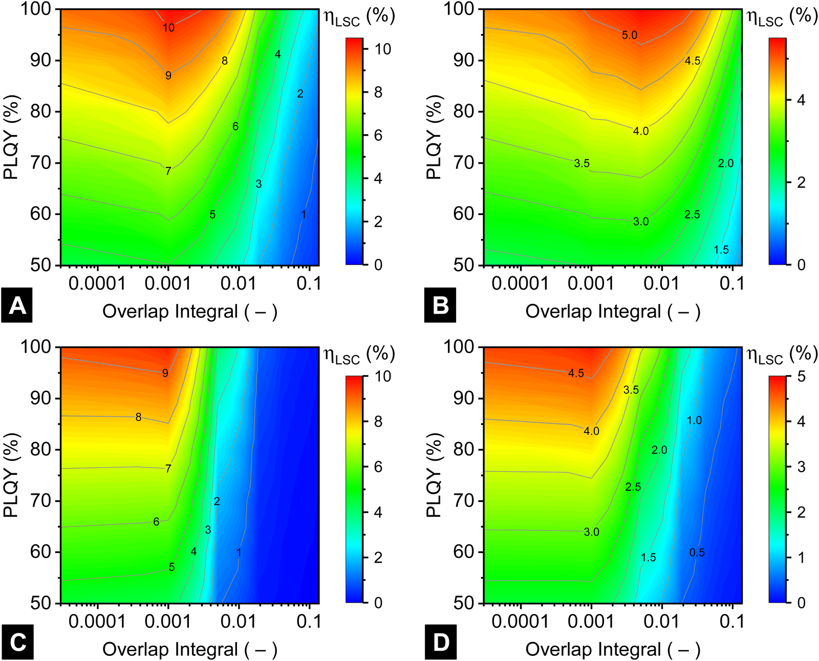 | ||
| Fig. 9 Revisiting the effects of the overlap integral (OI* = 0.00001–0.135, noting the logarithmic scale on the x-axis) and PLQY (50–100%) and a peak wavelength emission of 1000 nm (as investigated earlier in Fig. 5A), but this time for: (A and B) 1000 cm2 (pilot-scale) LSC that is either (A) opaque (OD = 1.3) or (B) semi-transparent (OD = 0.3–0.44); (C and D) 100000 cm2 (commercial-scale) LSC that is either (C) opaque (OD = 1.3) or (D) semi-transparent (OD = 0.3–0.44). (Simulation parameters: zero host absorption losses, c-Si solar cells attached to all four sides, 1 million rays.) | ||
The result for 100000 cm2-area opaque LSCs (see Fig. 9C) demonstrates that indeed a high energy conversion efficiency of >9% is achievable in the best case. To achieve this though, it is imperative that the PLQY remains very high (>95%) and that the OI* remains very low (<0.001). As discussed above, the OI* is the critical parameter here, and as soon as its value exceeds 0.005, it becomes impossible to fabricate an LSC module with an efficiency of even ηLSC = 3%. For the semi-transparent 100000 cm2-area LSC (Fig. 9D), again the situation is similar to the opaque case with an OI* < 0.002 being required to achieve the maximum ηLSC values of >4.5%. While the drop-off with increasing OI* is not as steep, the OI* threshold of about 0.001 remains the make-or-break point.
While such energy conversion efficiencies might sound small, if these could be truly realised on the 10 m2-scale for BIPV then it would be a real breakthrough. This is almost twice the size of the largest-ever fabricated PV modules, a 5.72 m2 thin-film PV module developed by Applied Materials.79 Such thin film modules – based on tandem stack of amorphous silicon on microcrystalline silicon, both hydrogenated – reached stabilised efficiencies of just over 10% on smaller area (1.43 m2) modules and preliminary results suggested that such efficiencies could be translated across to the larger format modules, however by 2010 the global economic crises and an over-supply of c-Si saw the investment in such technologies die off. Today, Sunovation in Germany5 are able to manufacture coloured, patterned and even curved BIPV modules based on c-Si solar cells with areas up to 8 m2. Any architect considering installing a semi-transparent LSC as a BIPV technology is will be faced with the option of generating of 450 W from a 10 m2 area waveguide/window (ηLSC = 4.5%) or considering existing off-the-shelf PV technologies. For example, the same amount of power could be generated from an area of just over 2.2 m2 using highly-efficient commercially-available c-Si PV modules with η = 22.6%, leaving 7.8 m2 of free-area to be used for standard architectural double- or triple-glazing.
The trend in the results, looking from Fig. 6A to 9, demonstrates that for the LSC technology to have a hope of transitioning from lab-scale to commercial-scale it is of utmost important that early-stage R&D targets the development of QDs that exhibit: (i) an extremely small OI* (ideally < 0.001); and (ii) a very high PLQY (ideally > 95%). The results from Fig. 9 also indicate that 1000 cm2 is an excellent size for a pilot-scale device, since if the device works well on that scale then the majority of the big problems have already been solved and further scale-up efforts are warranted.
In summary, high ηLSC values of 10% and 5% can be achieved on pilot-scale LSCs in opaque and semi-transparent architectures, while on the commercial-scale devices this value reduces slightly to 9% and 4.5%. To achieve any of these target values though, it is imperative that the OI* remains very low (<0.001) and that the PLQY remains very high (>95%), otherwise re-absorption processes (followed by ECL) will quickly reduce the conversion efficiency to a very low level.
6. Re-absorption losses: further analysis and potential solutions
6.1 Absorption tails
The negative impact of absorption tails on LSC performance has been examined in detail experimentally for fluorescent organic dyes.80,81 For example, Wilson et al. demonstrated that for a Lumogen F Red 305 doped LSC of dimensions 60 × 60 × 0.3 cm, the absorption tail of the dye extends out to 750 nm exhibiting a value of about 3.5 × 10⁻³ cm−1.81 Thus, the absorption tail extends across the entire emission spectrum of the dye. Earp et al. investigated commercially-fabricated LSC strips of up 1.2 m in length doped with Lumogen F Yellow 083 dye, determining that there was nearly 16% absorption in the tails region (550–750 nm, beyond the main absorption band centred at around 500 nm.80 After 6 days of outdoor exposure (under a UV blocking cover that prevented λ < 340 nm light from reaching the LSC), the tail absorption fraction increased to nearly 35%, with as similar effect being observed for other perylene-based dyes as well.80 The authors suggested that these absorption tails are due to interactions of the dye with impurities in the PMMA matrix, resulting in a photooxidation reaction, or residuals of the MMA monomer (present at <0.3 wt%).80The effect of absorption tails can also be very pronounced in perovskite materials. For example, in recent works determining the optical constants of CsPbBr3 and CsPbI3 thin films via spectroscopic ellipsometry, a non-negligible extinction coefficient can be observed extending well beyond the emission bands.82,83 This effect is also observed in perovskite QDs, even before effects of the polymer matrix are considered.84 Here, the effect of absorption tails are examined via increasing the long-wavelength OD of the perovskite QDs by 0.005 to 0.05 (defined at 1100 nm), as illustrated in Fig. 10A. The range for the absorption tails OD was chosen to span mild to severe effects for a variety of LSC areas: lab-scale (25 cm2), pilot-scale (1000 cm2) and commercial-scale (100000 cm2). Two things to note here are that: (i) the OD for all samples was kept constant in the region 300–918 nm; and (ii) the absorption was assumed to be non-parasitic (i.e. re-emission could result), noting that if the tail absorption would be parasitic then it can be regarded in the same manner as host absorption, as already discussed above. One key result is plotted in Fig. 10B for the pilot-scale (1000 cm2) LSCs, with the remainder being presented in Table S1 (ESI†). From Fig. 10B, it can be seen that the impact of the absorption tails on the 1000 cm2 LSC results in a steady loss of the achievable LSC energy conversion efficiency, with ηLSC reducing from 6.6% down to 5.4% at ODtail = +0.005 and by ODtail = +0.05 the value for ηLSC is only 2.2%. This reduction is attributed the escape cone losses increasing from 63% to 88%; or, conversely, ηwave decreasing from 37% to 12%. As might be expected, the increased tail absorption has (see Table S1, ESI†): (i) a more limited impact on the 25 cm2 LSC, decreasing ηLSC from 11.8% to 9.0%; and (ii) a more pronounced effect on the commercial-scale LSC, with the ηLSC dropping from a maximum of 1.0% down to 0.2%. For the latter LSC, the values for ηwave and the concentration ratio C are already 94% and 9.1× without absorption tails, then becoming 99% and 2.1×, respectively, at ODtail = +0.05 (see Table S1, ESI†).
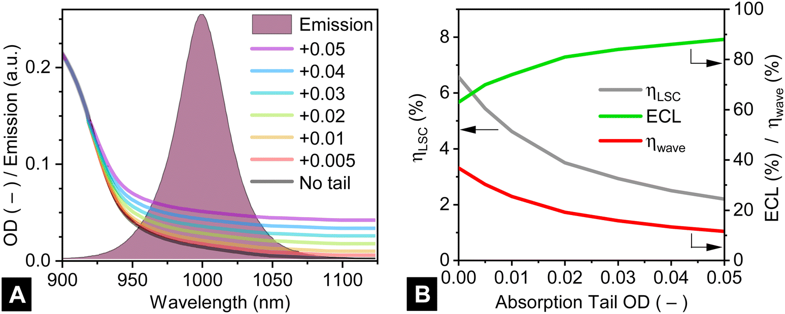 | ||
| Fig. 10 (A) The presence of absorption tails in the luminescence species – simulated here as having an additional 0.01–0.05 OD in the long wavelength region – can have a considerable impact on LSC performance, illustrated in (B) for an opaque 1000 cm2-area LSC in terms of energy conversion efficiency of the LSC, decreasing significantly due to the limited waveguiding efficiency (ηwave) and the high escape cone losses (ECL). The complete results for 25 cm2, 1000 cm2 and 100000 cm2 LSCs are given in Table S1 in the ESI.† (Simulation parameters: 0.3 cm thickness, OD 1.3, 1000 nm peak emission, OI* = 0.074, 100% PLQY, c-Si solar cells attached to all four sides, 1 million rays.) | ||
6.2 LBIC analysis of re-absorption losses
From the above discussion that relates to QD re-absorption and the ensuing ECL, it can be seen that this is the key bottleneck in LSC performance. This is investigated further here via a simulated laser-beam-induced current (LBIC) measurement, which is commonly used to locally characterise PV devices. In the experiment, a simulated laser beam (532 nm, 100 mW cm−2 intensity) is traversed along the top surface of an opaque commercial-scale LSC, from the centre of an edge to the middle of the LSC (as detailed in Fig. S3, ESI†).The results are plotted in Fig. 11, where the 532 nm excitation is traversed away from the edge (starting x = 10−7 cm) – initially in very small steps – towards the centre of the commercial-scale LSC (x = 158.11 cm). It is clearly apparent that the ECL and waveguiding efficiency (ηwave) are inherently related via the simple relationship: ECL = 100% – ηwave. Focusing initially on the high OI* case (OI* = 0.041, solid lines in Fig. 11), at very small distances from the edge, the probability of capturing the resulting QD emission (at least within one hemisphere) is high, with the resulting ECLs remaining relatively low (<40%) and the waveguiding efficiency high (ηwave > 60%). However, already after being 2 cm away from the edge, the ECL have increased to 66%. This trend continues such that at 15 cm from the edge, the ECL is now 90%, while, finally, at the centre of the LSC nearly no luminescence reaches any of the four edges (ECL = 99.7%) and the ηwave < 0.3%. Thus, the zone towards the centre a large LSC becomes increasingly a “dead-zone” and is no longer harvesting any solar energy. In the present case the majority of the collected photocurrent comes from a 10 cm-wide rim around the edge of the LSC and the remaining central area (>87% of the total area) is inactive. Now switching to the low OI* case (OI* = 0.001, dotted lines in Fig. 11), the ECLs rise from 16% at the edge to 35% when excited at the centre, which represents a dramatic improvement over the high OI* case. It should also be noted that the degree of OI* plays a big role in light collection even for luminescence generated right at the edge of the LSC. Correspondingly, the waveguiding efficiency is also improved with ηwave values of 65% being realised at the centre of the LSC, having decreased from 83% when excited very close to the edge.
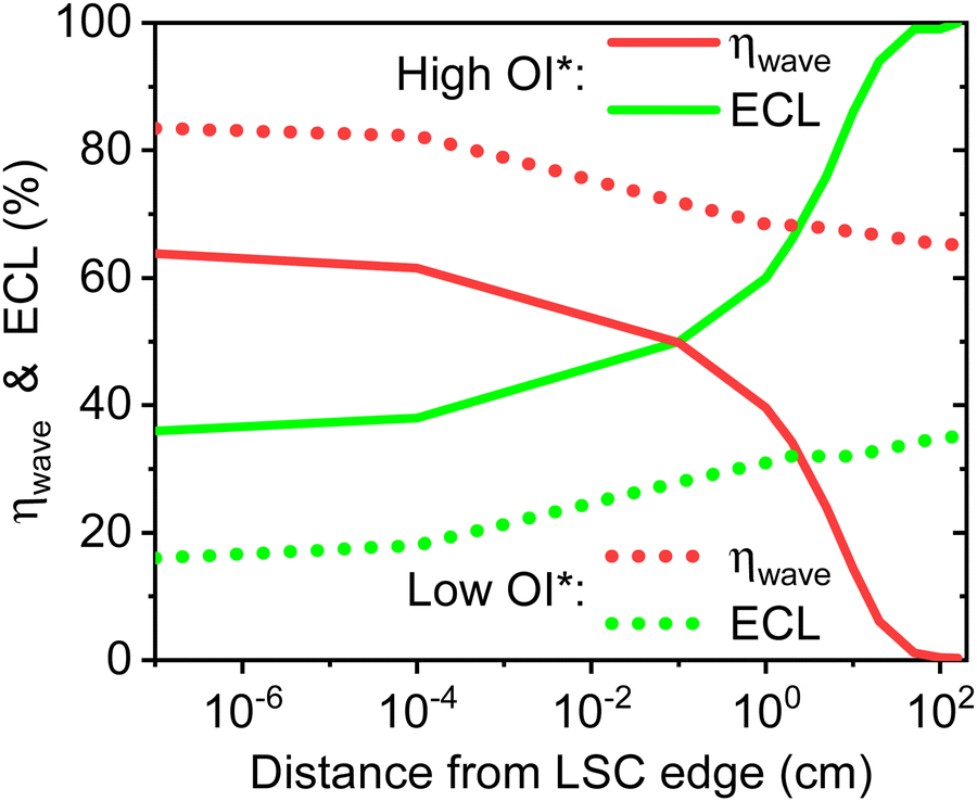 | ||
| Fig. 11 Simulated laser-beam-induced current (LBIC) measurement of two commercial-scale (100000 cm2) opaque LSCs as a 532 nm beam is traversed from the edge of the LSC (x = 10−7 cm) towards the centre (x = 158.11 cm) and its effect on ηwave and ECL: with high OI* = 0.041 (solid lines) and with low OI* = 0.001 (dotted lines). (Simulation parameters: 0.3 cm thickness, OD 1.3, 1000 nm peak emission, 100% PLQY, c-Si solar cells attached to all four sides, 1 million rays.) | ||
6.3 Zero-reabsorption luminescent materials
The key technical solution for the LSC technology is the pursuit of luminescent materials that exhibit zero reabsorption, meaning that the number of absorption/emission events will be limited to unity and the ECL will only be suffered once. A wide range of zero-reabsorption materials have been investigated in the past, ranging from rare-earth complexes58,59 to the work of the van der Kolk group on halide thin films doped with divalent thulium (Tm2+).85 In the area of QDs, research has targeted type-II core-shell QDs, engineered CdSe/CdS nanomaterials with especially thick shells exhibiting low OI*,86–88 as well as Mn2+-doped ZnSe/ZnS QDs.61 Finally, aggregated-induced materials have demonstrated large Stokes shifts, which are realised via a Förster resonance energy transfer (FRET) donor–acceptor pair.89 While many of these materials exhibit significantly reduced self-absorption, it is, in most cases, still non-zero. Thus, a strong recommendation from this work is for material scientists to characterise and quantify the OI* extremely carefully using QD concentrations that are suitable for real-world applications. As emphasised in both Fig. 6A and 9 above, a natural trade-off here is that zero reabsorption is achieved at the expense of collection fewer incident photons. In the case of Fig. 6A (lab-scale LSC), a relatively broad OI* can be tolerated while only suffering a minor penalty on the final LSC efficiency, however this is definitely not the case once large-scale devices (Fig. 9) are to be realised. Thus, when engineering the OI*, a real target would be achieving values of OI* < 0.001.The authors highlight the possibility of separately harvesting the UV and NIR components of the AM1.5G solar spectrum via a tandem LSC, which can circumvent the direct trade-off between AVT and the resulting ηLSC. Yang et al. demonstrated a 5.08 cm × 5.08 cm tandem LSC whereby the UV and NIR harvesting – containing hexanuclear nanoclusters and organic small molecules, respectively – are sandwiched together using a n = 1.30 interlayer, which achieved ηLSC = 3.1% at an AVT of 75.8%.90 However, one cannot escape re-absorption, which now needs to be addressed for both layers, noting that in this example the NIR-emitting BODIPY-dye exhibits a very small Stokes shift (whereas the minimal overlap in the UV harvesting layer is far less problematic).
6.4 Hot-mirrors for reducing ECL
A hot-mirror (HM) is a spectrally-selective dielectric filter that is able to transmit shorter wavelength light, while reflecting longer wavelength light, and are typically employed to protect heat-sensitive elements. HMs can also be combined together with a LSC to mitigate the ECLs, resulting in luminescence that would have departed via the escape cone instead being reflected back to the LSC, as illustrated in Fig. 12A. Originally proposed in 2004, Richards et al. demonstrated that the application of a HM in a Nd3+–Yb3+-doped glass LSC (2.5 × 2.5 cm) resulted in a significant gain in edge-detected luminescence and thus a reduction in ECL.91 Subsequently, Debije et al. investigated the application of a chiral nematic liquid crystal based reflector on 5 cm × 5 cm LSCs and reported a 35% enhancement of light out-coupling at the edge.92 Goldschmidt and co-workers also presented a design for coupling a LSC (2.1 × 2.1 cm) between two spectrally-selective filters and realised a 19% enhancement.56,93 An example of a larger-area LSC implementing a HM can be found in the solar-pumped laser work by Masuda et al.18 In that work, the 30 cm-diameter LSC is based on a liquid medium, meaning that the use of air gaps to realise TIR cannot be realised and thus the only way to prevent light from escaping the system is via the use of a dielectric mirror. In a more recent work, Dottermusch et al. demonstrated that the addition of a HM to a 30 cm-diameter solid-state LSC can enhanced the amount of power absorbed near the edge by up to 50%, depending on the LSC architecture chosen.50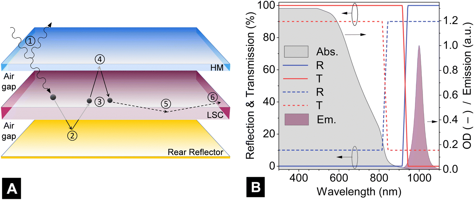 | ||
| Fig. 12 (A) Illustration of the concept of adding a hot-mirror (HM) inf front of a LSC, along with a classical reflector (either specular of diffuse) on the rear side to mitigate the effect of ECL. In addition to the steps described in Fig. 1, here it should be noted that: ① additional reflectance losses will be encountered via the addition of the HM due to the underlying air gap; ② QD luminescence passing out via the rear of the LSC will be returned via the rear reflector; ③ whereupon some of it can be reabsorbed by another QD, re-emitting luminescence isotropically; ④ luminescence in the forward direction that passes within the escape cone can be reflected back to the LSC via the HM; ⑤ thus, increasing the chance of luminescence to be waveguided within LSC via TIR to ⑥ the edges of the LSC. (B) A plot of how the reflection (R) and transmission (T) properties of the hot-mirror change as a function of wavelength (crossover wavelength 930 nm) and both at the design angle (solid lines) and away from the design angle (dashed lines). The absorbance of the LSC with a QD concentration of OD 1.3 and a peak wavelength emission of 1000 nm (OI* = 0.001) is also plotted. | ||
In this section, a preliminary evaluation of a HM-assisted LSC is evaluated. The chosen HM exhibits ideal properties in that firstly, the materials used to fabricate the multilayer dielectric stack – namely SiO2 and titanium dioxide (TiO2) – are assumed to exhibit negligible absorption. Secondly, it is assumed that the reflection R (%) and transmission T (%) of the hot-mirror can be tuned to exhibit R = 0% and T = 100% in the short-wavelength region (λ = 300–915 nm) and, vice versa, R = 100% and T = 0% in the long-wavelength region (λ = 945–1100 nm). The performance of the chosen HM hot mirror is plotted in Fig. 12B (solid lines), in relation to the OD 1.3 absorption and 1000 nm QD emission peak of the LSC. The transition from 0% to 100% is chosen to occur in a region where little incoming light is lost due to reflection and the entire luminescence peak can be captured. This ideal situation can strictly only occur at a specific design angle (DA), due to the reliance on optical interference in the dielectric stack, which can exhibit more than 50 alternating low SiO2 and high (TiO2) refractive index layers. Given that all luminescence that is emitted outside the critical angle of θc = 41.8° is already trapped within the LSC via TIR, the DA in this scenario was assumed to then match the critical angle, thus DA = 41.8°.
The generous assumption is now made that all luminescence that was not harvested due to ECL can now reach the edge-mounted solar cells. For the best-performing commercial-scale LSC – with ηLSC 9.6% (see Fig. 12A – PLQY = 100%, OI* = 0.001, OD = 1.3, 1000 nm emission peak) – the ECL are 33%, indicating the upper limit efficiency enhancement could be ηLSC = 12.7% if the ECLs were instead converted to photocurrent. However, it is unlikely that such a performance boost could be attained in practice. Firstly, a real hot mirror will exhibit more like R = 10% and T = 90% in the short-wavelength region. Secondly, achieving such a wide transmission bandwidth (300–900 nm) is an extremely challenging in thin-film design, thus accepting a slight loss in the UV in order to realise a 400–900 nm bandwidth would be more feasible. Thirdly, the increased reflectance losses due to air-gap between the HM and LSC (depicted in Fig. 12A) will adversely affect all wavelengths. Fourthly, just because the emission is reflected back towards the LSC via the HM – or also possibly via a rear reflector as illustrated in Fig. 12A – this does not mean that light is trapped within the LSC. If a photon at a certain incident angle on the front side is able to enter the LSC, then – via the reciprocity of light – it is also able to depart again out the rear of the LSC. The only mechanism of disrupting this is reabsorption – once an escaped photon is reabsorbed, then it can be re-emitted via a good probability of being trapped within the LSC via TIR (but as discussed in the previous section, reabsorption is undesirable for achieving a high ηLSC in the first place). Fifthly, all of the performance enhancement until now has been discussed with the incident light at normal incidence. In practice however, to a stationary observer on Earth, the path of the sun in the sky varies in both azimuth and altitude. The impact of this is that as the hot-mirror moves away from its design angle (solid lines in Fig. 12B), the performance of the hot-mirror starts to collapse, both in terms of R and T as well as the blue-shift in the cross-over point (dashed lines in Fig. 12B).
Expanding on this point, it is worth highlighting that the thin-film design challenge seems even more complicated via the fact that while the direct beam sunlight incident on front side is always incident at a different angle while the luminescence impinging on the rear side of the hot-mirror is always at the same distribution angle. A further implication of this angle-of-incidence limitation is that a hot mirror will provide no benefit when performing under diffuse light conditions, as here sunlight is incident upon the LSC from the entire hemisphere. Thus, to realise any net benefit the original advantage of the LSC technology being able to concentrate diffuse light would be largely forfeited and the LSC would need to be mounted onto a solar tracker. This means that the HM + LSC combination – even without considering the economic implications of a 10 m2 dielectric stack comprised of 50–100 layers – is not a viable route forward for the LSC technology.
6.5 Spatially varied doping of LSCs
Another approach that has have been pursued in the past to limit the ECL from LSCs is via spatially varying the doped regions of the LSC. Tsoi et al. proposed a method for reducing re-absorption losses, whereby an undoped waveguide (5 cm × 5 cm) was coated with doped regions that exhibited a line pattern or a point pattern.94 The reduced surface coverage simply resulted in a reduced probability of luminescence interacting with subsequently with other dye molecules during its journey to the edge. However, the obvious trade-off via this approach is a linear reduction in the fraction of absorbed sunlight, which ultimately resulted in the LSC with 30% surface coverage exhibiting roughly half the power as the reference sample with a fully-coated doped layer.94 One could imagine placing a diffuse scattering layer behind the LSC (as discussed in further detail below), however it remains unlikely that this method would remain effective over >1 m2 LSC areas and, naturally, the semi-transparent nature of the LSC is then forfeited.This idea was extended upon Giebink et al. on the microscale, whereby a LSC layer – continuous in the x–y plane, but step-like patterned in the z-direction – is separated from the undoped glass waveguide by a low refractive index (n ≈ 1.14) spacer layer.95 The luminescence layer is predominantly emitted into waveguide modes, which leak power evanescently into the glass substrate at well-defined angles. Subsequently, when TIR occurs from the rear side, the light returns to a new position on the top side that exhibits a different luminescent layer thickness, where it is non-resonant. This ultimately results reduced in reabsorption losses, with Giebink et al. predicting up to a doubling of the concentration ratio compared to a planar LSC. One major constraint of this approach is that structured LSCs of <1 μm in thickness since the layers should support only 1–2 modes (avoid overlapping resonances is difficult in multimodal LSCs). The follow-on impact of this requirement is the reliance on luminescent species that can be doped at extremely high concentrations. For this reason, the approach is not investigated in more detail here.
6.6 Alignment of luminescent species
Perhaps the most elegant approach for minimising ECLs would be if luminescence was not emitted in these undesired directions in the first place. Debije and co-workers, put forward a concept of embedding fluorescent organic dyes inside liquid crystals in order to align the emission of the molecule along its dipole moment towards the edge of the LSC.96,97 It was demonstrated that the emission is enhanced by up to 30% in a LSC waveguide with planar dye alignment as compared to the reference (isotropic) case.97 Mulder et al. experimented with LSCs fabricated from dye molecules being either vertically-aligned (perpendicular to the plane of the waveguide)98 or horizontally-aligned (in-plane with the waveguide),99 realised via a polymerised liquid crystal host. The emission profile of vertically-aligned dipoles exhibits a sin 2θ profile, with the majority of the power being emitted within the LSC. Since the trapping efficiency is greater in higher-n waveguides, Mulder et al. achieved a ∼15% absolute increase in the trapped photons at the edge of a LSC (dimensions: 7.6 × 9.5 × 0.1 cm) fabricated from SF10 glass (Schott, n = 1.7).98 This gain was significantly less than predicted via theory, most likely due to imperfect vertical alignment. In recent interesting developments, Gacoin and co-workers have demonstrated that lanthanide-doped nanorods exhibit polarised emission,100,101 an encouraging step towards realising preferential emission within a solid waveguide, however further scale-up work and quantification needs to take place first.7. Enhancing LSC performance
7.1 LSCs boosted by up- and down-conversion
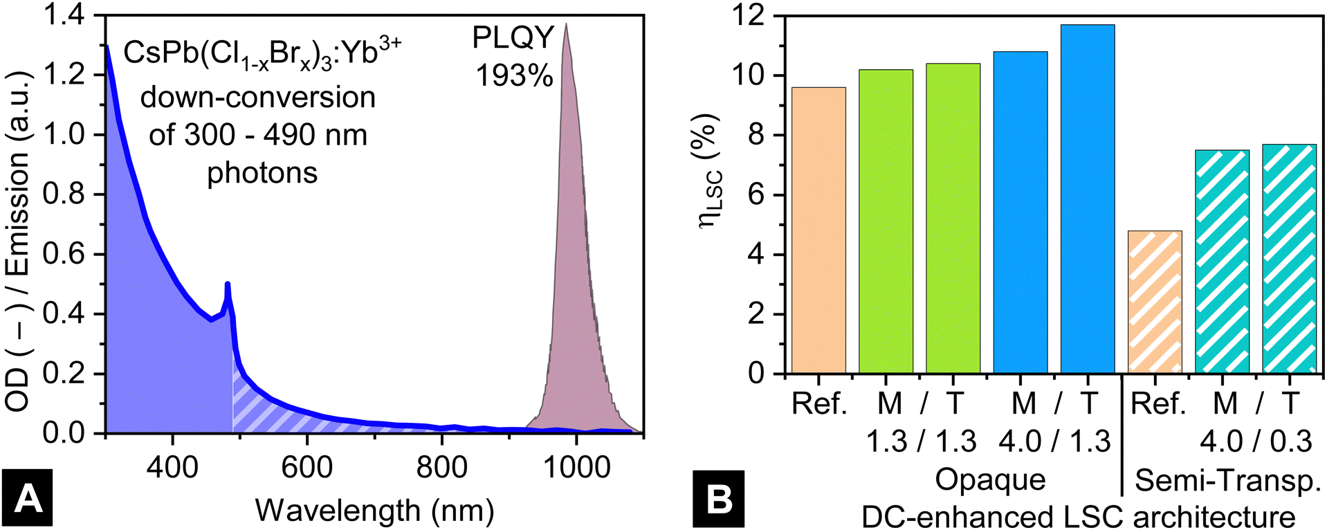
The possible application of (i) up-conversion (UC) and (ii) down-conversion (DC) – also referred to as quantum cutting – materials for enhancing the range of wavelengths of sunlight harvested has long been wished for.102,103 A photophysical analysis by Richards et al. has clearly indicated that >100 × -gains – in either the intermediate state lifetime of the lanthanide ions or the incident photon flux – would need to be made before UC would even start to become efficient for solar harvesting applications.104 While organic materials can exhibit significantly longer lifetimes and therefore offer more hope of UC working under one-sun concentrations, such materials are typically functioning only with visible light and tend to work much less efficiently when moving into the NIR.104 One avenue that might be possible is the introduction of microlens arrays above the LSC, such that an increased excitation intensity can be experience by the UC layer. However, the introduction of lenses goes against two of the original advantages of the LSC; that of being able to make full use of diffuse light and also not requiring solar tracking. Thus, the scope for UC to contribute in a meaningful way to LSC efficiencies is seen as very limited.With regard to DC, Gamelin and co-workers have presented exciting results over recent years relating to material with ∼190% PLQY based on a Yb3+-doped metal halide perovskite, CsPb(Cl1−xBrx)3.105 Unfortunately, the near-200% PLQY values are only achievable under low photon fluxes and once the photon flux is similar to that encountered under terrestrial sunlight the PLQY has already decreased to around 100%.61 It remains unclear whether strategies, such as increasing the Yb3+ concentration can circumvent the saturation issue.61 Indeed, researchers have implemented DC QDs into LSCs, with Luo et al. using Yb3+-doped CsPbCl3 NCs with a claimed PLQY of 164%.106
Here, an optimistic outlook is taken and it is assumed that this performance saturation at even moderate light intensities can be overcome to allow for near-200% DC to be realised. To evaluate the potential of DC to boost the LSC, in this sub-section the performance of adding a DC material – that of CsPb(Cl1−xBrx)3:Yb3+, which has a PLQY of 193% as reported by Kroupa et al.,105 the absorption and emission spectra of which are plotted in Fig. 13A – is evaluated. Given that the Yb3+ emission peaks are at 980 nm, conservation of energy dictates that the longest wavelength excitation photons that are able to contribute towards the 193% PLQY are at 490 nm. This means that the best performing LSC incorporating DC QDs should absorb all 300–490 nm light could be stack in tandem together with a a standard down-shifting QD LSC layer to harvest more of this visible & NIR photons.
 | ||
| Fig. 13 (A) Absorption and emission spectrum of the down-conversion material of CsPb(Cl1−xBrx)3:Yb3+, which is able to convert each short-wavelength (300–490 nm) photon into 1.93 NIR (980 nm) photons (as reported by Gamelin and co-workers105). Longer-wavelength (>490 nm) photons were assumed to exhibit a 100% PLQY. Here an OD = 1.3 is plotted. (B) A performance comparison of a variety of DC-enhanced commercial-scale (100000 cm2) LSCs in both opaque and semi-transparent configurations compared to their respective references (best-performing LSCs from Fig. 9C). For incorporating the DC material into the LSCs, two architectures are pursued: (i) the DC material was mixed (denoted as ‘M’) into the main QD layer or (ii) alternately as a tandem (denoted as ‘T’) structure, whereby the DC layer is placed on top of the standard QD-based LSC. Furthermore, the OD of the materials were varied: for the opaque LSCs (solid bars) the OD of DC material was either 1.3 or 4.0 (in addition to the standard QD-based LDS with OD = 1.3); whereas for the semi-transparent LSC a single OD of the DC material is partnered with the standard OD = 0.3 layer. | ||
In order to investigate this, the best-case commercial-scale opaque LSC from Fig. 9C above (OI* = 0.001, PLQY = 100%) with ηLSC = 9.6% is adopted as the reference device. For the first round of experiments, the concentration of DC material is chosen to be OD = 1.3 (see Fig. 13A) and is either: (i) mixed into the pre-existing QD-based LSC waveguide; or (ii) a double-layered tandem structure is created, whereby the DC material is contained in an additional overlying LSC layer, which is optically-coupled to the underlying down-shifting LSC as outlined above. This means that there is no air gap present between the differently doped layers. From Fig. 13B it can be seen that the mixed case (ηLSC = 10.2%) performs slightly worse than the tandem LSC (ηLSC = 10.4%). Both of these gains are lower than anticipated due to competition between the two luminescent species for absorbing the 300–490 nm photons, i.e. 300–490 nm photons that are absorbed by the down-shifting LSC layer are only going to emit with a maximum PLQY of 100%. This occurs regardless of which of the two architectures – (i) and (ii) above – are chosen. To overcome this such that light absorption into the DC QDs is favoured, the concentration of DC QDs was increased to OD = 4, allowing it to absorb 99.99% of short-wavelength light, while the underlying LSC remained at OD = 1.3 (opaque). Now, the tandem approach increases the maximum efficiency for this commercial-scale device up to 11.7%, a significant enhancement compared to the 9.6% single-layer reference LSC, while the mixed approach yields ηLSC = 10.8% – lower due to the fact that the is still competition between the two luminescent species for the same short-wavelength photons. Thus, as soon as the “photon bottleneck” issue is solved such that 200% PLQYs can be achieved under standard terrestrial sunlight, then an instant performance boost can be expected here. It should also be noted that the issue of the overlap integral also needs to be reconsidered in such configurations, given that both luminescent species are effectively in the same LSC layer. In the present example, this is not a problem given that the Yb3+-emission spectrum is very similar to the low-OI* (0.001) QDs emitting at 1000 nm that were used in from Fig. 9C above.
The same approach was also pursued for a semi-transparent LSC in both mixed and tandem architectures, building on the reference case from Fig. 9D above (best commercial-scale semi-transparent LSC, with OI* = 0.001, PLQY = 100% with ηLSC = 4.9%). From Fig. 13B (it can be seen that more significant gains can be made with either a mixed or tandem architecture, reaching ηLSC = 7.5% and ηLSC = 7.7%, thus representing a 53–57% enhancement. Both architectures exhibiting an AVT of 48%, demonstrating that via sacrificing the UV and blue factions of sunlight a significant enhancement in energy conversion can be achieved with only a slight reduction in AVT being incurred.
Furthermore, it is worth pointing out that the QD concentrations used (both 4.0 and 0.3) are retained in order to allow a clearer comparison with other results, rather than adjusting the AVT again. Overall, this result emphasises the potential of being able to semi-selectively harvest non-visible photons for the generation of electricity without trading this off directly against daylighting ability. Naturally, such a process would be boosted if NIR photons in the range 700–900 nm could also be efficiently harvested while still being emitted at an energy above the c-Si bandgap.
7.2 Issues relating to solar cells
Early on in the field of LSC development, it was acknowledged that the light intensity distribution across a square edge varied considerably. Friedman demonstrated that the luminescence intensity was constant near the centre of the LSC edge (central 30% region), and dropped off considerably to around half this value at the corners.32 The impact of this is that if multiple solar cells need to be connected in series to cover one entire LSC edge, then each solar cell will generate a different photocurrent and problems with current-matching will result. Wilson et al. investigated issue and, via adjusting the lengths of the strips of c-Si solar cells from 7.6 cm to 10.0 cm, achieved current matching and a 15% increase in power output.45 Of course, this problem can be entirely circumvented by moving to a circular LSC where the intensity distribution around the edge is equal in all directions. The bending radius of thin c-Si solar cells is not the problem here,107 however covering large areas (e.g. of a building) with a low packing density form such as a circle is likely not practical.A further issue addressed by Wilson et al. is that of designing the solar cell for a specific solar concentration. The c-Si solar cells were specifically designed to perform best at a solar concentration of 5 suns (i.e. 5-times higher photocurrent than under STC), which closely matched the final 4.8× concentration of the 60 cm × 60 cm LSC. The main consideration in the solar cell design is its ability to transport higher currents (I) at the lowest possible resistance, given that power losses due to series resistance (Rs) scale as I2Rs. While neither of these points are the biggest bottleneck in the technology at present, both will become more important as the LSC areas increase. It is also worth noting that further slight gains stand to be made given that the majority of solar cells used for LSCs exhibit an anti-reflection coating designed for AM1.5G sunlight. However, the much narrower bandwidth of the luminescence spectrum incident upon the edge-mounted solar cells (e.g. here ∼160 nm) means that an ARC exhibiting reflectance losses of <1% should be realisable in this range, thus possibly resulting in a ∼1% relative performance gain, as reported many decades ago by Garner et al.108
7.3 The role of rear reflectors
Previously, the addition of HMs for reducing ECL from via the front side was discussed. On the rear side, both specular and diffuse (Lambertian) reflectors can be utilised, but play different roles. In either case it is essential to maintain an air gap to the LSC waveguide, such that TIR is not disrupted (as was shown earlier in Fig. 12A). Specular reflectors are primarily employed on the rear when a double-pass of the incoming light would result in increased absorption by the LSC.109 This enables a lower QD concentration to be used whilst still maintaining, or even improving, overall LSC performance, given that the lower concentration of QDs will also result in a slight reduction in re-absorption (and hence fractionally lower ECL).Lambertian reflectors have been used in many of the highest-efficiency LSCs to date, playing a number of possible roles. The first is the same as described above as for the specular reflector, whereby short-wavelength light is given another opportunity to be absorbed. An example of this was presented above, where stripes of doped LSC material relied on a white rear scattering layer to achieve significant absorption of the solar spectrum.94 Secondly, small-area LSCs exhibit the ability of the edge-mounted solar cells in the waveguide to simply collect sunlight scattered off the rear. This effect can only work in small-area devices since if sunlight is scattered in air (n = 1) and enters the rear of a waveguide slab with n ∼ 1.5 then – via the reciprocity of light – it cannot undergo TIR off the front air:waveguide interface. Thus, the scattered light must reach the edge within its first pass through the waveguide, otherwise it is lost. This effect is most pronounced for longer-wavelength light that cannot be absorbed by the LSC and is typically regarded as an edge-effect by the LSC community.92,110 While this has resulted in some thoughts about the potential of a “scattering solar concentrator”, it was pointed out several decades ago that such a scattering concentrator would be bound by the 2n2 limit.111,112
The use of reflectors with LSCs come at a price. Given that air gaps must to be maintained between the waveguide and the mirror(s), the LSC is no longer a single slab of material and now either: (i) small spacers are required during LSC assembly, which both disrupt TIR and alter the uniform aesthetics of the LSC, given that these points of optical contact are going to out-scatter light; or (ii) the edge mounting frame needs to be modified to hold two sheets, such as is the case with double glazing (discussed further in the economics section below). Perhaps a more obvious disadvantage is that the LSC cannot be used as a building element that allows daylighting anymore – the LSC is likely no longer transparent and this will also prevent the LSC from harvesting any light (e.g. room light) incident from the rear side.
The final place where mirrors have been used in LSCs is along the edges. The original motivation of this in the late 1970s/early 1980s was due to the high cost of the c-Si solar cells and the cost of evaporating a metal reflector along the edge of the waveguide was cheaper.8 Indeed, this was one motivation for triangular LSC originally proposed by Goetzberger and Greubel, with a metal reflector coated onto the hypotenuse.8 Cost issues aside, such a one-edge coated LSC is expected to perform significantly worse than a square one having all four edges coated due to the longer optical pathlengths in the former case, which naturally only increase the probability of losses. Recently, Bernardoni et al. reported using a highly reflective polymeric foil (3M DF2000MA) along edges of the LSC where no PV devices were mounted.35
7.4 Performance under diffuse light and shading resistance
The performance of LSCs has been claimed to be more efficient under cloudy skies,34 however such claims and the evidence behind them need to be understood carefully. Firstly, it is important to remember that the solar irradiance spectrum on a cloudy day exhibits a slight blue shift in the average photon energy, as well as a significant reduction in intensity.113 Thus, any solar energy harvesting technology that exhibits a higher bandgap – whether this be an amorphous silicon solar cell or the dyes used within a LSC34 – can exhibit a higher efficiency under overcast conditions compared to that under direct sunlight (STC conditions). However, even though the efficiency of these devices might be fractionally higher under diffuse illumination, one should not forget that the absolute amount of power generated could still be significantly lower than a standard c-Si flat-plate PV module.114 The second reason for a LSC exhibiting improved performance under cloudy skies relates to its mounting angle. If the LSC is vertically-mounted then it is able to accept incident light from both sides of the panel, like any other bifacial PV technology.115 Thus, diffuse light can be incident upon the LSC directly or it can be reflected from the ground (assuming non-zero albedo) before striking the panel.116 While testing a LSC in a vertically-mounted position might initially appear sensible given its potential for BPIV, it is then unlikely that any significant fraction of light will be incident upon the rear side when integrated into a building – at most typically room light, unless the LSC is integrated into the railing of a balcony, for example. Also, it should be noted that just because additional power is generated from the LSC when illuminated from both sides this does not per se convey an increase in efficiency. A similar debate has surrounded the power and energy rating of bifacial c-Si PV modules for more than a decade now, however no IEC standard has been adopted yet.117 With regard to LSCs, the issue of overestimation of LSC performance is discussed – and correct experimental approaches given – in the work by Lunt and co-workers.76Finally, there have been some preliminary reports that LSCs might also exhibit increased shading resistance as opposed to standard flat-plate PV modules.118 In classical c-Si or thin-film PV modules, shading – a severe case of which can be imagined as the shadow of a pole passing across a module – can result in near-zero photocurrent generation in one cell. Even if this is shading a relatively small area of the entire PV module, the series-connected nature of the solar cells leads to the one shaded cell creating a bottleneck to the flow of current in the entire string. This is less likely to occur in a LSC since even if the area around one of the edge-mounted solar cells is shaded, this solar cell will still receive luminescence generated from other areas of the module. The effect of shading in flat-plate PV modules is traditionally mitigated via the inclusion of bypass diodes, and while have also been experimented with in LSC modules15 such solutions need to be optimised upon commercialisation of the technology.
8. Financial considerations
At the time when the LSC technology was originally proposed, fabricating c-Si solar cells was an expensive exercise, costing around 25 € per W73 in 1980–1985. Given that such costs were significantly higher than those for optical elements or waveguide materials (based on glasses or polymers), all CPV technologies were an interesting economic proposition at the time. Over the years though, the cost of producing c-Si devices has steadily declined, while at the same time efficiencies have increased, resulting in costs today of about 0.14–0.18 € per W for high efficiency c-Si solar cells and 0.24–0.26 € per W for c-Si PV modules.73,74 Before considering the economics of the LSC technology further, the most likely choices for the key components are briefly discussed:(i) Waveguide material: neither quartz/fused silica nor optical-quality glasses such as N-BK7 are available in a large-area format. This leaves the highest quality float glasses as the best alternative, such as Schott Borofloat borosilicate glass that could cost 60 € per m2 in full-scale production.119 Although the attenuation coefficient at α ∼ 10−2 cm−1 is higher than some polymers, the scope for implementing large sheets of flammable polymers in buildings is problematic from a fire resistance point of view54 – possibly the only chance being via a triple-glazed unit containing glass/polymer/glass panes.
(ii) Luminescent material: this work considers LSCs based on QDs. Jean et al. determined that the costs for synthesizing lead sulphide (PbS) and metal halide perovskite (CsPbI3) QDs today are prohibitively high, with median costs of 10–52 € per g1 and 64 € per g1, respectively.120 For fabricating a LSC technology the cost of a 500 nm thick film (deposited via slot-die coating) of these QD absorbers per area has been estimated to be ∼46 € per m2 (PbS) and ∼150 € per m2 (CsPbI3).120 In the QD solar cells investigated by Jean et al., the QD materials alone comprised up to 55% of the total module cost, which ranged from 0.13–0.74 € per W (PbS) and 0.64 € per W (CsPbI3) assuming a 20% efficient cell.120 In comparison, bulk quantities of fluorescent organic dyes – for example, the commonly used BASF Lumogen perylene-based dyes – cost 7–9 € per g1,121 roughly an order of magnitude cheaper than the cost of QDs today, but naturally also having benefitted from economies-of-scale such that they are now synthesized in 50 kg batches.
(iii) Choice of host material: past research has indicated that fluorinated polyurethane (for example, Lumiflon LF-910LM) could be a promising host for LSCs considering its: (i) compatibility with luminescent materials, such as Lumogen dyes;50,122 (ii) 30 years stability guarantee;123 and (iii) relatively low costs for a fluorinated polymer at ∼35 € per m2.124 The latter price is based on a 25 μm layer thickness and even though the application was very different (part of a corrosion resistant layer stack for steel bridges124), it is very similar to the 30 μm layers successfully used for LSC-pumped solar lasers.125
(iv) Solar cells: as described in Section 2 (LSC Simulation Framework), the highest efficiency c-Si solar cells were selected for edge attachment. These 26.7% efficient devices are assumed to be cut into long strips that are 0.3 cm wide, thus a 1 m2 LSC will require 120 cm2 (0.012 m2) of solar cells to cover all four edges. If the solar cells are assumed to cost 0.14 € per W,73,74 then this equates to a cost of only 0.45 € to cover the entire LSC perimeter (at a per area cost of 37.4 € per m2), which is negligible. This indicates that the suggestion of replacing cells on large-area LSCs with mirrors instead to save on costs8,35 as not being a fruitful direction in today's marketplace. It should be noted that it is assumed here that the efficiency of the solar cell can be maintained, even when cut into a 0.3 cm-wide strip. In reality, this would require an edge passivation strategy to be implemented in the device design – as developed by SunPower for 2.3 mm × 2.3 mm micro-concentrator solar cells126 – to avoid excessive recombination of electrons or holes at the edges of the solar cell.
(v) Encapsulation of solar cells: compared to classical flat-plate PV modules, the issue of encapsulating the solar cells to prevent the ingress of water and water vapour could be easier since the edge-mounted solar cells would be inside a frame, assumedly made of aluminium. A thick enough layer of the encapsulant between the solar cells and the LSC waveguide is needed to cope with thermal expansion issues. For example, the cyanoacrylate adhesive used by Wilson on a 60 cm × 60 cm LSC resulted in cracking and delamination upon full illumination under a solar simulator.119 Also, it is apparent that a dedicated machine – to laminate the solar cells to the edge of the LSC waveguide, interconnect these, and then encapsulate the edge inside a frame – needs to be developed, however there appears to be no technological barrier to achieving this. From the previously cited work by Jean et al., encapsulation in their devices contributed ∼50 € per m2 to the final module cost.120 A previous c-Si PV technology – called Sliver since it was based on mm-wide narrow devices – also relied on pick-and-place technology for module assembly, with Blakers et al. estimating the module assembly and encapsulation would cost ∼100 € per m2.127 Given that the cost of encapsulation is already discussed above, it could be assumed that 50 € per m2 would be sufficient for solar cell attachment and interconnection costs.
(vi) Installation: if the LSC is mounted into a window frame and becomes an electrically-active window, this will require a mind-shift with installers as well. For example, the window installer now needs to be an electrician as well (or work as a close team), however this appears to be an initial teething problem that would be solved with market growth (window installation is discussed more below).
(vii) Transparency: many LSC papers feature transparency as an advantage, however it is obvious that a 50% transparent LSC module is going to exhibit nearly double the € per W cost compared to a fully opaque LSC – since only slight savings in the amount of luminescent materials can be made and all other module expenses and balance-of-systems costs remain the same.
(viii) Stability: flat-plate c-Si PV modules have steadily demonstrated increased reliability in the field, with some manufacturers now giving up to 30 years guarantee that the PV module will still deliver 80–90% of its original rated power. It was indicated above that a fluoropolymer host can last for this duration, thus the stability of the perovskite QDs themselves is the current weak link, as recently reviewed by Yuan et al. for photovoltaic devices.128 However, QDs are widely used in optoelectronic devices today including large-area displays and some of the potential approaches that have been applied to other QD systems (see Moon et al. for a recent review129) could also benefit the performance of QDs for LSCs.
Does this mean that the LSC technology will remain within the realm of architects and high-end demonstration projects? Maybe not, since it cannot be denied that the cost of architectural glazing is already high and, naturally, such a window does not generate any electricity. Values extracted from the work of Kralj et al.130 indicate that a triple-glazed unit can cost from 108 € per m2 up to 690 € per m2, with framing, transportation and installation an additional 170–420 € per m2. In these prices, the cost of the intermediate glass pane contributes is very low at 10 € per m2. Thus, a realistic starting point is to assume that this middle pane is replaced by the active LSC waveguide, in this case chosen to be highly transparent glass. All of the above estimations are now summarised in Table 3. This indicates that the active LSC waveguide based on NIR QDs is expected to cost 255–355 € per m2, which then needs to be added to the remainder of the triple-glazed unit – bringing up the cost to 355–1035 € per m2 – while finally framing, transport and installation create an installed system cost of 525–1455 € per m2. While it might be tempting to make a direct comparison to the module costs for c-Si flat-plate PV, it is worth remembering that such a triple-glazed window element exhibits a heat transfer coefficient, or U-value, of 0.9–1.1 W m−2 K and is probably now best regarded as a combined photovoltaic/thermal (PV/T) module.
| Large-area LSC unit | Cost (€ per m2) | Ref. |
|---|---|---|
| a Cost derived from 100 € per m2 cost for module assembly from Blakers et al.,127 with the encapsulation component removed. | ||
| Triple-glazed window unit (minus middle pane) | 100–680 | 130 |
| QD LSC – active middle pane: | ||
| Glass waveguide | 60 | 119 |
| NIR QDs | 50–150 | 120 |
| Fluoropolymer host | 35 | 124 |
| Attaching & interconnecting solar cells | 50a | 127 |
| Encapsulation | 50 | 120 |
| Junction box & cables | 10 | 120 |
| Sub-total QD LSC middle pane: | 255–355 | (This work) |
| Sub-total triple-glazed QD LSC unit: | 355–1035 | (This work) |
| Framing | 80–200 | 130 |
| Transportation (1000 km) | 10–20 | 130 |
| Installation | 80–200 | 130 |
| Total installed triple-glazed QD LSC unit: | 525–1455 | (This work) |
Regarding the performance of such a LSC unit, the extra layer of external glazing will incur an additional ∼8% reflectance loss due to the inclusion of an additional n = 1.5 layer being placed in front of the LSC. Based on the best-performing commercial-scale opaque LSC, this would reduce the performance from ηLSC = 9.6% down to ηLSC = 8.8%, thus resulting in a LSC unit that can yield 88 W m−2. This indicates that a triple-glazed QD LSC unit (355–1035 € per m2) yields a module price of 4.0–11.8 € per W. This is similar to a recent cost estimate for medium-area (25 cm × 25 cm) LSCs, which ranged from 7–13 € per W (depending on the number of edges coated with solar cells) and were based on organic dyes and exhibited efficiencies in the range of 1.6–1.9%.35 These costings are also in line with figures published for BIPV solar façade costing about 600 € per m2, costing 340 € per m2 more than a non-PV equipped façade.131 It should be noted that specialised architectural cladding options such as high quality stone or glass curtain walls can cost 400–600 € per m2 and 500–1100 € per m2,131 respectively.
From this estimate it is now relatively easy to determine what a semi-transparent triple-glazed LSC unit would cost. For example, assuming an AVT of 50% results in a power output of 44 W m−2 and the cost of QDs being halved – but also other components remaining at the same price – amounting to 8.1–23.5 € per W. Having these values enables the architect/installer/owner to make an informed decision based on the electrical, daylighting and thermal performance of such a triple-glazed LSC unit.
9. Outlook
From this work, the following efficiency targets for opaque LSCs are suggested for three common sizes:• Lab-scale LSCs (25 cm2): target ηLSC is 11.0% and 5.5% for opaque and semi-transparent LSC modules, respectively. The best result reported in this is size category is ηLSC = 7.1% – an opaque device benefitting from GaAs solar cells and a diffuse rear reflector43 – indicating even that lab-scale devices have a way to go before reaching the desired target efficiency.
• Pilot-scale LSCs (1000 cm2): target ηLSC is 10.0% and 5.0% for opaque and semi-transparent LSC modules, respectively. Towards meeting this goal, the 6.8% result of Anand et al. for a 900 cm2 LSC is impressive, however it should be noted that this is the optical power efficiency,41i.e. no optical-to-electrical energy conversion has taken place.
• Commercial-scale LSCs (100000 cm2): target ηLSC is 9.0% and 4.5% for opaque and semi-transparent LSC modules, respectively. To date, no LSCs of this size have been produced, with the reported efficiencies of the largest (LSC areas of 2500–7400 cm2) being in the range ηLSC = 0.3–1.6%.45–47 Thus, this efficiency target appears to be extremely challenging, mostly due to the very stringent demands on the overlap integral for large-area LSCs as illustrated in Fig. 9C and D.
If the LSC efficiencies remain too low, two possible approaches could be pursued. The first, simulated by Aghaei et al. suggests arranging smaller cubes of LSCs into an array with bifacial c-Si solar cells in between them,132 although scale-up on this approach and especially solar cell interconnections look tricky to solve and it is doubtful as to whether any concentration of sunlight actually occurs. However, the same approach has been experimentally demonstrated by Aste et al. whereby 50 cm × 50 cm plates (sub-modules) were assembled to realise a LSC with overall dimensions of 150 cm × 100 cm (ηLSC = 1.6%).46 The second approach would be to follow the idea suggested by Yang et al. and place micro-solar cells on the rear of the LSC waveguide.75 Once solar cells start occupying an increasing area on the rear of the LSC module, it starts approaching a luminescent down-shifting (LDS) technology instead. While the differences between such configurations – i.e. rear-mounted cells in a LSC versus sparsely-mounted cells in a LDS module – are small, it is worth remembering that the original goal of the LDS technology was to overcome the poor short wavelength EQE of solar cells and not as a concentrating PV or daylighting technology. While LDS has been successfully applied to both mini-modules of c-Si, CIGS and cadmium telluride (CdTe)133 as well as full-size CdTe modules (120 cm × 60 cm),134 it has not found its way into production yet. The costs of such an approach relying on the use of micro solar cells will ultimately depend on the economies-of-scale of production and (likely) the implementation of pick-and-place machines, which been experimented with for the laying-out of small-area c-Si solar cells.135
It also has to be noted that classical flat-plate c-Si PV modules achieved long-term success primarily via economies of scale and continued improvements to the technology. Specifically the learning curve for c-Si PV has demonstrated that in the last four decades the price decreased by 24% with each doubling of the cumulative module production.73 Currently, there appears to be no data for a BIPV learning curve, and if every building is different how do BIPV technologies escape from being confined to demonstration projects? From a recent survey of architects, while aesthetics was the most important consideration overall, several interviewees indicated that transparency and/or colour was only desired as long as no sacrifice in technical performance had to be made136 – a tough ask!
While the immediate challenges facing the LSC technology achieving higher efficiencies on larger areas, further challenges facing the technology in the future will be stability – including stability under sunlight as well as to moisture and temperature – as well as concepts for attaching and encapsulating the solar cells on the LSC perimeter. Furthermore, if architects and window manufacturers/installers are to adopt this new technology, then many new aspects need to be considered. For example, is the waveguide made of a polymer? If so, does it satisfy national building and fire regulations? What needs to be considered for the installation of industrial window frames since they will now have electrical connections within them. An example of using standard industrial framing for double-glazed commercial windows to house two 30 cm × 30 cm PMMA-based LSCs is illustrated in Fig. 14. This early prototype exhibited a low efficiency (ηLSC = 0.2%) and a moderate thermal resistivity (U-value) of 2.3 W m−2 K−1.137
 | ||
| Fig. 14 (A) The double-glazed LSC system with c-Si PV cells attached and wired to primary LSC waveguide. (B) Empty curtain wall frame. (C) Front view of assembled double-glaze LSC system (from outside building). (D) Assembled double-glaze LSC system from what would be an internal view looking out. | ||
With regard to semi-transparent devices, only time will tell as to whether a power-generating window technology that can generate 44 W m−2 for an additional outlay of 255–355 € per m2 compared to a standard triple-glazed unit remains an attractive proposition. As a final note, it will not surprise any reader to learn that an aluminium-framed triple-glazed window not only generates no electricity, but in fact consumes a huge amount of energy during its fabrication, recently reported to be on average 534 kW h m−2 by Asdrubali et al.138 Thus, on the one hand, even a LSC exhibiting a low ηLSC is likely to make a positive impact here. However, on the other hand, the energy payback time (EPBT) – defined as the amount of time that a solar panel takes to generated the amount of energy that went into its manufacture139 – is likely to be long. To evaluate this, a simple evaluation of a commercial-scale semi-transparent LSC with ηLSC = 4.4% (44 W m−2) was conducted using PVGIS, an online PV performance tool.140 The LSC module was assumed to be installed vertically on a south-facing building in Karlsruhe, Germany. The annual electricity production of this LSC module is 52 kW h m−2, resulting in a EPBT of ∼13 years, which is roughly 10-times longer than for a flat-plate c-Si PV module (EPBT ∼ 1.3 years in a similar location73). Now that the annual performance of a large-area LSC has been estimated, it is possible to go one step further and – taking an average installed LSC price of 990 € per m2 from Table 3 above and assuming a system lifetime of 40 years and 2% inflation – the levelized cost of electricity (LCOE) from the semi-transparent LSC module in Karlsruhe is determined to be €1.47 per kW per h. Again, this is ∼€1.4 per kW per h higher than the LCOE of generating solar electricity from a flat-plate c-Si PV system, however it is worth highlighting that both the LCOE and EPBT are, of course, infinitely better than a standard triple-glazed window!
10. Conclusions
Many factors can limit the performance of a LSC for the generation of solar electric power. Naturally, it is important to absorb the widest possible bandwidth of sunlight that still enables emission at a wavelength above the bandgap of the edge-mounted c-Si solar cells. The optimum here was determined to lie in a broad range, both in terms of wavelength (950–1000 nm peak) and OD (0.6–1.0). Not surprisingly, the LSC performance scales linearly with the PLQY of the QD emitters.Luminescence that does not reach the edges of the LSC is the key reason for poor performance and low ηLSC. It was determined that LSCs remain surprisingly tolerant to even moderate amounts of host attenuation (up to 10−2 cm−1) with only small reductions in performance being observed. In this review, the issue of scale-up is focussed on and the link back to materials requirements made. For example, while an OI* value of 0.019 is sufficient to achieve a conversion efficiency to ηLSC = 12% in an opaque lab-scale (25 cm2) LSC, the same degree of spectral overlap limits a commercial-scale (100000 cm2) LSC to be only ∼1% efficient. However, by employing a QD that exhibited a greatly reduced OI* (<0.001), an opaque commercial-scale LSC could indeed exhibit much better performance of ηLSC = 9%. The degree of OI* was demonstrated to dramatically increase the ECLs, thus reducing the waveguiding efficiency. It is demonstrated that if materials scientists can achieve OI* < 0.001 in a NIR-emitting luminescent material on a pilot-scale device then the greatest barriers are overcome for scaling this up further to a commercial-scale LSC. With regard to semi-transparent LSCs many of the same trends exist as in the opaque case, however sometimes the design constraints are relaxed somewhat (but not significantly).
The effect of re-absorption is examined in great detail, for example, with regard to absorption tails that are known to be a problem both in dye-based and QD-based LSCs. This again emphasises the importance on designing QD systems that exhibit a near-zero OI* between the absorption and emission spectra. Alternatively, various novel approaches are reviewed for minimising ECLs including the use of hot-mirrors, spatial variation of the luminescent material, or even alignment of some luminescent species (such as organic dyes), however each of these approaches also bring drawbacks. Boosting LSC performance via UC appears to be very limited, however the rapid progress made in DC materials over the last few years suggests that sizable gains could be made there once such materials are either mixed in with other QDs or indeed stacked in a tandem configuration. In particular, the gains for semi-transparent LSCs is great, resulting in a possible >50% enhancement in ηLSC.
Thus, many of the challenges in achieving high efficiencies only appear once at least pilot-scale (1000 cm2) LSCs are attempted. For this reason, three efficiency threshold targets for opaque LSCs are recommended in order to create a pathway to success: lab-scale (25 cm2) ηLSC = 11% for opaque and 5.5% for semi-transparent, since such dimensions are easy to produce in many labs around the world via many different fabrication techniques; pilot-scale (1000 cm2) ηLSC = 10% for opaque and 5% for semi-transparent, since the results of this study demonstrate that the materials requirements become critical to reach these goals; and commercial-scale (100000 cm2) ηLSC = 9% for opaque and 4.5% for semi-transparent, since this is the same order of magnitude as large panes of architectural glass.
Many non-technical issues for LSCs also remain to be overcome before their penetration into the BIPV market can be ensured. The installed cost of a modified triple-glazing unit where the centre pane is swapped with a LSC waveguide was calculated. The active LSC pane alone costs between 255–355 € per m2 when based on the use of perovskite QDs, while the remainder of the triple-glazing unit is more variable at 100–680 € per m2, making a total of 355–1035 € per m2, for the triple-glazed LSC unit. A yield of 88 W m−2 is possible with an opaque LSC, from which a LSC module price of 4.0–11.8 € per W can be derived, which is 15–50 times the current price of a c-Si PV flat-plate PV module. A semi-transparent exhibiting an AVT of 50% will yield roughly half the electrical power output, but nearly all components in their construction will remain the same, with only a slightly lower concentrations of QDs being required. This suggest that a semi-transparent LSC module will cost 8.1–23.5 € per W. While prices can be expected to go down as sales increase and production volume grows, this will not occur if the LSC technology does not break out of its present demonstrator-status as a technology. In addition, challenges remain to ensure that LSC units that are deployed into the cladding of buildings are compatible lifetime-wise as well as with national fire codes and building regulations.
However – like many renewable energy solutions that are needed to power systems in different geographic locations around the world – it is possible that the LSC will be a complementary technology in the world of semi-transparent photovoltaics. This will happen when the low-hanging fruit – i.e. putting opaque c-Si PV in the easy parts of the building – have all been picked and we are encouraged to seek solutions for BIPV facades (with AVT of 50%) along with agrivoltaics – the use of PV within agriculture – and vehicle-integrated PV.
Conflicts of interest
There are no conflicts to declare.Acknowledgements
BSR gratefully acknowledges the financial support from the Helmholtz Association, including (i) a Professorial Recruitment Initiative; and (ii) the Helmholtz-Program MTET (Materials and Technologies for the Energy Transition) – Topic 1 Photovoltaics (38.01.05).References
- European Commission, Fact Sheet: Making our homes and buildings fit for a greener future, 2021, https://ec.europa.eu/commission/presscorner/api/files/attachment/870607/Factsheet%20Buildings_EN.pdf.
- The European Parliament and the Council of the European Union, Official Journal of the European Union, 2010, L153, 13–35 Search PubMed.
- European Commission, European Green Deal: Commission proposes to boost renovation and decarbonisation of buildings, 2021, https://ec.europa.eu/commission/presscorner/api/files/document/print/en/ip_21_6683/IP_21_6683_EN.pdf.
- Technavio, Building Integrated Photovoltaics Market by End-user, Panel Type, and Geography – Forecast and Analysis 2021–2025, 2021, https://www.technavio.com/report/building-integrated-photovoltaics-market-industry-analysis.
- T. E. Kuhn, C. Erban, M. Heinrich, J. Eisenlohr, F. Ensslen and D. H. Neuhaus, Energy Build., 2020, 110381 Search PubMed.
- W. Celadyn and P. Filipek, Buildings, 2020, 10, 145 CrossRef.
- C. Xiang, P. Green and B. S. Matusiak, Color Res. Appl., 2021, 46, 524–537 CrossRef.
- A. Goetzberger and W. Greubel, Appl. Phys., 1977, 14, 123–139 CAS.
- W. H. Weber and J. Lambe, Appl. Opt., 1976, 15, 2299–2300 CrossRef CAS PubMed.
- A. A. Earp, G. B. Smith, J. Franklin and P. Swift, Sol. Energy Mater. Sol. Cells, 2004, 84, 411–426 CrossRef CAS.
- E. P. Merkx and E. van der Kolk, Indoor Photovoltaics: Materials, Modeling and Applications, 2020, pp. 133–188 Search PubMed.
- J. A. H. P. Sol, G. H. Timmermans, A. J. van Breugel, A. P. H. J. Schenning and M. G. Debije, Adv. Energy Mater., 2018, 8, 1702922 CrossRef.
- Á. Bognár, S. Kusnadi, L. H. Slooff, C. Tzikas, R. C. Loonen, M. M. de Jong, J. L. Hensen and M. G. Debije, Renewable Energy, 2020, 151, 1141–1149 CrossRef.
- A. Kerrouche, D. A. Hardy, D. Ross and B. S. Richards, Sol. Energy Mater. Sol. Cells, 2014, 122, 99–106 CrossRef CAS.
- W. van Sark, P. Moraitis, C. Aalberts, M. Drent, T. Grasso, Y. L'Ortije, M. Visschers, M. Westra, R. Plas and W. Planje, Solar RRL, 2017, 1, 1600015 CrossRef.
- A. Renny, C. Yang, R. Anthony and R. R. Lunt, J. Chem. Educ., 2018, 95, 1161–1166 CrossRef CAS.
- C. Corrado, S. W. Leow, M. Osborn, I. Carbone, K. Hellier, M. Short, G. Alers and S. A. Carter, J. Renewable Sustainable Energy, 2016, 8, 043502 CrossRef.
- T. Masuda, M. Iyoda, Y. Yasumatsu, S. Dottermusch, I. A. Howard, B. S. Richards, J.-F. Bisson and M. Endo, Commun. Phys., 2020, 3, 1–6 CrossRef.
- D. Cambié, J. Dobbelaar, P. Riente, J. Vanderspikken, C. Shen, P. H. Seeberger, K. Gilmore, M. G. Debije and T. Noël, Angew. Chem., 2019, 131, 14512–14516 CrossRef.
- S. F. Mohsenpour, B. Richards and N. Willoughby, Bioresour. Technol., 2012, 125, 75–81 CrossRef CAS PubMed.
- W. Stahl, V. Wittwer and A. Goetzberger, Sol. Energy, 1986, 36, 27–35 CrossRef CAS.
- M. Portnoi, P. A. Haigh, T. J. Macdonald, F. Ambroz, I. P. Parkin, I. Darwazeh and I. Papakonstantinou, Light: Sci. Appl., 2021, 10, 3 CrossRef CAS PubMed.
- I. Papakonstantinou, M. Portnoi and M. G. Debije, Adv. Energy Mater., 2021, 11, 2002883 CrossRef CAS.
- J. Roncali, Adv. Energy Mater., 2020, 10, 2001907 CrossRef CAS.
- Y. Zhou, H. Zhao, D. Ma and F. Rosei, Chem. Soc. Rev., 2018, 47, 5866–5890 RSC.
- H. Hernandez-Noyola, D. H. Potterveld, R. J. Holt and S. B. Darling, Energy Environ. Sci., 2012, 5, 5798–5802 RSC.
- Z. Mi, J. Chen, N. Chen, Y. Bai, R. Fu and H. Liu, Energy Convers. Manage., 2016, 117, 142–149 CrossRef.
- G. Smestad, H. Ries, R. Winston and E. Yablonovitch, Sol. Energy Mater., 1990, 21, 99–111 CrossRef CAS.
- E. Yablonovitch, J. Opt. Soc. Am., 1980, 70, 1362–1363 CrossRef.
- T. Huld, R. Müller and A. Gambardella, Sol. Energy, 2012, 86, 1803–1815 CrossRef.
- V. Wittwer, W. Stahl and A. Goetzberger, Sol. Energy Mater., 1984, 11, 187–197 CrossRef CAS.
- P. S. Friedman, Opt. Eng., 1981, 20, 206887 Search PubMed.
- D. Alonso-Alvarez, E. Klampaftis, D. Ross and B. S. Richards, IEEE J. Photovolt., 2014, 4, 1532–1537 Search PubMed.
- M. G. Debije and V. A. Rajkumar, Sol. Energy, 2015, 122, 334–340 CrossRef.
- P. Bernardoni, G. Mangherini, M. Gjestila, A. Andreoli and D. Vincenzi, Energies, 2021, 14, 816 CrossRef CAS.
- A. Reinders, R. Kishore, L. Slooff and W. Eggink, Jpn. J. Appl. Phys., 2018, 57, 08RD10 CrossRef.
- F. Meinardi, F. Bruni and S. Brovelli, Nat. Rev. Mater., 2017, 2, 17072 CrossRef CAS.
- Y. Zhao and R. R. Lunt, Adv. Energy Mater., 2013, 3, 1143–1148 CrossRef CAS.
- S. Mattiello, A. Sanzone, F. Bruni, M. Gandini, V. Pinchetti, A. Monguzzi, I. Facchinetti, R. Ruffo, F. Meinardi and G. Mattioli, Joule, 2020, 4, 1988–2003 CrossRef CAS.
- C. Yang and R. R. Lunt, Adv. Opt. Mater., 2017, 5, 1600851 CrossRef.
- A. Anand, M. L. Zaffalon, G. Gariano, A. Camellini, M. Gandini, R. Brescia, C. Capitani, F. Bruni, V. Pinchetti and M. Zavelani-Rossi, Adv. Funct. Mater., 2020, 30, 1906629 CrossRef CAS.
- M. G. Debije, R. C. Evans and G. Griffini, Energy Environ. Sci., 2021, 14, 293–301 RSC.
- L. H. Slooff, E. E. Bende, A. R. Burgers, T. Budel, M. Pravettoni, R. P. Kenny, E. D. Dunlop and A. Büchtemann, Phys. Status Solidi RRL, 2008, 2, 257–259 CrossRef CAS.
- C. Yang, M. C. Barr and R. R. Lunt, Phys. Rev. Appl., 2022, 17, 034054 CrossRef CAS.
- L. R. Wilson, E. Klampaftis and B. S. Richards, IEEE J. Photovolt., 2017, 7, 802–809 Search PubMed.
- N. Aste, L. C. Tagliabue, C. Del Pero, D. Testa and R. Fusco, Renewable Energy, 2015, 76, 330–337 CrossRef.
- J. Zhang, M. Wang, Y. Zhang, H. He, W. Xie, M. Yang, J. Ding, J. Bao, S. Sun and C. Gao, Sol. Energy, 2015, 117, 260–267 CrossRef CAS.
- K. R. McIntosh, N. Yamada and B. S. Richards, Appl. Phys. B, 2007, 88, 285–290 CrossRef CAS.
- S. F. Correia, P. P. Lima, P. S. André, M. R. S. Ferreira and L. A. D. Carlos, Sol. Energy Mater. Sol. Cells, 2015, 138, 51–57 CrossRef CAS.
- S. Dottermusch, T. Masuda, M. Endo, B. S. Richards and I. A. Howard, Adv. Opt. Mater., 2021, 9, 2100479 CrossRef CAS.
- B. S. Richards and K. R. McIntosh, Prog. Photovoltaics Res. Appl., 2007, 15, 27–34 CrossRef CAS.
- J. Huang, J. Zhou, E. Jungstedt, A. Samanta, J. Linnros, L. A. Berglund and I. Sychugov, ACS Photonics, 2022, 9, 2499–2509 CrossRef CAS.
- E. D. Palik, Handbook of Optical Constants of Solids, Academic Press, London, U.K., 1985 Search PubMed.
- M. Zettl, O. Mayer, E. Klampaftis and B. S. Richards, Energy Technol., 2017, 5, 1037–1044 CrossRef.
- P. Uprety, M. M. Junda and N. J. Podraza, Surf. Sci. Spectra, 2017, 24, 026003 CrossRef.
- J. C. Goldschmidt, M. Peters, A. Bösch, H. Helmers, F. Dimroth, S. W. Glunz and G. Willeke, Sol. Energy Mater. Sol. Cells, 2009, 93, 176–182 CrossRef CAS.
- R. Reisfeld, J. Less-Common Met., 1983, 93, 243–251 CrossRef CAS.
- O. Moudam, B. C. Rowan, M. Alamiry, P. Richardson, B. S. Richards, A. C. Jones and N. Robertson, Chem. Commun., 2009, 6649–6651 RSC.
- T. Wang, J. Zhang, W. Ma, Y. Luo, L. Wang, Z. Hu, W. Wu, X. Wang, G. Zou and Q. Zhang, Sol. Energy, 2011, 85, 2571–2579 CrossRef CAS.
- C. L. Mulder, L. Theogarajan, M. Currie, J. K. Mapel, M. A. Baldo, M. Vaughn, P. Willard, B. D. Bruce, M. W. Moss, C. E. McLain and J. P. Morseman, Adv. Mater., 2009, 21, 3181–3185 CrossRef CAS.
- C. S. Erickson, L. R. Bradshaw, S. McDowall, J. D. Gilbertson, D. R. Gamelin and D. L. Patrick, ACS Nano, 2014, 8, 3461–3467 CrossRef CAS PubMed.
- K. Barnham, J. L. Marques, J. Hassard and P. O’Brien, Appl. Phys. Lett., 2000, 76, 1197–1199 CrossRef CAS.
- Z. Li, A. Johnston, M. Wei, M. I. Saidaminov, J. M. de Pina, X. Zheng, J. Liu, Y. Liu, O. M. Bakr and E. H. Sargent, Joule, 2020, 4, 631–643 CrossRef CAS.
- F. Meinardi, Q. A. Akkerman, F. Bruni, S. Park, M. Mauri, Z. Dang, L. Manna and S. Brovelli, ACS Energy Lett., 2017, 2, 2368–2377 CrossRef CAS PubMed.
- N. S. Makarov, D. Korus, D. Freppon, K. Ramasamy, D. W. Houck, A. Velarde, A. Parameswar, M. R. Bergren and H. McDaniel, ACS Appl. Mater. Interfaces, 2022, 14, 29679–29689 CrossRef CAS PubMed.
- K. Yoshikawa, H. Kawasaki, W. Yoshida, T. Irie, K. Konishi, K. Nakano, T. Uto, D. Adachi, M. Kanematsu and H. Uzu, Nat. Energy, 2017, 2, 1–8 Search PubMed.
- M. A. Green, E. D. Dunlop, J. Hohl-Ebinger, M. Yoshita, N. Kopidakis and X. Hao, Prog. Photovoltaics Res. Appl., 2020, 28, 629–638 CrossRef.
- C. Yang, M. Moemeni, M. Bates, W. Sheng, B. Borhan and R. R. Lunt, Adv. Opt. Mater., 2020, 8, 1901536 CrossRef CAS.
- Y. Liu, D. Kim, O. P. Morris, D. Zhitomirsky and J. C. Grossman, ACS Nano, 2018, 12, 2838–2845 CrossRef CAS PubMed.
- H. C. Kim, H.-G. Hong, C. Yoon, H. Choi, I.-S. Ahn, D. C. Lee, Y.-J. Kim and K. Lee, J. Colloid Interface Sci., 2013, 393, 74–79 CrossRef CAS PubMed.
- M. G. Debije, P. P. C. Verbunt, B. C. Rowan, B. S. Richards and T. L. Hoeks, Appl. Opt., 2008, 47, 6763–6768 CrossRef CAS PubMed.
- M. Liu, O. Voznyy, R. Sabatini, F. P. G. De Arquer, R. Munir, A. H. Balawi, X. Lan, F. Fan, G. Walters and A. R. Kirmani, Nat. Mater., 2017, 16, 258–263 CrossRef CAS PubMed.
- Fraunhofer Institute for Solar Energy Systems, Photovoltaics Report, https://www.ise.fraunhofer.de/content/dam/ise/de/documents/publications/studies/Photovoltaics-Report.pdf, (accessed 9 November 2022).
- EnergyTrend, PV Spot Price, https://www.energytrend.com/solar-price.html, (accessed 9 November 2022).
- C. Yang, H. A. Atwater, M. A. Baldo, D. Baran, C. J. Barile, M. C. Barr, M. Bates, M. G. Bawendi, M. R. Bergren, B. Borhan, C. J. Brabec, S. Brovelli, V. Bulovi, P. Ceroni, M. G. Debije, J.-M. Delgado-Sanchez, W.-J. Dong, P. M. Duxbury, R. C. Evans, S. R. Forrest, D. R. Gamelin, N. C. Giebink, X. Gong, G. Griffini, F. Guo, C. K. Herrera, A. W. Y. Ho-Baillie, R. J. Holmes, S.-K. Hong, T. Kirchartz, B. G. Levine, H. Li, Y. Li, D. Liu, M. A. Loi, C. K. Luscombe, N. S. Makarov, F. Mateen, R. Mazzaro, H. McDaniel, M. D. McGehee, F. Meinardi, A. Menéndez-Velázquez, J. Min, D. B. Mitzi, M. Moemeni, J. H. Moon, A. Nattestad, M. K. Nazeeruddin, A. F. Nogueira, U. W. Paetzold, D. L. Patrick, A. Pucci, B. P. Rand, E. Reichmanis, B. S. Richards, J. Roncali, F. Rosei, T. W. Schmidt, F. So, C.-C. Tu, A. Vahdani, W. G. J. H. M. van Sark, R. Verduzco, A. Vomiero, W. W. H. Wong, K. Wu, H.-L. Yip, X. Zhang, H. Zhao and R. R. Lunt, Joule, 2022, 6, 8–15 CrossRef.
- C. Yang, D. Liu and R. R. Lunt, Joule, 2019, 3, 2871–2876 CrossRef.
- M. Delgado-González, Y. Carmona-Jiménez, M. Rodríguez-Dodero and M. García-Moreno, J. Chem. Educ., 2018, 95, 1885–1889 CrossRef.
- C. Yang, D. Liu, M. Bates, M. C. Barr and R. R. Lunt, Joule, 2019, 3, 1803–1809 CrossRef.
- S. Klein, S. Wieder, S. Buschbaum, M. Rohde, K. Schwanitz, T. Stolley, C. Stömmer, D. Severin, A. Straub and U. I. Schmidt, Phys. Status Solidi C, 2011, 8, 2978–2981 CrossRef CAS.
- A. A. Earp, J. B. Franklin and G. B. Smith, Sol. Energy Mater. Sol. Cells, 2011, 95, 1157–1162 CrossRef CAS.
- L. R. Wilson, B. C. Rowan, N. Robertson, O. Moudam, A. C. Jones and B. S. Richards, Appl. Opt., 2010, 49, 1651–1661 CrossRef PubMed.
- W. Yan, Y. Guo, D. Beri, S. Dottermusch, H. Chen and B. S. Richards, Phys. Status Solidi RRL, 2020, 14, 2000070 CrossRef CAS.
- W. Yan, L. Mao, P. Zhao, A. Mertens, S. Dottermusch, H. Hu, Z. Jin and B. S. Richards, Opt. Express, 2020, 28, 15706–15717 CrossRef CAS PubMed.
- G. I. Tselikov, V. Y. Timoshenko, L. A. Golovan, J. Plenge, A. M. Shatalova, G. A. Shandryuk, I. Y. Kutergina, A. S. Merekalov, E. Rühl and R. V. Talroze, Chem. Phys. Chem., 2015, 16, 1071–1078 CrossRef CAS PubMed.
- M. Otmar, K. W. Krämer and E. van der Kolk, Sol. Energy Mater. Sol. Cells, 2015, 140, 115–120 CrossRef.
- F. Meinardi, A. Colombo, K. A. Velizhanin, R. Simonutti, M. Lorenzon, L. Beverina, R. Viswanatha, V. I. Klimov and S. Brovelli, Nat. Photonics, 2014, 8, 392–399 CrossRef CAS.
- N. D. Bronstein, L. Li, L. Xu, Y. Yao, V. E. Ferry, A. P. Alivisatos and R. G. Nuzzo, ACS Nano, 2014, 8, 44–53 CrossRef CAS PubMed.
- I. Coropceanu and M. G. Bawendi, Nano Lett., 2014, 14, 4097–4101 CrossRef CAS PubMed.
- B. Zhang, J. L. Banal, D. J. Jones, B. Z. Tang, K. P. Ghiggino and W. W. Wong, Mater. Chem. Front., 2018, 2, 615–619 RSC.
- C. Yang, W. Sheng, M. Moemeni, M. Bates, C. K. Herrera, B. Borhan and R. R. Lunt, Adv. Energy Mater., 2021, 11, 2003581 CrossRef CAS.
- B. S. Richards, A. Shalav and R. P. Corkish, A low escape-cone-loss luminescent solar concentrator, presented at the 19th European Photovoltaic Solar Energy Conference, Paris, France, 7–11 June, 2004, pp. 113–116.
- M. G. Debije, M.-P. Van, P. P. C. Verbunt, M. J. Kastelijn, R. H. L. van der Blom, D. J. Broer and C. W. M. Bastiaansen, Appl. Opt., 2010, 49, 745–751 CrossRef PubMed.
- M. Peters, J. C. Goldschmidt, P. Löper, B. Groß, J. Üpping, F. Dimroth, R. B. Wehrspohn and B. Bläsi, Energies, 2010, 3, 171–193 CrossRef CAS.
- S. Tsoi, D. J. Broer, C. W. Bastiaansen and M. G. Debije, Opt. Express, 2010, 18, A536–A543 CrossRef CAS PubMed.
- N. C. Giebink, G. P. Wiederrecht and M. R. Wasielewski, Nat. Photonics, 2011, 5, 694–701 CrossRef CAS.
- M. G. Debije, D. J. Broer and C. W. M. Bastiaansen, Effect of dye alignment on the output of a luminescent solar concentrator, presented at the 22nd European Photovoltaic Solar Energy Conference, Milan, Italy, 3–7 September, 2007, pp. 87–89.
- P. P. Verbunt, A. Kaiser, K. Hermans, C. W. M. Bastiaansen, D. J. Broer and M. G. Debije, Adv. Funct. Mater., 2009, 19, 2714–2719 CrossRef CAS.
- C. L. Mulder, P. D. Reusswig, A. M. Velázquez, H. Kim, C. Rotschild and M. A. Baldo, Opt. Express, 2010, 18, A79–A90 CrossRef CAS PubMed.
- C. L. Mulder, P. D. Reusswig, A. P. Beyler, H. Kim, C. Rotschild and M. A. Baldo, Opt. Express, 2010, 18, A91–A99 CrossRef CAS PubMed.
- Z. Wang, J. Kim, L. Magermans, F. Corbella, I. Florea, E. Larquet, J. Kim and T. Gacoin, Nanoscale, 2021, 13, 16968–16976 RSC.
- J. Kim, R. Chacón, Z. Wang, E. Larquet, K. Lahlil, A. Leray, G. Colas-des-Francs, J. Kim and T. Gacoin, Nat. Commun., 2021, 12, 1943 CrossRef CAS PubMed.
- A. Shalav, B. S. Richards and M. A. Green, Sol. Energy Mater. Sol. Cells, 2007, 91, 829–842 CrossRef CAS.
- B. S. Richards, Sol. Energy Mater. Sol. Cells, 2006, 90, 1189–1207 CrossRef CAS.
- B. S. Richards, D. Hudry, D. Busko, A. Turshatov and I. A. Howard, Chem. Rev., 2021, 121, 9165–9195 CrossRef CAS PubMed.
- D. M. Kroupa, J. Y. Roh, T. J. Milstein, S. E. Creutz and D. R. Gamelin, ACS Energy Lett., 2018, 3, 2390–2395 CrossRef CAS.
- X. Luo, T. Ding, X. Liu, Y. Liu and K. Wu, Nano Lett., 2018, 19, 338–341 CrossRef PubMed.
- A. Blakers and T. Armour, Sol. Energy Mater. Sol. Cells, 2009, 93, 1440–1443 CrossRef CAS.
- C. M. Garner, F. W. Sexton and R. D. Nasby, Sol. Cells, 1981, 4, 37–46 CrossRef CAS.
- J. M. Drake, M. L. Lesiecki, J. Sansregret and W. R. L. Thomas, Appl. Opt., 1982, 21, 2945–2952 CrossRef CAS PubMed.
- M. Pravettoni, C. S. P. Lopez and R. P. Kenny, Am. J. Eng. Appl. Sci., 2016, 9, 53–63 CrossRef.
- E. Yablonovitch and G. D. Cody, IEEE Trans. Electron Devices, 1982, 29, 300–305 Search PubMed.
- G. Smestad and P. Hamill, Appl. Opt., 1984, 23, 4394–4402 CrossRef CAS PubMed.
- B. S. Richards, Sol. Energy Mater. Sol. Cells, 2006, 90, 2329–2337 CrossRef CAS.
- N. Amin, C. W. Lung and K. Sopian, Renewable Energy, 2009, 34, 1939–1946 CrossRef CAS.
- X. Sun, M. R. Khan, C. Deline and M. A. Alam, Appl. Energy, 2018, 212, 1601–1610 CrossRef.
- G. Lifante, F. Cusso, F. Meseguer and F. Jaque, Appl. Opt., 1983, 22, 3966–3970 CrossRef CAS PubMed.
- R. P. Kenny, A. M. Gracia-Amillo, T. Lyubenova and D. Pavanello, Proposal for the Extension of the Energy Rating Standard Series IEC 61853 to Bifacial Modules, presented at the 8th World Conference on Photovoltaic Energy Conversion, Milan, Italy, 26–30 September 2022, 2022, pp. 724–730.
- M. G. Debije, C. Tzikas, V. A. Rajkumar and M. M. de Jong, Renewable Energy, 2017, 113, 1288–1292 CrossRef.
- L. R. Wilson, PhD thesis, Heriot-Watt University, 2010.
- J. Jean, J. Xiao, R. Nick, N. Moody, M. Nasilowski, M. Bawendi and V. Bulović, Energy Environ. Sci., 2018, 11, 2295–2305 RSC.
- E. Klampaftis, M. Congiu, N. Robertson and B. S. Richards, IEEE J. Photovolt., 2011, 1, 29–36 Search PubMed.
- G. Griffini, M. Levi and S. Turri, Sol. Energy Mater. Sol. Cells, 2013, 118, 36–42 CrossRef CAS.
- B. Ameduri, Macromol. Chem. Phys., 2020, 221, 1900573 CrossRef CAS.
- W. Darden, Fluoropolymer coatings for plastics, presented at the Presented at 12th Annual Coatings for Plastics Symposium, Lombard, IL, USA, 2–4 June 2009.
- T. Masuda, K. Aoyagi, S. Dottermusch, I. A. Howard, B. S. Richards and M. Endo, Adv. Photonics Res., 2022, 3, 2100214 CrossRef CAS.
- W. P. Mulligan, A. Terao, S. G. Daroczi, O. C. Pujol, M. J. Cudzinovic, P. J. Verlinden, R. M. Swanson, P. Benitez and J. C. Minano, A flat-plate concentrator: micro-concentrator design overview, presented at the 28th IEEE Photovoltaic Specialists Conference, Anchorage, AK, USA, 15–22 Sept. 2000, 2000, pp. 1495–1497.
- A. Blakers, K. Weber, V. Everett, E. Franklin and S. Deenapanray, Sliver cells-a complete photovoltaic solution, presented at the IEEE 4th World Conference on Photovoltaic Energy Conference, Waikoloa, HI, U.S.A., 7–12 May, 2006, pp. 2181–2184.
- J. Yuan, A. Hazarika, Q. Zhao, X. Ling, T. Moot, W. Ma and J. M. Luther, Joule, 2020, 4, 1160–1185 CrossRef CAS.
- H. Moon, C. Lee, W. Lee, J. Kim and H. Chae, Adv. Mater., 2019, 31, 1804294 CrossRef PubMed.
- A. Kralj, M. Drev, M. Žnidaršič, B. Černe, J. Hafner and B. P. Jelle, Energy Build., 2019, 190, 61–68 CrossRef.
- SolarPower Europe & European Technology and Innovation Platform for Photovoltaics (ETIP PV), Solar skins: an opportunity for greener cities, Brussels, 2019, https://etip-pv.eu/publications/etip-pv-publications/download/solar-skins-an-opportunity-for-greener-cities.
- M. Aghaei, M. Nitti, N. J. Ekins-Daukes and A. H. Reinders, Appl. Sci., 2020, 10, 871 CrossRef CAS.
- D. Alonso-Álvarez, D. Ross, E. Klampaftis, K. R. McIntosh, S. Jia, P. Storiz, T. Stolz and B. S. Richards, Prog. Photovolt. Res. Appl., 2015, 23, 479–497 CrossRef.
- D. Ross, D. Alonso-Álvarez, E. Klampaftis, J. Fritsche, M. Bauer, M. G. Debije, R. M. Fifield and B. S. Richards, IEEE J. Photovolt., 2013, 4, 457–464 Search PubMed.
- P. Wong, R. Abnoos, V. Everett and M. Kerr, Separating and Assembling Semiconductor Strips, Australian Pat. Search PubMed , AU2003902270A, 2004.
- Z. Haghighi, M. Angali Dehnavi, T. Konstantinou, A. van den Dobbelsteen and T. Klein, Buildings, 2021, 11, 62 CrossRef.
- T. Parkyn, MSc thesis, Mechanical Engineering, Heriot-Watt University, U.K., 2008.
- F. Asdrubali, M. Roncone and G. Grazieschi, Energies, 2021, 14, 3788 CrossRef CAS.
- B. S. Richards and M. E. Watt, Renewable Sustainable Energy Rev., 2007, 11, 162–172 CrossRef CAS.
- European Commission, Photovoltaic Geographical Information System (PVGIS) – PV performance tool, https://ec.europa.eu/jrc/en/pvgis, (accessed 27 July 2021).
Footnote |
| † Electronic supplementary information (ESI) available. See DOI: https://doi.org/10.1039/d3ee00331k |
| This journal is © The Royal Society of Chemistry 2023 |