
 Open Access Article
 This Open Access Article is licensed under a
 Creative Commons Attribution 3.0 Unported Licence
Highly local sources and large spatial variations in PM2.5 across a city: evidence from a city-wide sensor network in Cork, Ireland†
Rósín
Byrne
 ab,
Kevin
Ryan
c,
Dean S.
Venables
ab,
John C.
Wenger
ab and
Stig
Hellebust
*ab
ab,
Kevin
Ryan
c,
Dean S.
Venables
ab,
John C.
Wenger
ab and
Stig
Hellebust
*ab
aCentre for Research into Atmospheric Chemistry, School of Chemistry, University College Cork, Ireland. E-mail: s.hellebust@ucc.ie
bEnvironmental Research Institute, University College Cork, Ireland
cCork City Council, Cork, Ireland
First published on 19th April 2023
Abstract
When dominated by local emissions, levels of ambient particulate matter (PM) can vary appreciably within a city. In Ireland, residential solid fuel burning is the main PM2.5 emission source. As a result, smoke from a small number of chimneys can have a major impact on the air quality in the surrounding area. The emergence of low-cost air quality sensors has enabled researchers to quantify this variation with high spatial density and high temporal resolution. In this study, a network of 16 PurpleAir (PA) devices measured PM2.5 over a one-year period in Cork city, Ireland. Raw measurements were corrected based on the relationship between a co-located PA device and a reference instrument, and the influence of temperature and relative humidity were also accounted for. Hourly corrected data showed significant spatial variation across Cork city, with some areas experiencing daily average peaks approximately double that of others. Significant pollution periods occurred across the different location types (city centre, areas surrounding the city centre, and commuter towns) causing infrequent exposure to high PM2.5 concentrations. The seasonal variation was consistent across all locations, with higher variation seen in winter compared to summer diurnal profiles. The winter months displayed a characteristic evening peak in PM2.5 associated with the use of solid fuel for home heating. High frequency (two-minute timescale) data was analysed in a novel way to classify and quantify local sources and non-local sources of particulate emissions. Short-lived spikes in PM were found to likely be from highly local sources, such as individual chimneys in the vicinity of the sensor. These characteristic spikes indicated the impact of highly local sources and short episodes of extreme air pollution. The classification estimates corroborated the spatial variation found and showed some devices were exposed to local emissions for 40–50% of the period analysed, while for others this contribution was below 20%.
Environmental significanceAir quality is significantly impacted by the prevalence of residential solid fuel burning in many countries. The high spatial variability in PM2.5 is difficult to capture with regulatory air quality monitoring infrastructure. This study employed a network of low-cost air quality sensors to gain a clearer understanding into the spatiotemporal variability across a city. The adverse health outcomes attributable to ambient aerosols and the impact of particulate pollution on public health are well documented. One of the great unknowns in any epidemiological study is the real-world exposure experienced by the impacted population. Studies like this one show that the exposure levels are not homogenous across even a small city, neither temporally nor geographically. Understanding the causes of pollution is crucial if mitigation measures are going to be effective. Detailed source apportionment studies require significant resources and chemical information, but mere discrimination between local and regional pollution sources is adequate information for local authorities to act on at a local level, if the evidence shows that local sources are significant. The main outcome, backed up by observation and analysis, is that low-cost sensors for ambient particulate matter, albeit less accurate than reference monitors, can provide useful and actionable information on pollution sources due to their ability to capture data with high spatial and temporal resolution. This study shows that this measurement-based approach can provide simple estimates of the contributions from local pollution sources as separate from regional or transported air pollution without performing chemical analysis of the ambient aerosol. This study can be replicated and adopted for any location and at very low cost. The proposed approach can be employed by any agency tasked with managing air quality and implementing policy on a local level to improve air quality. |
1 Introduction
Particulate matter with an aerodynamic diameter below 2.5 μm (PM2.5) is the air pollutant of greatest concern. Exposure to PM2.5 affects the respiratory and cardiovascular systems, causes a range of other detrimental health effects and is responsible for several million global deaths every year.1,2 Despite greater knowledge about the impacts of air pollution on morbidity and mortality, the number of global deaths attributable to ambient PM2.5 has risen by 102% from 1990 to 2019.3 In 2020, the Health Effects Institute estimated that air pollution was the 4th leading risk factor for all deaths across the globe, making air pollution the leading environmental risk factor for premature death.4 PM2.5 is also the dominant air pollutant in Ireland.5 Air quality in Ireland is generally good during the warmer months of the year owing to Ireland's modest population density and the prevailing air masses from the Atlantic Ocean. On winter evenings, in contrast, Irish cities and towns frequently experience elevated levels of PM pollution from burning solid fuels for domestic heating.6–9 As a result, the WHO Air Quality Guideline (AQG) values for PM2.5 are frequently exceeded. For example, in 2020, the annual WHO (2005) AQG value was breached at 9 of the 64 air quality monitoring stations and the 24 h value was exceeded at 34 stations.5 The need to reduce PM levels further was highlighted in 2021 when the WHO set much more demanding targets for PM2.5, reducing the annual and 24 h AQG values from 10 to 5 μg m−3 and 25 to 15 μg m−3, respectively.Numerous studies have shown that several different solid fuels – coal, peat, and wood – contribute to PM pollution in Ireland.7,9–11 In many homes across the country, solid fuel burning is a daily occurrence. A recent Irish Environmental Protection Agency (EPA) survey of 1823 households found that most (1043) were regular users of solid fuel for domestic heating.12 Solid fuel was the primary source of heating in only 16% of households, but 38% of households used solid fuel for supplementary heating. A wide range of solid fuel types were used. Low-smoke coal and peat were prevalent fuels for primary heating, while low-smoke coal and wood logs or peat briquettes were the most common fuels for supplementary heating purposes.
Several strategies have been adopted to improve air quality in Ireland. The approaches include the introduction and expansion of “low-smoke zones” which forbid the sale of bituminous or “smoky” coal in towns and cities with populations over 10![[thin space (1/6-em)]](https://www.rsc.org/images/entities/char_2009.gif) 000 people. New legislation to restrict the sale, distribution, and use of smoky fuels across the country was enacted on 31 October 2022. Irish air quality monitoring infrastructure has also been greatly expanded over the last few years. When the expansion programme is completed in 2023, the network will consist of 116 regulatory air quality monitoring stations across Ireland.13 As in other countries, however, the cost of equipping and operating each air quality monitoring station means that the number of stations in Irish cities is relatively small and many towns have no monitoring infrastructure at all. As a result, regulatory air quality monitoring is sparsely distributed and provides little insight into the spatial variation of air pollution at the neighbourhood or town scale. Moreover, regulatory measurements of PM2.5 are typically collected and reported on an hourly basis. Short-term changes (on the order of minutes) in local air pollution are poorly understood.
000 people. New legislation to restrict the sale, distribution, and use of smoky fuels across the country was enacted on 31 October 2022. Irish air quality monitoring infrastructure has also been greatly expanded over the last few years. When the expansion programme is completed in 2023, the network will consist of 116 regulatory air quality monitoring stations across Ireland.13 As in other countries, however, the cost of equipping and operating each air quality monitoring station means that the number of stations in Irish cities is relatively small and many towns have no monitoring infrastructure at all. As a result, regulatory air quality monitoring is sparsely distributed and provides little insight into the spatial variation of air pollution at the neighbourhood or town scale. Moreover, regulatory measurements of PM2.5 are typically collected and reported on an hourly basis. Short-term changes (on the order of minutes) in local air pollution are poorly understood.
The capital and operational costs of regulatory air quality monitoring are a global challenge to measuring air quality. To address some of the limitations of regulatory air quality monitoring, so-called low-cost air quality sensors (AQS) have attracted much recent attention.14–18 The cost of most AQS is modest and they are easy to install and use, although expertise is needed in siting sensors, assessing measurement accuracy, and interpreting data. The accuracy of AQS measurements is lower than official reference and equivalent measurements and the quality of data can be variable. It is therefore important to carefully assess the accuracy of AQS and, if necessary, calibrate the measurements against co-located reference instruments. Such calibrations can depend on the climatological and air pollution characteristics of specific locations.19
AQS measurements have been used around the world, but their application to building an air quality monitoring network was not explored in Ireland until 2019 when Cork City Council deployed PurpleAir (PA) sensors for monitoring PM across the city.20 In addition to being the first AQS air quality network in Ireland, this was also one of the first citywide PA networks in Europe. The high frequency measurements and increased spatial resolution provided by the sensor network allows deeper insight into the spatial and temporal patterns of PM in the city. Such measurements therefore provide information that is complementary to the existing regulatory monitoring network.
This study aims to explore the use of PurpleAir PM2.5 measurements in a citywide air quality monitoring network in order to:
(1) assess the spatial differences in PM2.5 concentrations across different areas within the city.
(2) Study the temporal characteristics of air pollution across the city. By exploiting the fast time response and wide distribution of the sensors, intense local pollution sources such as chimneys in residential areas can be identified and discriminated from more distant sources.
The purpose of this work is therefore to serve as a case study to show how a AQS network can complement regulatory monitoring networks, provide deeper insight into PM2.5 exposure across a city and support more strategic, targeted approaches for improving local air quality.
2 Materials and methods
2.1 Air quality sensors
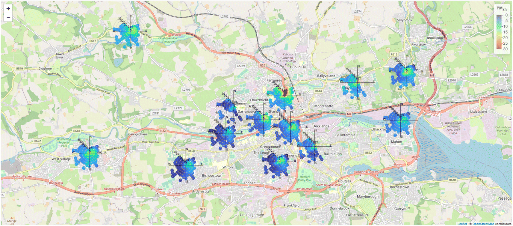
The AQS PM 2.5 network operated by Cork City Council is made up of 16 PurpleAir PA-II-SD units distributed across the city. The locations of the PurpleAir (PA) units are shown in Fig. 1. Each PA unit consists of two Plantower PMS5003 sensors to measure PM2.5 and PM10 mass concentrations (in μg m−3) based on light scattering. PA units and other systems based on the PMS5003 sensors are widely used for monitoring PM concentrations and, in general, their measurements are highly correlated with PM levels measured by gold-standard instrumentation.21,22 The measurement alternates between the two sensors every 5 seconds and the average for each sensor is obtained over a 120 second period. Data is uploaded to the PurpleAir online platform via a WiFi connection and the data is also recorded on an SD card. The PA devices contain a Bosch BME280 sensor for pressure, temperature, and humidity readings. Raw sensor data is available freely via the PurpleAir website (https://map.purpleair.com/). | ||
| Fig. 1 Map of Cork city with PA locations. | ||
2.2 Data sources and preparation
The same steps were applied to all data retrieved from the PA units in the sensor network to create a data set of hourly values between 01/01/2021 and 31/12/2021. The PA network dataset comprised a total of 228371 individual hourly measurements. Although these dates incorporated some periods of COVID-19 pandemic restrictions, such restrictions mostly affected NO2 concentrations and have not been found to have an unequivocal impact on PM levels in Ireland5
The correlation between the two internal sensors in each device was investigated. Both sensors were highly correlated (R2 > 0.98) and agreed closely with each other (Table S1†). These values were obtained using the two data channels with common timestamps after quality assurance steps were carried out. The excellent correlation between the two sensors in each device demonstrates that sharp changes in the high frequency data are linked to changes in atmospheric composition and do not arise from measurement noise.
2.3 Air quality sensor performance evaluation
A multiple linear regression (MLR) model was used to correct the hourly PA data. An MLR is used to assess the association between two or more independent variables and a single continuous dependant variable and can be expressed using the general equation:
| Ŷ = c0 + c1X1 + c2X2 +…cnXn | (1) |
The MLR model incorporated the known effects of relative humidity and temperature on PM measurement.26 Multiplicative terms were also included to capture the full relationship between PM and the meteorological variables. However, the coefficients of multiplicative terms were small and these terms were ignored in applying the calibration equation to the data. The full calibration equation is:
| Ŷ = −5.63 + 0.80(X) + 0.19(T) + 0.06(RH) − 0.00002(X × T) − 0.003(X × RH) − 0.0001(T × R) − 0.0002(X × RH × T) | (2) |
The PA and BAM measurements were well correlated (R2 = 0.9203) with a small offset (0.3 μg m−3). The PA measurements were consistently higher than the reference measurements (slope = 0.57), as has been found in previous studies with PA devices and other air quality sensors.27–29 After applying the correction, good agreement between the reference and PA measurements is observed, although the corrected PA values are somewhat lower than the reference data under high aerosol loading (Fig. S1 and S2†).
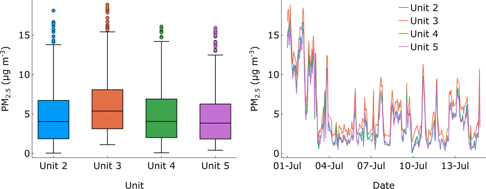 | ||
| Fig. 2 Box plots and time series for uncorrected data from Units 2, 3, 4, and 5 obtained during the inter-unit sensor comparison period. | ||
3 Results and discussion
3.1 Spatial and temporal variation in PM2.5 pollution
The calibrated network of PA units was used to analyse the spatial and temporal variations in PM2.5 across Cork city. The units were categorised by their location in the city (Table 1). Note that the devices located in the commuter towns are within the official city boundary.| Location type | Device label | Max diurnal PM2.5 (μg m−3) |
|---|---|---|
| North | ccc4 | 13.4 |
| ccc6 | 9.0 | |
| ccc14 | 18.9 | |
| South | ccc1 | 10.1 |
| ccc5 | 11.2 | |
| ccc9 | 14.1 | |
| East | ccc2 | 11.4 |
| ccc12 | 14.8 | |
| ccc13 | 14.5 | |
| West | mtu | 7.5 |
| ccc8 | 8.9 | |
| City centre | ucc | 11.3 |
| ccc3 | 9.1 | |
| ccc11 | 11.5 | |
| Commuter towns | ccc15 | 19.4 |
| ccc7 | 10.2 |
| Unit 2 | Unit 3 | Unit 4 | Unit 5 | Mean (μg m−3) | Max (μg m−3) | |
|---|---|---|---|---|---|---|
| Unit 2 | 5.05 | 18.11 | ||||
| Unit 3 | 0.989 | 6.37 | 18.87 | |||
| Unit 4 | 0.989 | 0.992 | 4.96 | 16.09 | ||
| Unit 5 | 0.989 | 0.988 | 0.991 | 4.75 | 15.93 |
The winter (01/10/2021–31/12/2021) diurnal profiles for PM2.5 (Fig. 3) show the expected pattern for locations in Ireland where residential solid-fuel burning emissions dominate. The air temperature in Ireland generally starts to drop in October so to capture the effect of the full heating season we take October as the beginning of winter. In contrast, the diurnal profiles for the summer months (01/06/2021–31/08/2021) shows lower levels of PM2.5 and minimal variation across the day (Fig. 4). Winter PM2.5 concentrations around noon are similar to those in summer. However, from about 15:00 on winter days, there is a sharp increase in PM2.5 as households start burning solid fuel for home heating.
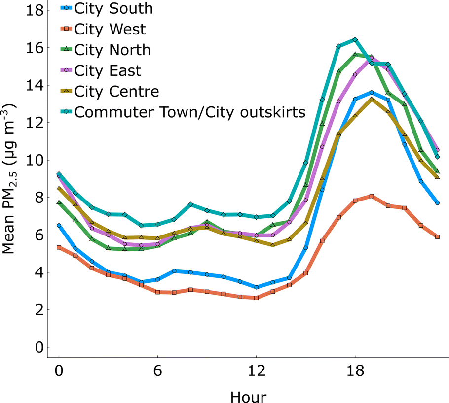 | ||
| Fig. 3 2021 Winter PM2.5 diurnal averages per location type. | ||
 | ||
| Fig. 4 2021 Summer PM2.5 diurnal averages per location type. | ||
Although the same diurnal pattern is observed across the city, marked differences are seen in the maximum PM2.5 levels in different regions of the city, indicating that residents in some parts of the city are exposed to appreciably higher PM concentrations than those in other areas. The devices categorised as city west showed diurnal profiles with peak PM2.5 concentrations about half of those in other areas. Surprisingly, the outlying commuter towns (Blarney and Ballincollig) experienced the highest daily average for PM2.5 concentrations, even above those of neighbourhoods within the contiguous built-up areas of Cork city. While the values of PM2.5 are indicative due to the nature of the sensors, the data provides clear evidence of the relative variation in PM2.5 concentrations between location types and seasons.
The comparison of overall average PM2.5 concentrations for the summer and winter periods is shown in Fig. 5. The commuter towns experienced the largest increase in PM levels from summer to winter. Based on the diurnal profiles, the large seasonal PM2.5 difference in these location types points towards a major impact from solid fuel burning.
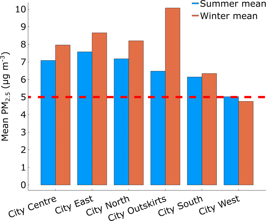 | ||
| Fig. 5 2021 PM2.5 averages over summer and winter periods per city district with WHO AQG annual mean (5 μg m−3) indicated. | ||
The diurnal profiles show the total hourly average PM2.5 levels in a location across a given period, however it is also important to consider the effect of pollution events which may not be apparent when looking at the average values. The maximum hourly average from the winter dataset was found for each location type. Table 3 compares these values to the maximum values seen in the diurnal profiles along with the mean value for the winter period. The commuter town locations showed a diurnal average peak around double that of the city west devices, while they had similar maximum hourly averages. This suggests that while a location type may experience lower PM levels on average relative to elsewhere in the city, there can still be significant exposure to high levels of PM2.5 during pollution events.
| North | South | East | West | Centre | Commuter towns | |
|---|---|---|---|---|---|---|
| Diurnal average maximum (μg m−3) | 15.6 | 13.6 | 15.5 | 8.1 | 13.3 | 16.4 |
| Hourly average maximum (μg m−3) | 84.2 | 99.8 | 57.6 | 49.2 | 73.2 | 56.7 |
| Mean (μg m−3) | 8.2 | 6.3 | 8.7 | 4.8 | 8.0 | 10.1 |
3.2 Identification and estimation of local emissions
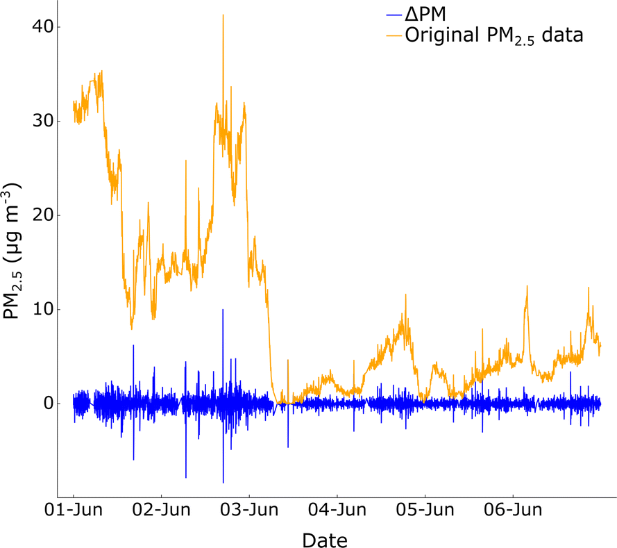
High frequency time series data from the network units exhibited intense, short-lived spikes in PM2.5 concentrations (Fig. 6). These spikes predominantly occurred on winter evenings. Across the network, both sensors A and B in the different PA units consistently showed the same behaviour with a high correlation coefficient between the two sensors, including during the spikes (Table S1†). We conclude therefore that the spikes are not measurement noise but indicate rapid variations in the PM concentrations measured by the different sensor units.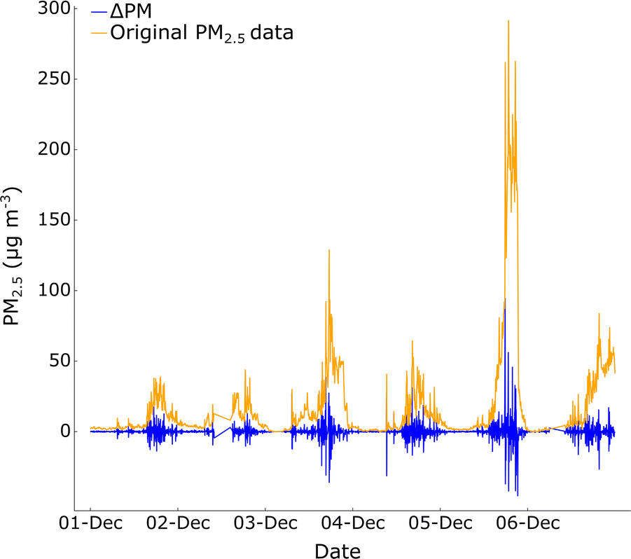 | ||
| Fig. 6 Example time series for unit ccc9 with ΔPM during the first week of December 2021. | ||
The high-frequency (2 minute interval) data was analysed to investigate the contribution of local area emissions of PM2.5 to the total PM2.5 burden across the city. Using uncorrected PM2.5 data obtained by the PurpleAir devices for June and December (to represent summer and winter and to ensure sufficient sensor data was available during analysis), the difference between two consecutive measurements (ΔPM) was calculated:
| ΔPMt = PMt − PMt−1 | (3) |
 | ||
| Fig. 7 Example time series for unit ccc9 with ΔPM during the first week of June 2021. | ||
Hourly standard deviations of ΔPM (σΔPM) were calculated to investigate the variability in PM concentrations at different times:
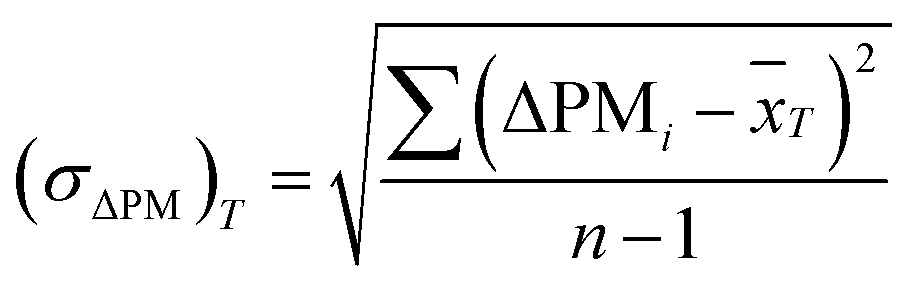 | (4) |
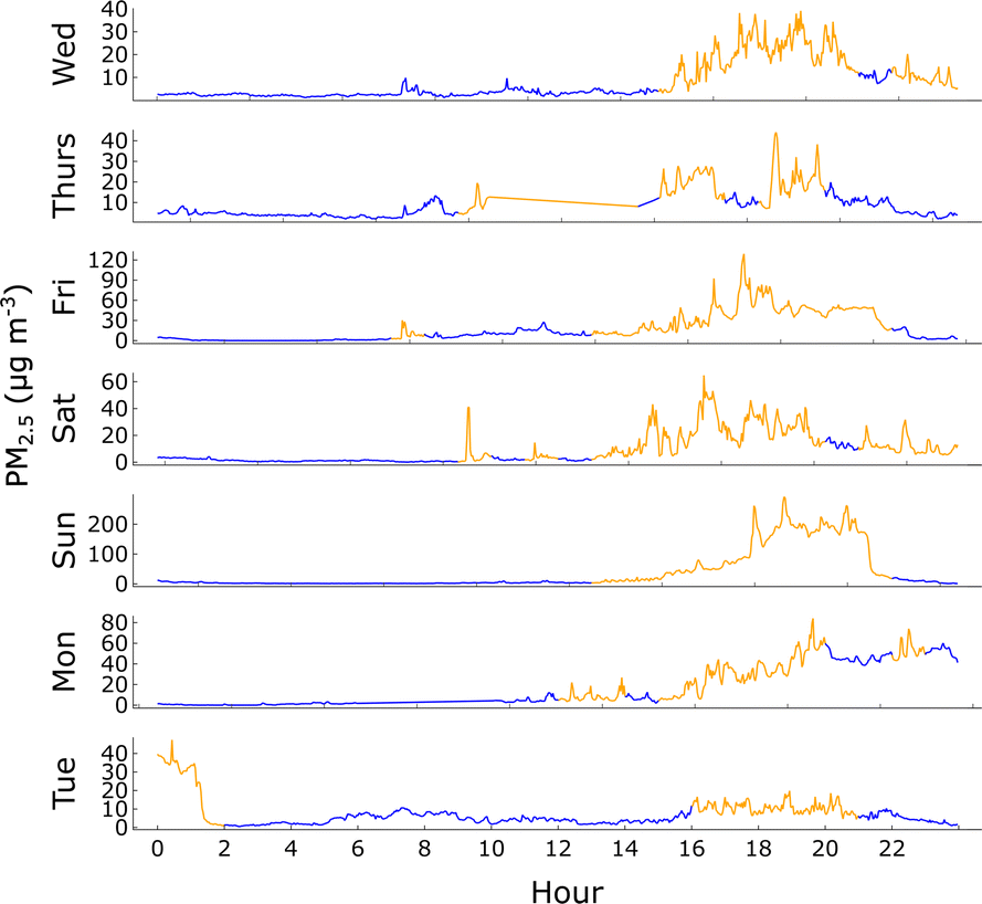
 is the mean of ΔPM over hour T, and n is the total number of ΔPM values in hour T. This approach was selected to identify periods of rapid fluctuations in measurements and to ensure that the selection process was not influenced by the background concentration or more gradual changes in PM levels over time. To identify periods of rapid fluctuations, periods where the hourly standard deviation was greater than 2 μg m−3 were highlighted, as shown on the unit ccc9 data in December (Fig. 8) and June (Fig. 9). In these figures, the data points in blue correspond to periods of low deviation from the hourly mean, and the periods in yellow correspond to the instances highlighted by the σΔPM filtering process where there is higher deviation from the hourly mean value, indicating rapid fluctuations in PM levels. The use of a standard deviation limit of 2 μg m−3 was based on a trial-and-error approach which used visual inspection to determine whether periods of rapid fluctuations in the data were appropriately captured. Limits of 1 and 3 μg m−3 were also assessed but were not as effective in discriminating periods of rapid PM fluctuations.
 | ||
| Fig. 8 σ ΔPM filter applied to unit ccc9 for the first week in December 2021. Blue data points correspond to periods of low σΔPM, yellow data points correspond to periods of high σΔPM. | ||
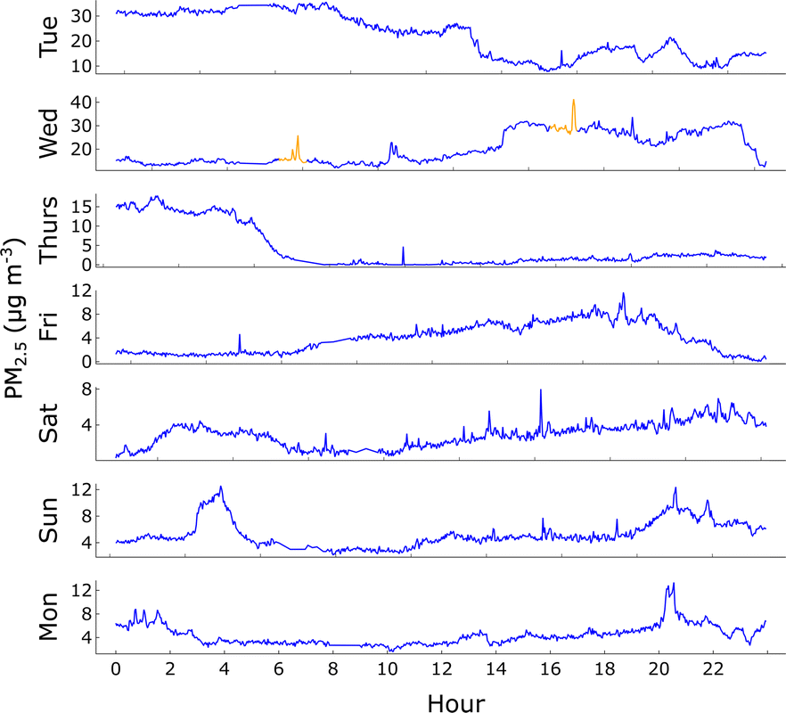 | ||
| Fig. 9 σ ΔPM filter applied to unit ccc9 for the first week in June 2021. Blue data points correspond to periods of low σΔPM, yellow data points correspond to periods of high σΔPM. | ||
Periods of large fluctuations in PM concentrations (where the data deviated appreciably from the hourly mean) were much more frequent in December than in June. These rapid fluctuations typically occurred at times when solid fuels are burnt for home heating. Large fluctuations in PM2.5 levels are sometimes also a feature of sites impacted by intermittent, high traffic emissions such as at busy traffic junctions. Traffic emissions are unlikely to be a major contributor to the Cork AQS network as the rapid fluctuations were a common characteristic across all PA units in the network, despite the fact that most PA units were not immediately adjacent to busy roads and intersections.
The average σΔPM across each daily hour for June and December was calculated. On average, hour 18 (6–7 pm) has the highest hourly standard deviation in December, with the lowest standard deviation seen in the early morning hours (despite relatively high PM levels). The winter month shows higher hourly standard deviation of ΔPM compared to the warmer summer month by a factor of 2.5 on average. The percentage of times with high hourly fluctuations was calculated (Table 4). PM2.5 concentrations in the various locations had markedly different profiles for the winter period, with the proportion of time with high fluctuation periods ranging from 8% to 55%.
| Device | Location type | Percent of time identified as having local influence | Percent of total PM2.5 observed during locally influenced periods | Percent of additional PM2.5 observed attributable to local emissions | |||
|---|---|---|---|---|---|---|---|
| June | December | June | December | June | December | ||
| % | % | % | % | % | % | ||
| ccc4 | North | 5 | — | 7 | — | 7 | — |
| ccc5 | South | 5 | 30 | 7 | 56 | 7 | 55 |
| ccc9 | South | 4 | 36 | 7 | 75 | 6 | 74 |
| ccc2 | East | 8 | 34 | 8 | 56 | 7 | 55 |
| ccc12 | East | 4 | 41 | 5 | 57 | 6 | 57 |
| ccc13 | East | 18 | 55 | 28 | 87 | 27 | 87 |
| mtu | West | 5 | 16 | 7 | 38 | 7 | 37 |
| ccc8 | West | 2 | 11 | 5 | 25 | 5 | 24 |
| ucc | City centre | 1 | 8 | 3 | 24 | 3 | 23 |
| ccc11 | City centre | 14 | 24 | 17 | 41 | 17 | 40 |
| ccc7 | Commuter town | 22 | 41 | 21 | 61 | 19 | 60 |
| ccc15 | Commuter town | — | 36 | — | 61 | — | 60 |
| Average | 8 | 30 | 10 | 53 | 10 | 52 | |
To estimate the difference in measured PM2.5 levels between periods of high frequency fluctuations and periods of more stable PM2.5 levels, the relative differences were assessed using integration of the concentration–time profile. The total area under the PM2.5 concentration–time profile (AT) represents 100% of the exposure. The total integrated area under the profile of all high fluctuation periods for a given device (AF) represents the PM2.5 exposure that was associated with high frequency periods and the fraction AF/AT represents the percentage of PM2.5 exposure experienced during high frequency periods. These values are reported for both June and December in Table 4. During December, the AF/AT values for each location show considerable variation, with estimated percentages ranging from 24 to 87%. This variation is less apparent in June, with consistently low values measured by most devices. These figures, when compared with the percentage of time that locations experienced high frequency variations in PM2.5 levels, suggest that on average, 53% of the PM2.5 was measured during 30% of the time across the network locations during December. In other words, for a resident population, over half of their PM2.5 exposure occurred during a third of the time, and based on the σΔPM analysis above it is argued that the PM2.5 emissions during those periods originated in the local area. One further estimate can be developed, which is the portion of PM2.5 that is specifically attributable to local emissions above the background levels during the periods identified by the high frequency filter used in this study. If the integrated area Af represents the area under the curve above a threshold defined as the background level, then Af/AT represents an estimate of the additional PM2.5 in the locality that is due to emissions in the vicinity of the sensor. The background level here is taken as the level interpolated between the start time and the end time of each high frequency period. Estimates of both AF/AT and Af/AT are included in Table 4. Interestingly, the two estimates are almost identical numerically, which suggests that without local emissions the PM2.5 levels would be considerably lower than what was measured in this study.
This observation suggests that when the ΔPM filter is applied across a network of PA sensors, it can be used to distinguish between areas which experience greater levels of highly local PM pollution from those that experience city-wide PM. The high hourly standard deviation of ΔPM indicates periods with short-lived pollution events in a specific area. Based on previous work, such intense pollution is associated with smoke plumes from nearby chimneys.6,10,30 Of course, changes in wind speed and direction may also affect the air pollution in an area. However sustained changes in air pollution are associated with transported air masses from different directions while rapid fluctuations are associated with local emissions. The method employed here allows discrimination between these pollution sources. Furthermore, the high temporal resolution of the PA sensor measurements shows that the rapid fluctuations in PM levels are a characteristic feature of wintertime air pollution in Ireland. Such short-lived plumes would be missed with a lower temporal resolution, such as with hourly data.
Our Af/AT estimate assumes that the baseline level is not significantly changed and follows the same rationale as the Lenschow, or incremental, approach and is subject to similar dependencies.31,32 In the incremental approach, the urban impact is taken as the sum of the following terms: the Lenschow urban increment, the city spread and the background deviation.33 In the approach presented here, local impact is confounded with the city spread, while the background is considered as the baseline level when local sources are non-dominant. Notably, our AF/AT estimate makes no such assumption, but supports the same conclusion.
Analysis of the spatial and temporal variations in PM2.5 across Cork City showed that the impact of local PM emissions varied from location to location, as shown by the differences in the diurnal averages across location types and in the winter and summer averages (Fig. 3 and 4). The results showed that the devices categorised as City West showed the lowest PM concentrations during winter, with the sensors in the commuter towns showing the highest diurnal peak of all locations (Table 3). However, all location types experienced high maxima (Table 3). This was in stark contrast to the average air quality being experienced for the overall period. The results show that while certain areas may experience lower daily average PM2.5 overall during winter, they can at times experience strong maximum peaks resulting from more severe pollution events over the winter season. The results from this analysis provide support for the emission classifications given in Section 3.2. The estimated local contributions varied considerably across the devices, with some locations experiencing over double the local estimated contributions of others. The difference between the winter and summer results in the emission classification correlates well with the spatial and temporal variation analysis. By looking at the average PM2.5 levels across the winter and summer months, it was shown that there are significant differences in PM2.5 levels between the two periods and between locations. This is also shown with the emission classification estimates. During the colder period in December, there were elevated levels of estimated local PM2.5 contributions, with some locations experiencing higher levels than others. In particular, the devices located in smaller suburban areas further from the city centre showed significant local PM2.5 contribution estimates, comparable to or even higher than the more urban counterparts. For example, the device ccc15, located in Ballincollig, a commuter town approximately 9 km outside of the city centre, experienced one of the highest local PM2.5 contribution estimates during the winter period, which relates to the high winter averages seen in the spatial and temporal analysis. During the month of June, the estimated contribution of local PM2.5 for all locations remained low and stable. This relates to the similar summer averages shown across the location types previously.
3.3 Meteorological factors
It is a common observation that an important factor determining PM2.5 levels in a locality is the weather. Emissions generally follow economic cycles and tend to exhibit regular patterns, whereas the weather is highly variable. So the weather affects the PM2.5 levels by (i) influencing emissions, such as causing increased home heating and energy use during cold periods and (ii) dispersion of emissions, such as effective transport of pollution by wind, with generally better mixing and dispersion at higher wind speeds. The weather is not generally responsible for generating PM2.5 emissions, although PM10 levels can increase at higher wind speeds due to increased resuspension by wind.The argument that is developed here is that during periods of less effective atmospheric mixing, i.e. at low wind speeds, the emissions are not dispersed effectively, and they build up in the local area where they are emitted. The prevailing wind direction in Cork city is from the South–West. However, as shown in the wind rose in Fig. S3,† during the period covered in this study, this pattern was not as evident and the weather was less dominated by the prevailing wind direction than is normally the case.
Fig. 10 shows polar plots for each device location indicating the wind direction and wind speed associated with higher PM2.5 concentrations in each location. For some locations situated on the periphery of the city, such as the devices labelled mtu and ccc8, located at the western edge of the city, the higher PM2.5 levels are clearly associated low wind speeds from the easterly direction. For the most part, however, there is no consistent directionality to the PM2.5 concentrations. Higher PM2.5 is always associated with low wind speeds. These observations are again consistent with the suggestion that PM2.5 levels are dominated by nearby emissions.
 | ||
| Fig. 10 Polar plots showing associations between wind speed and direction, and local PM2.5 levels at the locations monitored in the sensor network. | ||
The meteorological data obtained from Met Éireann reflect the weather on a synoptic scale while the meteorological field across the city will also be influenced by local factors, street canyons and local topography. It therefore cannot be assumed that the wind direction measured at the airport (approximately 4–11 km from individual devices) is identical for all devices in the network. Nevertheless, the regional scale wind direction will dominate the general meteorological field across the city and it can be reasonably supposed that transport of ambient PM2.5 would be observable as a concentration gradient across the area if such transport was a significant factor in observed PM2.5 levels. Wind speeds measured at the airport, which is situated in an elevated location above the city, generally exceed those experienced in the city. In other words, while the wind direction measured at the airport may have deviated from the wind direction at a given device, the fact that the polar plots imply no particular directionality suggests that wind direction is not an important factor. Moreover, the fact that higher PM2.5 levels are associated with low wind speeds in general supports the hypothesis of very local origin.
3.4 Comparison with source apportionment studies
The measurements and estimates reported in Table 4, particularly for December, suggest that measured PM2.5 levels could mainly be attributed to residential solid fuel burning. A comparison with previous source apportionment studies in Cork and other places in Ireland, may therefore be instructive. Detailed source apportionment studies have been previously carried out in the Port of Cork, but they are separated from this study by over a decade. Using chemical markers associated with the combustion of peat, coal and wood, the estimated contribution of local solid fuel burning to PM2.5 concentrations measured at the Port of Cork in August 2008 was 5%.30 Using a different approach, Kourtchev et al.,6 obtained a value of 6% for the solid fuel burning contribution during the same period. These values are in line with the local PM2.5 contribution estimates reported for many locations during June (Table 4), including ccc2, which is the PA unit closest to the Port of Cork measurement site. Kourtchev et al.,6 also obtained a value of 28% for the solid fuel burning contribution to PM2.5 measured during February 2009, while a more comprehensive source apportionment method was used by Dall'Osto et al.34 to deliver an estimate of 46–50% for the same period. The results of this latter study are more consistent with the local PM2.5 contribution estimates obtained for December 2021 in this work, Table 4. A more recent study employing detailed in situ chemical characterisation of ambient wintertime PM2.5 and source apportionment modelling has been carried out at multiple diverse locations in Ireland, including the capital city, Dublin, a small midland town (Birr) and costal locations (Carnsore Point and Mace Head). Average estimates of local solid fuel contributions were 50%, 25%, 48% and 39%, for Dublin, Carnsore Point, Birr, and Mace Head, respectively.8 The results obtained for the urban areas of Dublin and Birr are in line with local PM2.5 contribution estimates obtained for December 2021 in this work, Table 4.While other studies have utilised air quality sensors in similar ways to estimate source contributions, these are based on measurements in different environments where the resulting estimates would not be comparable to the specific results presented here.35–37 They do, however, showcase the usefulness and feasibility of using these kinds of devices in new and meaningful ways to attain more in-depth information about an area's air quality without using traditional and more costly facilities and instrumentation.
4 Conclusions
The PA sensor network in Cork city has provided information on the spatial and temporal variations in PM2.5 across the urban area that were previously unachievable with traditional air quality monitoring methods. The accuracy of the measurements was improved by calibrating the sensor network through a co-location study with a reference monitor. While the PA data is considered indicative and not of regulatory monitoring standard, this study showcases the opportunities available with an AQS network. In particular, a carefully planned and implemented AQS network delivers complementary information to that from a regulatory grade air quality monitoring network. This includes expanding monitoring across cities where regulatory monitoring is already in place. Such AQS networks can provide valuable information on local air quality in a context where regulatory monitoring network is unaffordable, such as in developing country cities and in smaller towns in wealthy nations.This study also shows it is possible to distinguish between local and background/other emissions using a PM sensor network. Such information is vital for developing targeted and effective interventions to improve urban air quality. We applied a novel method using high frequency data to highlight time periods where the PM measured by the AQS is assumed to be dominated by an intense local pollution source as opposed to a background/other source in the city. Significant differences were found between the different locations, in particular between devices west of Cork city and in the other areas of the city. The western locations had higher PM2.5 levels associated with easterly winds of low wind speed and were among the lowest in terms of percent of time with high fluctuations and percent of PM2.5 measured during these periods. However, the majority of devices showed higher PM2.5 levels with low wind speeds, but no consistent directionality, suggesting that local emission sources dominate the PM2.5 levels.
The considerable differences in estimated local contributions highlights the importance of measuring in multiple locations within an urban area. Surprisingly, the surrounding commuter towns were found to have local PM contribution estimates that were on par with or above those of other location types. This shows that less populated locations and small towns can experience higher PM2.5 levels than areas closer to the city centre. Nevertheless, all location types experienced high daily maxima, indicating that while daily average values may differ appreciably at locations across the city owing to higher instances of residential solid fuel burning or favourable meteorological conditions, all areas experience pollution episodes with high PM2.5 concentrations.
Author Contributions
KR provided the data for the project. RB and SH conducted the formal data analysis. RB wrote the manuscript with contributions from SH, JCW, and DSV.Conflicts of interest
There are no conflicts to declare.Acknowledgements
The research carried out was supported by the EPA and DECC and the EU LIFE Programme through the project LIFE Emerald – LIFE19 GIE/IE/001101. The authors also acknowledge Cork City Council for developing and maintaining the air quality sensor network. In particular, Rob Bateman, a technician seconded to Cork City Council who assisted with the physical deployment of the air quality units across the city.References
- N. T. Waidyatillake, P. T. Campbell, D. Vicendese, S. C. Dharmage, A. Curto and M. Stevenson, Particulate matter and premature mortality: A Bayesian meta-analysis, Int J Environ Res Public Health, 2021, 18, 7655, DOI:10.3390/ijerph18147655.
- K.-H. Kim, E. Kabir and S. Kabir, A review on the human health impact of airborne particulate matter Human health Particle size, Environ Int, 2015, 74, 136–143, DOI:10.1016/j.envint.2014.10.005.
- S. Sang, C. Chu, T. Zhang, H. Chen and X. Yang, The global burden of disease attributable to ambient fine particulate matter in 204 countries and territories, 1990–2019: A systematic analysis of the Global Burden of Disease Study 2019, Ecotoxicol Environ Saf, 2022, 238, 113588, DOI:10.1016/j.ecoenv.2022.113588.
- Health Effects Institute, State of Global Air 2020, Boston, MA, 2020, https://www.stateofglobalair.org/ Search PubMed.
- Environmental Protection Agency (EPA), Air Quality in Ireland 2020, 2020, https://www.epa.ie/publications/monitoring–assessment/air/air-quality-in-ireland-2020.php Search PubMed.
- I. Kourtchev, S. Hellebust, J. M. Bell, I. P. O'Connor, R. M. Healy, A. Allanic, D. Healy, J. C. Wenger and J. R. Sodeau, The use of polar organic compounds to estimate the contribution of domestic solid fuel combustion and biogenic sources to ambient levels of organic carbon and PM2.5 in Cork Harbour, Ireland, Science of The Total Environment, 2011, 409, 2143–2155, DOI:10.1016/scitotenv.2011.02.027.
- C. Lin, R. J. Huang, D. Ceburnis, P. Buckley, J. Preissler, J. Wenger, M. Rinaldi, M. C. Facchini, C. O'Dowd and J. Ovadnevaite, Extreme air pollution from residential solid fuel burning, Nat Sustain, 2018, 1, 512–517, DOI:10.1038/s41893-018-0125-x.
- C. Lin, D. Ceburnis, R. J. Huang, W. Xu, T. Spohn, D. Martin, P. Buckley, J. Wenger, S. Hellebust, M. Rinaldi, M. Cristina Facchini, C. O'Dowd and J. Ovadnevaite, Wintertime aerosol dominated by solid-fuel-burning emissions across Ireland: Insight into the spatial and chemical variation in submicron aerosol, Atmos Chem Phys, 2019, 19, 14091–14106, DOI:10.5194/acp-19-14091-2019.
- J. Wenger, J. Arndt, P. Buckley, S. Hellebust, E. Mcgillicuddy, I. O'Connor, J. Sodeau and E. Wilson, Source Apportionment of Particulate Matter in Urban and Rural Residential Areas of Ireland (SAPPHIRE), https://www.epa.ie/publications/research/environment–health/Research_Report_318.pdf Search PubMed.
- M. Dall'Osto, J. Ovadnevaite, D. Ceburnis, D. Martin, R. M. Healy, I. P. O'Connor, I. Kourtchev, J. R. Sodeau, J. C. Wenger and C. O'Dowd, Characterization of urban aerosol in Cork city (Ireland) using aerosol mass spectrometry, Atmos. Chem. Phys, 2013, 13, 4997–5015, DOI:10.5194/acp-13-4997-2018.
- C. Lin, D. Ceburnis, S. Hellebust, P. Buckley, J. Wenger, F. Canonaco, A. S. H. Prévôt, R. J. Huang, C. O'Dowd and J. Ovadnevaite, Characterization of Primary Organic Aerosol from Domestic Wood, Peat, and Coal Burning in Ireland, Environ Sci Technol, 2017, 51, 10624–10632, DOI:10.1021/acs.est.7b01926.
- J. Eakins, B. Power, N. Dunphy and G. Sirr, Residential Solid Fuel Use in Ireland and the Transition Away from Solid Fuels, 2022, https://www.epa.ie/publications/research/air/Research_Report_407.pdf Search PubMed.
- Environmental Protection Agency (EPA), Air Quality in Ireland 2021, https://www.epa.ie/publications/monitoring–assessment/air/air-quality-in-ireland-2021 Search PubMed.
- D. Bousiotis, A. Singh, M. Haugen, D. C. S. Beddows, S. Diez, K. L. Murphy, P. M. Edwards, A. Boies, R. M. Harrison and F. D. Pope, Assessing the sources of particles at an urban background site using both regulatory instruments and low-cost sensors – a comparative study, Atmos Meas Tech, 2021, 14, 4139–4155, DOI:10.5194/amt-14-4139-2021.
- K. Brzozowski, A. Ryguła and A. Maczyński, The use of low-cost sensors for air quality analysis in road intersections, Transp Res D Transp Environ, 2019, 77, 198–211, DOI:10.1016/j.trd.2019.10.019.
- N. Castell, F. R. Dauge, P. Schneider, M. Vogt, U. Lerner, B. Fishbain, D. Broday and A. Bartonova, Can commercial low-cost sensor platforms contribute to air quality monitoring and exposure estimates?, Environ Int, 2017, 99, 293–302, DOI:10.1016/j.envint.2016.12.007.
- G. Kosmopoulos, V. Salamalikis, S. N. Pandis, P. Yannopoulos, A. A. Bloutsos and A. Kazantzidis, Low-cost sensors for measuring airborne particulate matter: Field evaluation and calibration at a South-Eastern European site, Science of the Total Environment, 2020, 748, 141396, DOI:10.1016/j.scitotenv.2020.141396.
- B. Alfano, L. Barretta, A. del Giudice, S. de Vito, G. di Francia, E. Esposito, F. Formisano, E. Massera, M. L. Miglietta and T. Polichetti, A Review of Low-Cost Particulate Matter Sensors from the Developers' Perspectives, Sensors, 2020, 20, 6819, DOI:10.3390/s20236819.
- S. de Vito, E. Esposito, N. Castell, P. Schneider and A. Bartonova, On the robustness of field calibration for smart air quality monitors, Sens Actuators B Chem, 2020, 310, 127869, DOI:10.1016/j.snb.2020.127869.
- Cork City Council and University College Cork, Cork City Council Air Quality Dashboard, https://www.corkairquality.ie/ Search PubMed.
- K. Ardon-Dryer, Y. Dryer, J. N. Williams and N. Moghimi, Measurements of PM2.5 with PurpleAir under atmospheric conditions, Atmos Meas Tech, 2020, 13, 5441–5458, DOI:10.5194/amt-13-5441-2020.
- T. Sayahi, A. Butterfield and K. E. Kelly, Long-term field evaluation of the Plantower PMS low-cost particulate matter sensors, Environ Pollut, 2019, 245, 932–940, DOI:10.1016/j.envpol.2018.11.065.
- J. Bezanson, A. Edelman, S. Karpinski and V. B. Shah, Julia: A fresh approach to numerical computing, SIAM Rev., 2017, 59, 65–98, DOI:10.48550/arXiv.1411.1607.
- D. C. Carslaw and K. Ropkins, Openair — An R package for air quality data analysis, Environmental Modelling & Software, 2012, 27–28, 52–61 Search PubMed.
- PurpleAir, PA-II SD Specs, https://www2.purpleair.com/collections/air-quality-sensors/products/purpleair-pa-ii-sd, (accessed 12 May 2022) Search PubMed.
- C. Malings, R. Tanzer, A. Hauryliuk, P. K. Saha, A. L. Robinson, A. A. Presto and R. Subramanian, Fine particle mass monitoring with low-cost sensors: Corrections and long-term performance evaluation, Aerosol Science and Technology, 2020, 54, 160–174, DOI:10.1080/02786826.2019.1623863.
- N. Karaoghlanian, B. Noureddine, N. Saliba, A. Shihadeh and I. Lakkis, Low cost air quality sensors “PurpleAir” calibration and inter-calibration dataset in the context of Beirut, Data Brief, 2022, 41, 108008, DOI:10.1016/j.dib.2022.108008.
- A. Datta, A. Saha, M. L. Zamora, C. Buehler, L. Hao, F. Xiong, D. R. Gentner and K. Koehler, Statistical field calibration of a low-cost PM2.5 monitoring network in Baltimore, Atmos Environ, 2020, 242, 117761, DOI:10.1016/j.atmosenv.2020.117761.
- P. Gupta, P. Doraiswamy, J. Reddy, P. Balyan, S. Dey, R. Chartier, A. Khan, K. Riter, B. Feenstra, R. C. Levy, N. Nguyen, M. Tran, O. Pikelnaya, K. Selvaraj, T. Ganguly and K. Ganesan, Low-Cost Air Quality Sensor Evaluation and Calibration in Contrasting Aerosol Environments, Atmos Meas Tech DOI:10.5194/amt-2022-140.
- R. M. Healy, S. Hellebust, I. Kourtchev, A. Allanic, I. P. O'Connor, J. M. Bell, D. A. Healy, J. R. Sodeau and J. C. Wenger, Source apportionment of PM2.5 in Cork Harbour, Ireland using a combination of single particle mass spectrometry and quantitative semi-continuous measurements, Atmos Chem Phys, 2010, 10, 9593–9613 CrossRef CAS.
- P. Lenschow, H. J. Abraham, K. Kutzner, M. Lutz, J. D. Preuß and W. Reichenbächer, Some ideas about the sources of PM10, Atmos Environ, 2001, 35, S23–S33 CrossRef CAS.
- J. Pey, X. Querol and A. Alastuey, Discriminating the regional and urban contributions in the North-Western Mediterranean: PM levels and composition, Atmos Environ, 2010, 44, 1587–1596 CrossRef CAS.
- P. Thunis, On the validity of the incremental approach to estimate the impact of cities on air quality, Atmos Environ, 2018, 173, 210–222 CrossRef CAS.
- M. Dall'Osto, S. Hellebust, R. M. Healy, I. P. Connor, I. Kourtchev, J. R. Sodeau, J. Ovadnevaite, D. Ceburnis, C. D. O'Dowd and J. C. Wenger, Apportionment of urban aerosol sources in Cork (Ireland) by synergistic measurement techniques, Science of The Total Environment, 2014, 493, 197–208 CrossRef PubMed.
- S. C. C. Lung, W. C. V. Wang, T. Y. J. Wen, C. H. Liu and S. C. Hu, A versatile low-cost sensing device for assessing PM2.5 spatiotemporal variation and quantifying source contribution, Science of The Total Environment, 2020, 716, 137145 CrossRef CAS PubMed.
- C. G. Hodoli, F. Coulon and M. I. Mead, Source identification with high-temporal resolution data from low-cost sensors using bivariate polar plots in urban areas of Ghana, Environmental Pollution, 2023, 317, 120448 CrossRef CAS PubMed.
- I. Heimann, V. B. Bright, M. W. McLeod, M. I. Mead, O. A. M. Popoola, G. B. Stewart and R. L. Jones, Source attribution of air pollution by spatial scale separation using high spatial density networks of low cost air quality sensors, Atmos Environ, 2015, 113, 10–19 CrossRef CAS.
Footnote |
| † Electronic supplementary information (ESI) available. See DOI: https://doi.org/10.1039/d2ea00177b |
| This journal is © The Royal Society of Chemistry 2023 |