Evaluation of low-cost gas sensors to quantify intra-urban variability of atmospheric pollutants

Abstract

Low-cost air quality monitoring units were tested within the context of the European research project TRAFAIR. This study aims to quantify the intra-urban variability of atmospheric pollutants by means of a low-cost sensor network, which was deployed across the urban area of Modena, in the Po Valley (Italy) for the assessment of air quality in the city. Each sensor unit featured a set of electrochemical cells responding to NO, NO₂ and O₃ delivering a current/voltage proportional to the mixing ratio of the target atmospheric pollutant. Each unit was calibrated using field colocation next to an urban regulatory air quality monitoring station in the city. A machine learning Random Forest algorithm was used as a calibration model and different configurations of the model were applied. The results from these configurations were compared in terms of their prediction performance and consistency of the explanatory variable role within the model. A significant variability in all pollutants across town was revealed by the units, highlighting areas impacted by local sources.

---

Environmental significance

The development of low-cost electrochemical sensors has opened up new possibilities for monitoring air quality. Low-cost sensors have the ability to provide measurements of air pollutants close to real-time at a spatial resolution corresponding to the neighborhood scale if they are installed in dense urban networks. They can provide information about the impact of local pollution sources on various temporal and spatial scales, which the typically dispersed regulatory monitoring networks would not be able to. Although regulatory air quality monitoring networks provide valuable information about long-term air quality trends, other measurements and models must be added to the data to get spatially more precise air pollution statistics. Given that air pollution concentrations can differ significantly over short distances, this additional information is relevant. As a result, new research has been conducted in an effort to collect geographically and temporally dense information on air pollution by collecting continuous measurements from a low-cost sensor network. Mobile measurements with low-cost sensors were used to map air pollution in the city of Modena, Northern Italy over various seasons and times of the day.

1 Introduction

There is a growing need for a significantly more localized air pollution measurement in urban areas to address large spatial variability in air quality within complex zones (e.g. cities), to meet citizen expectations and to improve epidemiological and exposure studies.^1–3 However the infrastructural and operational costs of a regulatory Air Quality Monitoring station (AQM) limit the density increase in the existing regulatory monitoring networks.^1,4 Among possible solutions to this challenge are Land Use Regression Models,⁵ microscale dispersion modelling,⁶ and lower cost sensing technologies for atmospheric compounds.³ All solutions require comparison and calibration using standardized equipment (i.e. a regulatory monitoring station). However, using these solutions could reduce the number of AQMs in an urban area, while increasing the spatial coverage at a similar cost.

There is steadily rising interest in the use of lower cost technologies (here after named “low-cost sensors” (LCSs) for the sake of simplicity) by the scientific community, environmental agencies, local administrations and citizens. These sensors employ several established measurement principles: light scattering (for aerosols), non-dispersive infrared, photo-ionization detection, metal-oxide resistance and amperometric cells.^1,7,8 Amperometric cells recently received a significant improvement in design, leading to promising applications in atmospheric pollution, granted by an increased sensitivity to relevant compounds in air quality studies (e.g. NO, NO₂, and O₃).^8,9 Still these improved LCSs showed problems of stability, cross-sensitivity, calibration, low reproducibility, and low repeatability, requiring further testing and research.¹⁰ Among these issues, calibration is a process that can lead to improved results without the need for changes to the physical or chemical working principles of the sensor.¹¹ Calibration is also one of the major limiting factors for a broad and successful use of these devices: ideally a calibration should include a full description of the sensor physical or chemical working principles along with its response to all environmental conditions. Such an ideal calibration cannot be achieved given the current technology and understanding, requiring alternative approaches. Several calibration approaches for sensors were tested by the scientific community: laboratory validation under controlled conditions,¹² periodical field co-location next to a calibrated reference instrument,^2,13–15 and co-location followed by sensor to sensor calibration or remote calibration.¹⁶

Several previous studies investigated more specifically the effect on amperometric cells by a sensor relocation following a co-location period: Hagan et al.¹⁷ tested a short-term (a few days) calibration and relocation of SO₂ sensors, obtaining results fit for the purpose (i.e. volcanic plume detection); Bigi et al.¹⁴ employed a long term (4 months) calibration period to obtain an accuracy in relocation of ca. 20 ppb for hourly NO₂; Vikram et al.¹⁸ employed multi-site long term co-location calibration using machine learning algorithms to improve transferability, resulting in a median Mean Absolute Error (MAE) ca. 8 ppb for NO₂. Gordon Casey & Hannigan¹⁹ found that during relocation, when two AQM stations are too distant (over 40 km), an additional bias was introduced. Mailings et al.¹⁵ focused on the generalizability of a calibration model built upon a group of sensors to be applied on single third sensors, showing the influence by the regression algorithm and by the (calibration) sensor grouping. A similar approach and consistent findings were shown by Smith et al.²⁰ Moreover, meteorology is one of the drivers limiting the generalizability of a calibration model and this was addressed by Wei et al.²¹ by building a laboratory calibration model binned according to atmospheric temperature, improving the validation over long term (i.e. 4 months) and high model inner coherence (R² > 0.91) compared to commonly applied approaches. Most of these studies discussed this temporal/spatial co-location approach highlighting how the limited and site-specific range of environmental conditions observed during the calibration period raised issues about the generalizability of the derived calibration model, potentially leading to impaired results. More specifically Zimmerman et al.¹³ showed the key role played by the value range in the drivers which generated sensor response during colocation and how this affects the calibration performance. Recent studies (De Vito et al.²²) formally described this loss in performance and also provided a quantitative framework by investigating the change in the joint probability distribution of the variables causing a sensor response between the calibration and the deployment periods. Several of these studies, and others as well, showed and quantified also the impact on the final performance by using a regression algorithm model. Several of these authors^14,15,23,24 suggested machine learning algorithms, including Random Forest (RF):²⁵ RF relies on a training dataset to build a set of decision trees which are then used to provide model predictions. An inherent limitation of RF is the inability to extrapolate beyond its calibration space, thereby increasing the importance of the width of the training dataset and of its representation of the values that the model will be using in prediction.

Application studies of low cost sensor networks are growing: recently Peters et al.²⁶ as a part of the Breathe London pilot project used 100 stationary electrochemical NO₂ low cost sensors (LCSs) placed across Greater London for two years to assess sensor performance by collocating with reference instruments, calculating an average uncertainty of 35% in the calibrated LCSs, and identifying sporadic, multi-week periods of worse performance and significant bias over the summer. Zaidan et al.²⁷ used a dense network of air quality sensors in Nanjing, China along with methods for sensor validation and data interpretation to solve problems encountered during the implementation of a large-scale sensor network in a city. Kuula et al.²⁸ gave a well-informed perspective on specific aspects of the air quality directive which included air quality sensors as a component of a hierarchical observation network that would benefit from a re-evaluation. The information provided by such pilot studies is expected to be crucial in advancing studies on atmospheric chemistry, emission assessment and epidemiology, as recently pointed out by a recent perspective study (Sokhi et al.²⁹) describing current and future challenges and opportunities in atmospheric science. Most relevant to urban areas, LCS networks provide the capability to go beyond the standard paradigm, where atmospheric levels are observed at only a small number of representative locations with high accuracy, and are subsequently extrapolated to unmonitored areas by modelling.

In this work an urban wide low cost sensor (LCS) network was set up and ran for about 1.5 years in the urban site of Modena, in the Po valley, i.e. one of the largest European air pollution hotspots, which is an area with air quality levels exceeding EU regulations. 12 LCS units, featuring NO, NO₂ and O₃ sensors, were periodically calibrated (using a RF model) and rotated across 10 different locations in the town to provide reliable spatial and temporal intra-urban variability for these compounds.

2 Methods

The pilot study is based on the city of Modena in the Emilia-Romagna region of northern Italy. Modena (185 000 inhabitants) has a continental climate, with warm humid summers (a daily mean temperature of 25 °C), and dry cold winters (a daily mean temperature of 3 °C). Modena has rainfall mainly during Autumn and Spring seasons, with an annual climatological precipitation of ca. 800 mm.

Modena is regarded as one of the most polluted Italian cities. Vehicular traffic contributes significantly to air pollution. The city has a car density of 858 vehicles km⁻², higher than the Italian average of 764 vehicles km⁻² and, according to the latest local bottom-up inventory, referring to 2019 (ARPAE, 2022 (ref. 30)), vehicular traffic and domestic heating are responsible for 78% and 12% respectively of all NO_x emissions of the municipality.

2.1 Low-cost gas sensors

The air quality commercial units used in the study are the AirCube (Decentlab GmbH, Duebendorf, Switzerland). The units hosted four amperometric cells (ACs) by Alphasense as sensing elements to detect NO, NO₂, O₃ + NO₂ and CO, namely NO-B4, NO₂-B43F, O_x-B431 and CO-B4. The Alphasense cells feature two operational electrodes,⁸ a working electrode (WE) and an auxiliary electrode (AUX). The following notations are used throughout: the subscript _WE indicates the working electrode and the subscript _AUX indicates the difference between working and auxiliary electrodes, both are for the corresponding gas amperometric cell (e.g. NO_WE indicates the voltage from the working electrode for the NO-B4 cell).

The AirCube includes an air temperature (T) and relative humidity (RH) meteorological sensor (Sensirion STH21, Sensirion AG, Stäfa, Switzerland). The AirCube has an IP65 rated waterproof enclosure: this contains the electronics, the battery, the sensors and a hollow PTFE block with extensions for inlet and outlet. A small fan is installed inside the hollow PTFE block (also the meteorological sensor is installed inside) to draw the sample air. The external membrane of each amperometric cell faces the inner volume of this ventilated block. Each sampling cycle is as follows:

(1) Sensor measurements for 10 seconds.

(2) Air replacement using the small fan installed in the inlet.

(3) A waiting period of 40 seconds to allow the air to diffuse and equilibrate with the sensor cells (no air movement inside the PRFE block).

(4) New cycle starts.

The unit types collect voltage reading from the working and auxiliary electrodes of each cell, along with RH, T and battery voltage readings. These readings were transmitted to a central database using a dedicated LoRaWAN network.

12 sensor units were used in the current study. These units were used to monitor air quality at 10 locations within the urban area. These locations (see Table 1) were classified according to the main pollution conditions within the town as follows: urban traffic for sites at the kerbside of busy roads; urban residential for sites in residential areas with local traffic; urban background for sites in urban parks (PFR) or in the pedestrian area of the grounds of the main city hospital (PCU, PCM); urban low emission zone (LEZ) for the pedestrian area of the UNESCO heritage site within the LEZ of the town centre. The two sites at the main city hospital were active during different periods: PCM, from October 2019 to May 2020 and PCU since September 2020. PCM was discontinued due to the construction of a new building for hosting SARS-CoV-2 patients during the corresponding pandemics. Due to large similarity between PCM and PCU pollution conditions, they were considered as a single location and the observations were merged and analysed together.

Table 1 Monitoring location forming the low cost sensor network

Monitoring location	Acronym	Latitude	Longitude	Classification
a Sites GIA and PFR also hosted the regulatory AQM. b Active until May 2020. c Active since September 2020.
Via Giardini^a	GIA	44.6360°	10.9047°	Urban traffic
Parco Ferrari^a	PFR	44.6506°	10.9063°	Urban background
Via Alessandro volta	ALV	44.6450°	10.9135°	Urban residential
Via Pavia	PAV	44.6241°	10.9308°	Urban traffic
Piazza Manzoni	PMN	44.6344°	10.9293°	Urban traffic
Piazza Grande	PGR	44.6462°	10.9261°	Urban low emission zone
Policlinico^b	PCM	44.6350°	10.9437°	Urban background
Policlinico^c	PCU	44.6348°	10.9436°	Urban background
Via Villa d'Oro	VDO	44.6581°	10.9458°	Urban residential
MASA	MAS	44.6574°	10.9299°	Urban traffic
Ring Road	TNE	44.6296°	10.9532°	Urban traffic

---

The field campaign started in August 2019 and in the present work data up to April 2021 are considered.

Due to the periodic field calibration of each sensor by co-location at the AQM, not all locations were operational at the same time. In addition, a PCU and TNE were included at a later stage, while other sites have data gaps due to different malfunctions, maintenance, and calibrations. Fig. 1 shows the operational time for each location.

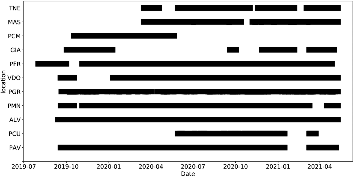Fig. 1 Operational low-cost sensor locations in Modena during 2019–2021.

2.2 Reference air quality stations

In the urban area of Modena there are two regulatory AQMs located at GIA and PCF representing urban traffic and urban background conditions respectively and hereafter referred to as MO_VG and MO_PF respectively. MO_VG is facing a 4 lane road near a busy junction and MO_PF is within the largest urban park. NO and NO_x measurements at 1 minute time resolution from both AQMs were provided by the local environmental agency (ARPAE Modena) in personal correspondence. Fig. 2 represents the map of the study area showing the city of Modena, the position of the low cost sensors (coloured circles), the AQMs (yellow stars) and the LoRaWAN gateways (green stars).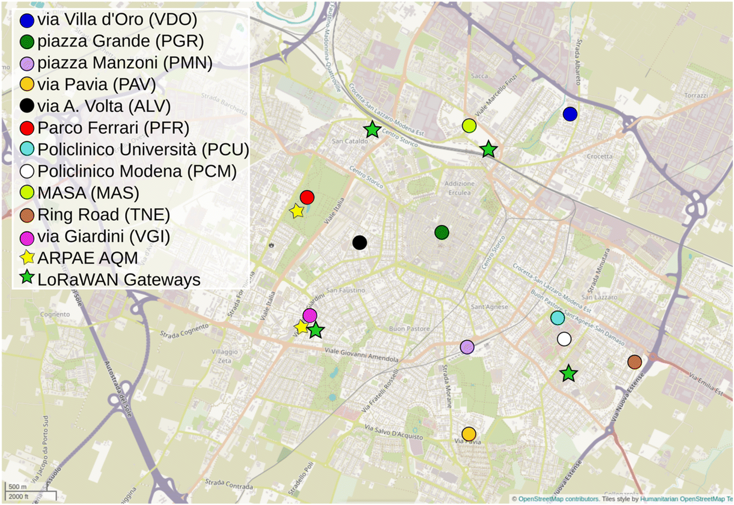

Fig. 2 Map of the AQ sensors, reference stations and LoRaWAN networks in Modena.

The local environmental agency³¹ reported in 2018 a yearly mean for NO₂ of 40 μg m⁻³ at MO_VG and a NO annual mean of 26 μg m⁻³ and 17 μg m⁻³ at MO_VG and MO_PF respectively. For the same period an annual average in NO₂ and O₃ of 27 μg m⁻³ and 45 μg m⁻³ respectively was observed at MO_PF. The same agency reported CO levels at the AQM consistently around the level of quantification of the CO regulatory monitor, which was eventually discontinued during the study period, preventing a calibration of the CO cell. Therefore, the analysis presented focussed on NO, NO₂ and O₃.

2.3 Meteorological characteristics of the site

Modena is sited in the Emilia-Romagna on the Southern side of the Po Valley. The town lies between the Secchia and Panaro rivers, two tributaries of the Po River and approximately 10 km north of the Apennines. Fig. 3 shows the wind roses representative of the urban area of Modena for the study period based on hourly wind data provided by the local environmental agency (ARPAE). Fig. 3 highlights a wind flow across the north-west direction along the valley axis in almost all the seasons (for both daytime and nighttime) except in spring when winds blow from a north-east direction. The hourly meteorological data were provided by ARPAE, from a meteorological station sited on the roof of municipality offices at 40 meters above ground. The mean wind speed observed over the period was within 1.1–2.1 m s⁻¹ for all the seasons (Fig. 3).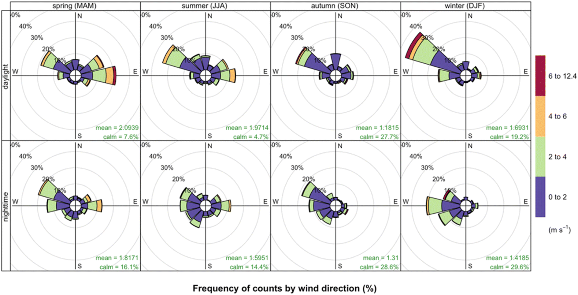

Fig. 3 Seasonal Wind Rose based on the hourly mean wind speed and wind direction of Modena.

2.4 Calibration model setup

To estimate the atmospheric concentration from the data provided by the sensor units a calibration model is needed. The cell's manufacturer provided a linear calibration equation to convert the voltage readings to the concentration of the target gas. These calibration models are derived from tests under lab conditions and previously shown to have modest performance in several outdoor applications.^20,32

Prior to the deployment of the units across town for air quality monitoring, an investigation of the best suitable calibration model configuration was performed on an initial co-location period concurrent for all LCSs. According to previous successful experience,¹⁴ for the current study Random Forest (RF)²⁵ was the algorithm chosen to build the calibration function. RF is a collection of decision trees generated using a random subset from the training data, where each level in the tree splits the dataset into smaller and smaller subsets to predict the target value. The split process ends when there are no further improvements in the model performance, or a minimum number of values have been reached. The final forest is the collection of all the trees acquired, and thus, when a calibration value is needed, the algorithm returns the mean estimate by all trees.

RF requires the selection and optimization of several hyperparameters. In this study two hyperparameters were explored: the number of trees (nT) and the lowest number of data points in a node (nN). The best suitable values for both hyperparameters were estimated by exploring RF performance across their parameter space, i.e. by performing RF simulations for possible values of the two hyperparameters, specifically between 100 and 20 000 for the number of trees and from 1 to 100 for the minimum number of data points. These tests were performed for all the units and all air pollutants, using the Spearman rank correlation coefficient as a performance index (see the Calibration model performance). Finally, the best set for both nT and nN was 1500 and 10, respectively, and these values were applied throughout the operation of the units and for all low-cost sensors used.

RF was found to provide satisfactory calibration results for amperometric gas sensors.^13,14,18 A useful advantage is the ability to inherently calculate the importance of each input variable.³³ This quantification is called Feature Importance (FI), with the term ‘feature’ indicating an input variable. FI allows for a more informed decision on which variables are important. RF and FI do not isolate the influence of each regression parameter. In order to reach the most suitable calibration model for the current application, we started from an initial extensive regression model, exploiting all variables available, and progressively reduced the number of regressors, based on the influence of each of them in the final calibration model according to FI. This can only help in understanding the current situation, not replace the chemical and physical processes that affect the air pollutant real concentrations.

FI is initially computed on each node of the tree, i.e. at each split of the branch, according to the following: FI for each node is the difference between the number of values in the node multiplied by their variance and the number of observations multiplied by their variance for each of the child nodes. Next, the mean FI for all the tree nodes is calculated, which is then normalized by the sum of all the FIs in the tree. The complete forest feature importance is the sum of the FIs in each tree for each feature divided by the number of trees. Finally, since this estimation method for the FI is biased,³³ FI permutation was used, i.e. the importance of a feature is calculated by randomly permutating one of the input variables, chosen at random.³³ It is defined as the difference between the original value of the accuracy index (variance in the inherent FI) and the reduction obtained after permutation. That is, in this method the FI can be calculated by using any accuracy index and not only variance. This process was automatically repeated 10 times to improve the FI robustness.

2.5 Calibration model performance

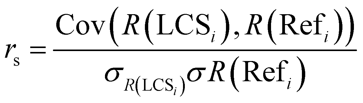
When assessing the calibration accuracy of nonlinear calibration algorithms, it is advisable to use a nonlinear correlation coefficient as well. Since the Pearson's correlation coefficient (r) is strictly valid for linear correlations,^7,34–36 in this study the correlation between the result of the calibration algorithm and the observations used the Spearman rank coefficient (r_s) which allows the assessment of the correlation between non-linear monotonic functions. r_s was also used as the statistical parameter in the FI estimates. Several other descriptive statistical parameters were also calculated as indicators for calibration accuracy, but for the sake of simplicity, only some selected statistical parameters are presented below, as the most useful for this study. The statistical analysis performed included the statistical parameters previously mentioned as well as a so-called “threshold” concentration (C_thrs). C_thrs was derived by a binned regression between the AQM observations and the corresponding values by the low-cost unit, allowing a 25% bias similarly to previous studies.¹⁴ Sample binned scatter plots are presented in Fig. 4, from co-location at MO_PF: they describe, for each 1 μg m⁻³ concentration bin in the MO_PF observations, the corresponding values in the LCS. The median and the 5 and 95 percentiles were also shown, along with the 1 : 1 line and its ±15% and ±25% bias: C_thrs is the lowest level for which the 5–95 percentile range of the sensor response is within the 25% bias. It is worth noting that the C_thrs refers to single (i.e. hourly) observations, i.e. aggregated statistics of sensor's response are better represented by the median LCS observations shown in Fig. 4, which are well in line with the AQM also at levels well below C_thrs.

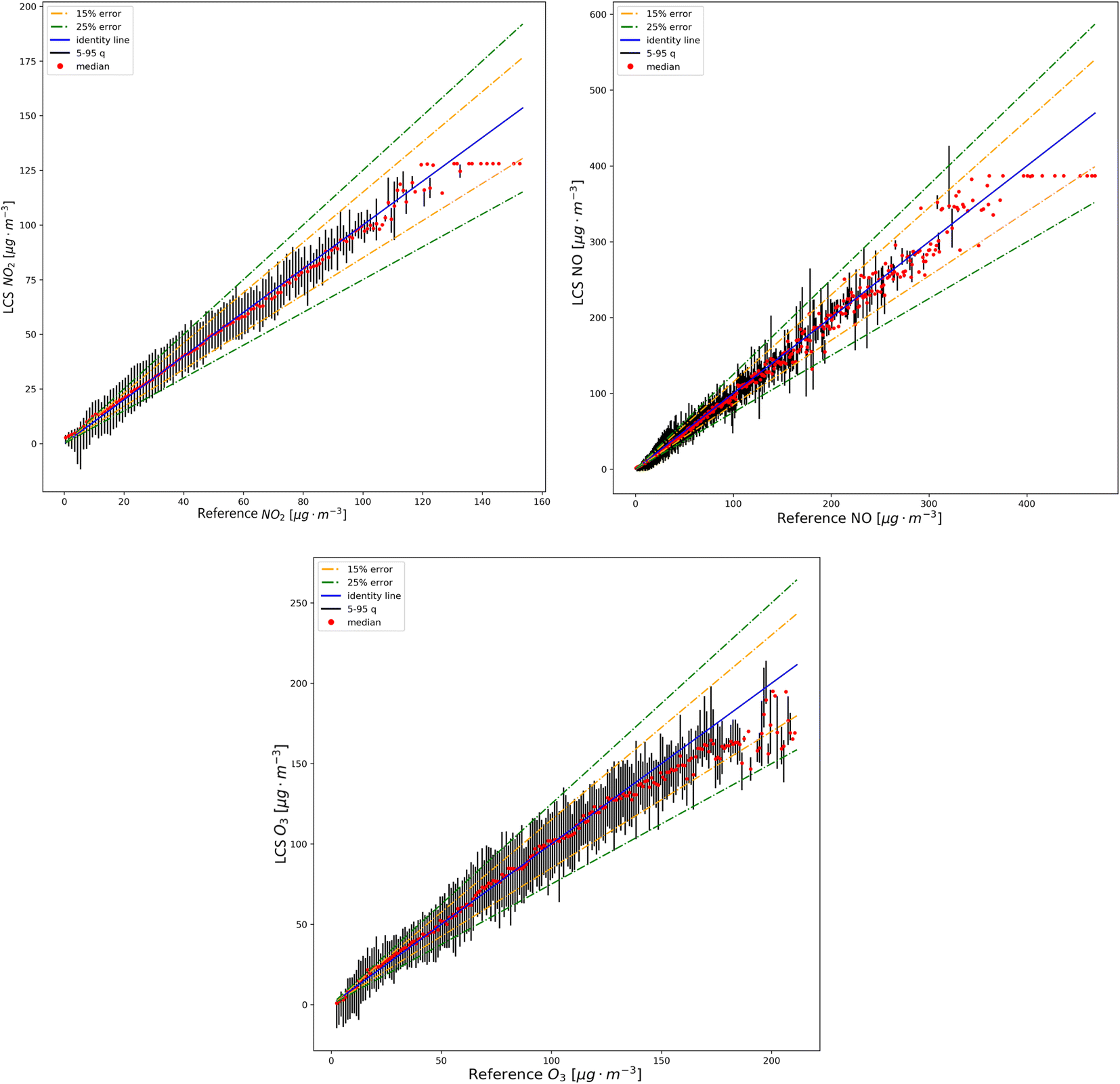Fig. 4 Binned regression between the AQM observations and the corresponding values from the low-cost sensor.

All the other statistical parameters used for this statistical assessment are mean absolute error (MAE), Root Mean Square Error (RMSE), and Spearman rank correlation (r_s) which are calculated, as follows:

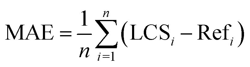
where LCS_i: the predicted value for the ith sample from the LCS. Ref_i: the reference value for the ith sample from the reference station. n: the total number of samples. R(LCS_i): the rank of the LCS data for the ith sample. R(Ref_i): the rank of the reference data for the ith sample. Cov(R(LCS_i)), R(Ref_i): the covariance between the ranks of the LCS and the reference data. σ_(R(LCSi): the standard deviation of the ranks of the LCS data. σ_(R(Refi): the standard deviation of the ranks of the reference data.

The coefficient of determination (r²) was also computed to visualize the variance between the LCS and AQM measurements (Fig. S1†). Prior to calibration, all missing values from the AQM, LCS and AQM concentration values below 0.1 μg m⁻³ (to exclude values below the limit of detection) were removed from the dataset. A cross-validation approach was applied to assess all the tested calibration models: the data collected and used for calibration was split randomly into two groups, containing 80% and 20% of the data, respectively. The former was used to train the calibration model and the latter to validate the calibration for the same period. All cells had an initial common training by co-location at MO_PF for 6 weeks (19 Aug – 30 Sept 2019) and validated by relocation at MO_VG (4 Oct – 15 Oct 2019). It is worth noting that O₃ is available only at MO_PF, i.e. the validation/relocation is possible only for NO_x.

The values of MAE, RMSE, r_s, r and C_thrs are listed in Table 2.

Table 2 Mean statistical performance indices for the calibration model applied in the study

Pollutant	MAE (μg m^−3)	RMSE (μg m^−3)	r s	r	C thrs (μg m^−3)
NO	4.15	10.14	0.82	0.95	∼50
NO2	5.64	8.86	0.88	0.89	∼40
O3	9.90	24.82	0.95	0.85	∼50

---

The analysis of the FI for model configuration featuring a large number of regressors showed some interesting patterns, as the large importance of NO_2,WE and NO_2,AUX cells in the prediction of NO. One possible reason for this behaviour, which was observed also in other studies (e.g. Bigi et al., 2018),¹⁴ might be linked to the NO-NO₂ photocatalytic cycle,³⁷ where NO is oxidized to NO₂ by O₃. If this is the case, it would imply that NO₂ is used as a proxy for NO. Moreover, in this same model configuration, the importance of NO₂ cell electrodes in NO prediction was large for all sensor units, while, in contrast, the NO electrodes were not contributing to the prediction of NO₂. Including NO_2,WE and NO_2,AUX in the calibration model of the NO cell improves its performance, but it is hardly justified by the expected working principle of the amperometric cell. This problem was unsolved, and the model with a simple configuration was used for NO henceforth, as well as for NO₂ and O₃, in order to keep a model consistent with the expected behaviour of the cell, with the aim to produce a more portable solution, although this leads to a lower performance. Therefore, the model configuration which was finally chosen, as the most suitable for the current application, was the following: for nitric oxide we relied on NO_WE and NO_AUX, for nitrogen dioxide on NO_2,WE and NO_2,AUX and for ozone on NO_2,WE, NO_2,AUX, O_x,WE and O_x,AUX, since the cell O_x-B431 is sensitive to both NO₂ and O₃.⁹

This latter calibration model setup was applied to all LCSs. The data presented in this study proceed from a comprehensive calibration including all co-location data collected throughout the study at MO_PF, in order to exploit all available information: this differs from the day-by-day operation of the network, when intermediate calibrations were regularly updated and the training dataset was periodically expanded by a sensor rotation of about 2–3 month deployment in the network and 3–4 weeks of deployment at MO_PF. The RF hyperparameters were not changed throughout the operation of the network, ensuring a smooth transition between calibrations/deployments. The data presented therefore correspond to the last calibration dataset used in the network operation, minimising the so-called “conceptual drift”²²i.e. the degradation of sensor performance due to the progressive unfitness of the calibration space for the observation space.

The operational calibration degraded over time with a rate dependent on the sensor unit, the compound. This degradation depended also on the calibration iteration: since the calibration dataset was progressively incremented during the operation of the network, the degradation of the performance either decreased slightly and/or stabilised, still depending on the sensor unit and the compound.³⁸ To test the performance of the LCS, during the network operation some LCSs were temporarily installed at GIA, next to the urban traffic AQM MO_VG, which was not used to build the calibration model. The RMSE resulting from these re-location activities was fairly steady throughout the study period and ranges between 10.3 and 11.0 μg m⁻³, for a 59 day relocation in 2020, to 11.7 μg m⁻³ for a 88 day relocation over 2021, in line with other literature studies, e.g. Karagulian et al.⁷ Fig. S2† shows the daily mean concentrations from the reference urban background station and the different LCSs that rotated through the same location (PFR) during the measurement period. It shows that the LCS network captures similar temporal variations and effectively differentiates between pollution levels and seasonality trends with the AQM.

All data analysis presented was performed using statistical software R.³⁹

3 Results and discussion

3.1 Patterns

The complete time series of 7- day averages at all locations for the 3 investigated pollutants is presented in Fig. 5.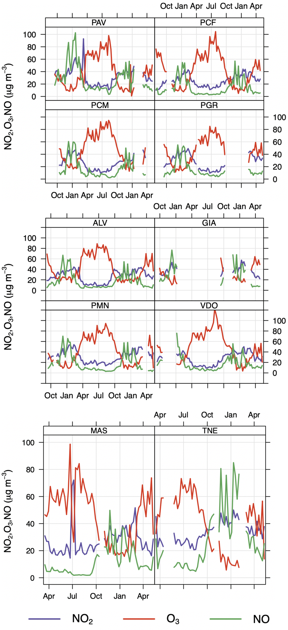

Fig. 5 Time-series of temporal variations of trace gases in Modena during the measurement period.

O₃ exhibited a strong seasonality, featuring higher mean values in the summer at all sites (∼75.4 μg m⁻³) and lower levels in winter (∼20 μg m⁻³), although some differences in O₃ levels across the locations occurred. During the summer months, the night-time (1:00–3:00) O₃ values were mostly homogeneous among all locations at ∼50 μg m⁻³. The mean seasonal O₃ differences are large in the winter and summer months in Modena (ΔO₃ = 56.9 μg m⁻³). Day-time values differed occasionally within the various locations in the city. In Modena, VDO (a suburban street) exhibited the highest O₃ levels in the entire study. It should be noted that these mean values were close to reaching the O₃ regulation of 180 μg m⁻³.

There is evidence of intra-urban variability in NO₂, NO, and O₃ concentrations between different sites in the city. For example, in 2019, PFR had a mean NO₂ concentration of 17.2 μg m⁻³, while PMN had a mean NO₂ concentration of 34.6 μg m⁻³, which is nearly double, consistent with their urban background and urban traffic pollution conditions respectively. To understand O₃ intra-urban variability, we focussed on 2020 since there is a full coverage of the summer months. For instance, VGI had a low concentration of O₃ mean (standard deviation) 25.0 (21.6), whereas PCU had a high ozone concentration of 54.2 (34.1) μg m⁻³, which indicates a potentially elevated level of ozone pollution within the hospital environment. Considering seasonality means between two urban zones in Modena, PGR which is an urban low emission zone had a mean (sd) NO₂ concentration of 43.2 (14.0) μg m⁻³ in the winter whereas PMN which is an urban traffic zone also had a similar NO₂ concentration of 43.1 (15.8) μg m⁻³ in the winter. The winter season in TNE recorded the highest levels of NO and NO₂ at 55.5 μg m⁻³ and 42.8 μg m⁻³, respectively, with lower levels of O₃ at 11.2 μg m⁻³.

The diurnal patterns for the three pollutants are presented in Fig. 6. Prior to computing these diurnal means, depending on how many missing values were present, we dealt with the missing data with one of the two following methods – (1) in the case of more than 10 hours of missing data, that day was removed and (2) in the case of less than 10 hours of missing data, we used mean imputation. For example, if a 4:00 reading was missing on a Monday, these data were replaced by the mean of all readings from all sensors taken on Monday at 4:00.

Fig. 6 Average diurnal time-series of trace gases including all locations during the measurement period.

At almost all the locations, NO₂ exhibits morning and afternoon peaks during rush hours. These peaks differ in absolute concentration, in duration and in contrast with night-time values. As shown in Fig. 6, the NO and NO₂ levels were considerably greater on weekdays than on weekends, because of the difference in the volume of vehicular traffic. Additionally, during weekdays, NO₂ experienced a larger mean than NO. This is due to NO₂'s longer lifespan and the NO's greater reactivity.

On weekdays the diurnal cycle of NO features two peaks, with the magnitude of the morning peak (∼43 μg m⁻³) being greater than that of the evening peak (∼34 μg m⁻³), while for NO₂ the evening peak was higher (∼42 μg m⁻³). NO decreases after its morning high (08:00 LT) and reaches its lowest level around 13:00 LT. A rise in O₃ is concurrent with a decrease in NO and NO₂, as well. The shallow night-time planetary boundary layer (NPBL), often followed by a temperature inversion, limits the dispersion of surface NO emissions and contributes to the second peak in NO between 19:00 and 20:00 LT. Cities throughout the world exhibit this pattern in the temporal variability of air pollution.⁴⁰ Local air circulations or short-term meteorological effects can occasionally have an impact on variations,³⁹ but the fundamental pattern tends to be highly similar. According to background air pollution, specific emission conditions, general weather conditions and concentrations vary in different cities.

The diurnal cycle of ozone concentration typically has higher concentrations during the day and lower amounts at night. After the sun rises, the ozone concentration gradually rises, reaches its peak during the day, and then gradually falls until the next morning. Meteorological conditions and photochemical activity are the main causes of this variability. In summer in Modena the global solar radiation and the height of the mixing layer rise between 08:00 LT and 14:00–15:00 LT, contributing to a dilution of NO_x emissions and triggering the photolysis of NO₂ and the formation of O₃.⁴¹ O₃ and a significant portion of NO₂ are secondary contaminants that are created as a result of a series of complex reactions, whereas NO is a primary contaminant. Solar radiation fuels several photochemical processes as early as at 07:00 in summer months: in the photostationary cycle, occurring mainly during daytime, O₃ oxidises NO to NO₂, which is photolysed back to NO regenerating O₃. This cycle contributes to the explanation of the drop in O₃ levels in the early morning, concurrently to the peak in NO concentration. The height of the mixing layer over the city is another element that affects air pollution concentrations. On a clear day, contaminants present within the NPBL during the night will be diluted along with daytime emissions as the mixing layer rises during the day.

The average maximum value of O₃ was higher on the weekends than it was during the weekdays. This pattern of temporal variability, which is known as the weekend effect mechanism, is also prevalent in other cities. It includes (i) a decrease in weekend NO_x emissions paired with the susceptibility of ozone generation to VOC concentration, (ii) a variation in the timing of NO_x emissions, and (iii) a carryover of O₃ and precursor concentrations on Friday and Saturday evenings. The weekend impact can therefore be partially explained by the following mechanism: because there is less NO emission on weekends in the morning, there is a limit to how much O₃ can be depleted during the day, leading to an accumulation of O_3.

3.2 Air pollution hotspots

LCSs allowed the identification of intra-urban variability and air pollution hotspots within the town. Any location with values (Table 3) above the EU regulation (Directive 50/2008) was examined and analyzed. In Modena both NO₂ and O₃ hotspots were detected.

Table 3 Mean and standard deviation (μg m⁻³) values for NO₂, NO and O₃ in all the locations of Modena during the measurement period

Monitoring location	NO2 (mean, SD) μg m^−3	NO (mean, SD) μg m^−3	O3 (mean, SD) μg m^−3
PFR	2019 ∼ 17.2, 12.7	2019 ∼ 7.99, 17.2	2019 ∼ 56.2, 39.6
	2020 ∼ 24.3, 16.1	2020 ∼ 14.0, 27.9	2020 ∼ 50.5, 42.9
	2021 ∼ 36.3, 15.8	2021 ∼ 16.4, 24.0	2021 ∼ 24.7, 25.2
PGR	2019 ∼ 31.6, 12.6	2019 ∼ 19.9, 28.0	2019 ∼ 27.3, 24.3
	2020 ∼ 23.5, 16.6	2020 ∼ 13.9, 21.8	2020 ∼ 52.9, 32.4
	2021 ∼ 36.6, 14.1	2021 ∼ 9.75, 10.4	2021 ∼ 45.1, 23.2
PCM/PCU	2019 ∼ 32.2, 13.9	2019 ∼ 25.0, 35.8	2019 ∼ 29.7, 19.1
	2020 ∼ 23.7, 18.5	2020 ∼ 15.6, 33.2	2020 ∼ 54.2, 34.1
	2021 ∼ 38.6, 16.3	2021 ∼ 14.0, 25.4	2021 ∼ 28.4, 17.9
PAV	2019 ∼ 34.9, 17.3	2019 ∼ 40.0, 55.5	2019 ∼ 21.4, 23.1
	2020 ∼ 32.1, 23.4	2020 ∼ 29.6, 33.5	2020 ∼ 43.9, 41.7
	2021 ∼ 30.5, 16.3	2021 ∼ 15.8, 23.5	2021 ∼ 37.1, 29.9
PMN	2019 ∼ 34.6, 13.9	2019 ∼ 29.7, 36.2	2019 ∼ 20.4, 22.6
	2020 ∼ 28.0, 18.1	2020 ∼ 16.7, 23.6	2020 ∼ 50.9, 41.3
	2021 ∼ 41.3, 15.2	2021 ∼ 18.2, 25.6	2021 ∼ 25.3, 28.1
ALV	2019 ∼ 28.2, 13.1	2019 ∼ 23.2, 35.6	2019 ∼ 31.7, 25.5
	2020 ∼ 23.6, 17.1	2020 ∼ 17.2, 29.4	2020 ∼ 48.3, 35.9
	2021 ∼ 34.5, 14.6	2021 ∼ 14.5, 21.9	2021 ∼ 37.6, 32.6
GIA	2019 ∼ 35.2, 16.6	2019 ∼ 30.5, 41.6	2019 ∼ 27.5, 23.4
	2020 ∼ 40.6, 15.3	2020 ∼ 41.1, 48.5	2020 ∼ 25.0, 21.6
	2021 ∼ 37.0, 19.0	2021 ∼ 19.1, 31.9	2021 ∼ 38.6, 28.3
VDO	2019 ∼ 28.7, 16.1	2019 ∼ 21.0, 31.1	2019 ∼ 45.7, 31.2
	2020 ∼ 24.5, 16.5	2020 ∼ 16.3, 28.4	2020 ∼ 58.9, 42.3
	2021 ∼ 36.4, 16.6	2021 ∼ 16.7, 23.9	2021 ∼ 28.4, 29.3
MAS	2020 ∼ 25.2, 20.5	2020 ∼ 9.13, 18.5	2020 ∼ 51.6, 38.5
	2021 ∼ 30.2, 16.5	2021 ∼ 15.3, 25.3	2021 ∼ 38.9, 32.9
TNE	2020 ∼ 31.3, 23.1	2020 ∼ 22.8, 39.1	2020 ∼ 44.8, 37.8
	2021 ∼ 38.3, 21.7	2021 ∼ 36.4, 47.8	2021 ∼ 33.1, 35.8

---

In Modena, 9 out of 10 locations had O₃ 8 hour hotspots. The one exception was VIG, which is facing a major urban road with high NO₂. Out of all the others, VDO had the highest values and highest number of days for a local O₃ hotspot. Indeed, some of these values almost reached the O₃ 1 hour regulation of 180 μg m⁻³. Only three locations exceeded the 1 hour regulation: PFO, PMN, and VDO. In both PFO and PMN, only one O₃ exceedance was observed, and it occurred between July and August. While in VDO, several exceedances were identified for August and one in the beginning of September. The VDO site is at the crossing of a dead-end street in a small neighbourhood featuring small buildings allowing for an unobstructed air flow, and little to no traffic. However, the VDO location is about 250 m away from the ring road, which runs elevated several meters above ground. The highest mean NO₂ values were observed at the two traffic locations (GIA and TNE); consistently these locations also had the largest NO levels, along with PAV, probably because of the large traffic on the road facing the LCS.

4 Conclusions

This work aimed at assessing the performance of a network of 12 low-cost sensor units in monitoring NO, NO₂ and O₃ levels in Modena, one of a highly polluted cities in the Po valley (Northern Italy), a European air pollution hotspot. Initially in order to calibrate these units, an extensive analysis of the selected calibration protocols was performed, based on the Random Forest (RF) algorithm. Several stages of calibration were examined: available input variables to be used (provided by all low cost sensors installed in the same unit), several detailed analyses of their significance in each pollutant calibration performance, and the specific influence of meteorological parameters on calibration validation.

Following a 20 month field campaign, the effectiveness of the low-cost sensors was assessed by the analysis of the concentration patterns collected and by comparison with local reference air quality stations. The statistical performance metrics showed a little decline in comparison to the calibration periods, but overall accuracy was still satisfactory. The measuring trial, which required a remarkably long time for these kinds of sensors, revealed that the low-cost sensors in particular displayed a low amount of drift. The results of the investigation demonstrated that the low-cost sensors could replicate the typical temporal variability of the monitored pollutants.

According to the findings, the intra-urban variability of NO₂, NO, and O₃ concentrations has been observed in different sites in the city of Modena. The mean concentration of these pollutants varies greatly between sites, with some areas having nearly double the concentration of others. The summer months showed variability in O₃ concentration, with some sites having a potentially elevated level of ozone pollution. Seasonality also influences the NO and NO₂ concentration, with the winter season recording the highest levels of the pollutants in some urban zones. The pollutant levels in Modena showed a clear pattern with higher levels of NO and NO₂ and lower levels of O₃ on weekdays compared to weekends. The diurnal cycle of NO and NO₂ showed morning and afternoon peaks during rush hours and were influenced by the volume of vehicular traffic. In contrast, the diurnal cycle of O₃ showed higher levels during the day and lower levels at night and was influenced by meteorological conditions and photochemical activity. The levels were also affected by local air circulations and short-term meteorological effects.

The study's findings showed that low-cost sensors can be a useful addition to reference air quality measurements since they allow for greater spatial coverage and the monitoring of pollutant concentrations: if correctly handled they can provide valuable information to local authorities and to the population regarding air quality variability and support improved environmental policies and actions. The study also emphasized that this type of sensor management requires expertise in order to monitor the calibration's quality and identify potential problems. Implementing an automated data quality procedure in particular will help identify any drifts early on. This study also shows that using a machine learning approach, such as RF, it is possible to calibrate both NO₂ and O₃ keeping a satisfactory and steady performance in several validation scenarios. This is especially true for NO₂ since its estimated concentration seems not to be significantly influenced by other electrochemical sensors or by meteorology. For NO, longer calibration periods could improve the LCS performance, because of the large reactivity of this compound, also because the reference AQM was a site under urban background conditions. However, for all air pollutants, the co-location period of each low-cost sensor at the AQM for calibration should include the concentration range expected at the area of future low-cost sensor deployment, for instance, based on the historical data from other AQMs in the same area.

Conflicts of interest

There are no conflicts to declare.

Acknowledgements

This study was supported by the project TRAFAIR Understanding Traffic Flow to Improve Air Quality under the grant: 2017-EU-IA-0167 and co-financed by the Connecting Europe Facility of the European Union. The authors thank the DBgroup of University of Modena and Reggio Emilia for the maintenance of the database storing the sensor data.

References

1. P. Kumar, L. Morawska, C. Martani, G. Biskos, M. Neophytou, S. Di Sabatino, M. Bell, L. Norford and R. Britter, Environ. Int., 2015, 75, 199–205.
2. C. Borrego, A. M. Costa, J. Ginja, M. Amorim, M. Coutinho, K. Karatzas, T. Sioumis, N. Katsifarakis, K. Konstantinidis, S. De Vito, E. Esposito, P. Smith, N. André, P. Gérard, L. A. Francis, N. Castell, P. Schneider, M. Viana, M. C. Minguillón, W. Reimringer, R. P. Otjes, O. von Sicard, R. Pohle, B. Elen, D. Suriano, V. Pfister, M. Prato, S. Dipinto and M. Penza, Atmos. Environ., 2016, 147, 246–263.
3. O. A. M. Popoola, D. Carruthers, C. Lad, V. B. Bright, M. I. Mead, M. E. J. Stettler, J. R. Saffell and R. L. Jones, Atmos. Environ., 2018, 194, 58–70.
4. E. S. Cross, L. R. Williams, D. K. Lewis, G. R. Magoon, T. B. Onasch, M. L. Kaminsky, D. R. Worsnop and J. T. Jayne, Atmos. Meas. Tech., 2017, 10, 3575–3588.
5. A. Larkin, J. A. Geddes, R. V. Martin, Q. Xiao, Y. Liu, J. D. Marshall, M. Brauer and P. Hystad, Environ. Sci. Technol., 2017, 51, 6957–6964.
6. G. Veratti, S. Fabbi, A. Bigi, A. Lupascu, G. Tinarelli, S. Teggi, G. Brusasca, T. M. Butler and G. Ghermandi, Atmos. Environ., 2020, 223, 117285.
7. F. Karagulian, M. Barbiere, A. Kotsev, L. Spinelle, M. Gerboles, F. Lagler, N. Redon, S. Crunaire and A. Borowiak, Atmosphere, 2019, 10, 506.
8. R. Baron and J. Saffell, ACS Sens., 2017, 2, 1553–1566.
9. M. Hossain, J. Saffell and R. Baron, ACS Sens., 2016, 1, 1291–1294.
10. M. Levy Zamora, C. Buehler, H. Lei, A. Datta, F. Xiong, D. R. Gentner and K. Koehler, ACS ES&T Engineering, 2022, 2, 780–793.
11. D. Margaritis, C. Keramydas, I. Papachristos and D. Lambropoulou, Aerosol Air Qual. Res., 2021, 21, 210073.
12. H. Omidvarborna, P. Kumar and A. Tiwari, Atmos. Environ., 2020, 223, 117264.
13. N. Zimmerman, A. A. Presto, S. P. N. Kumar, J. Gu, A. Hauryliuk, E. S. Robinson, A. L. Robinson and R. Subramanian, Atmos. Meas. Tech., 2018, 11, 291–313.
14. A. Bigi, M. Mueller, S. K. Grange, G. Ghermandi and C. Hueglin, Atmos. Meas. Tech., 2018, 11, 3717–3735.
15. C. Malings, R. Tanzer, A. Hauryliuk, S. P. N. Kumar, N. Zimmerman, L. B. Kara, A. A. Presto and R. Subramanian, Atmos. Meas. Tech., 2019, 12, 903–920.
16. G. Miskell, J. A. Salmond and D. E. Williams, ACS Sens., 2018, 3, 832–843.
17. D. H. Hagan, G. Isaacman-Vanwertz, J. P. Franklin, L. M. M. Wallace, B. D. Kocar, C. L. Heald and J. H. Kroll, Atmos. Meas. Tech., 2018, 11, 315–328.
18. S. Vikram, A. Collier-Oxandale, M. H. Ostertag, M. Menarini, C. Chermak, S. Dasgupta, T. Rosing, M. Hannigan and W. G. Griswold, Atmos. Meas. Tech., 2019, 12, 4211–4239.
19. J. Gordon Casey and M. P. Hannigan, Atmos. Meas. Tech., 2018, 11, 6351–6378.
20. K. R. Smith, P. M. Edwards, P. D. Ivatt, J. D. Lee, F. Squires, C. Dai, R. E. Peltier, M. J. Evans, Y. Sun and A. C. Lewis, Atmos. Meas. Tech., 2019, 12, 1325–1336.
21. P. Wei, L. Sun, A. Abhishek, Q. Zhang, Z. Huixin, Z. Deng, Y. Wang and Z. Ning, Atmos. Environ., 2020, 230, 117509.
22. S. De Vito, E. Esposito, N. Castell, P. Schneider and A. Bartonova, Sens. Actuators, B, 2020, 310, 127869.
23. H. Kim, M. Müller, S. Henne and C. Hüglin, Atmos. Meas. Tech., 2022, 15, 2979–2992.
24. S. De Vito, E. Esposito, M. Salvato, O. Popoola, F. Formisano, R. Jones and G. Di Francia, Sens. Actuators, B, 2018, 255, 1191–1210.
25. L. Breiman, Mach. Learn., 2001, 45, 5–32.
26. D. R. Peters, O. A. M. Popoola, R. L. Jones, N. A. Martin, J. Mills, E. R. Fonseca, A. Stidworthy, E. Forsyth, D. Carruthers, M. Dupuy-Todd, F. Douglas, K. Moore, R. U. Shah, L. E. Padilla and R. A. Alvarez, Atmos. Meas. Tech., 2022, 15, 321–334.
27. M. A. Zaidan, Y. Xie, N. H. Motlagh, B. Wang, W. Nie, P. Nurmi, S. Tarkoma, T. Petaja, A. Ding and M. Kulmala, IEEE Sens. J., 2022, 1.
28. J. Kuula, H. Timonen, J. V. Niemi, H. E. Manninen, T. Rönkkö, T. Hussein, P. L. Fung, S. Tarkoma, M. Laakso, E. Saukko, A. Ovaska, M. Kulmala, A. Karppinen, L. Johansson and T. Petäjä, Atmos. Chem. Phys., 2022, 22, 4801–4808.
29. R. S. Sokhi, N. Moussiopoulos, A. Baklanov, J. Bartzis, I. Coll, S. Finardi, R. Friedrich, C. Geels, T. Grönholm, T. Halenka, M. Ketzel, A. Maragkidou, V. Matthias, J. Moldanova, L. Ntziachristos, K. Schäfer, P. Suppan, G. Tsegas, G. Carmichael, V. Franco, S. Hanna, J.-P. Jalkanen, G. J. M. Velders and J. Kukkonen, Atmos. Chem. Phys., 2022, 22, 4615–4703.
30. Inventario regionale emissioni in atmosfera (INEMAR) – Inventario emissioni INEMAR 2019 – Dati Arpae, https://dati.arpae.it/dataset/inventario-emissioni-aria-inemar/resource/d82aad00-2434-429e-b4dc-2304dc6244de, accessed 4 February 2023.
31. C. Barbieri, La qualità dell’aria in Provincia di Modena: report sintetico anno 2018, Modena, 2019.
32. C. Borrego, J. Ginja, M. Coutinho, C. Ribeiro, K. Karatzas, T. Sioumis, N. Katsifarakis, K. Konstantinidis, S. De Vito, E. Esposito, M. Salvato, P. Smith, N. André, P. Gérard, L. A. Francis, N. Castell, P. Schneider, M. Viana, M. C. Minguillón, W. Reimringer, R. P. Otjes, O. von Sicard, R. Pohle, B. Elen, D. Suriano, V. Pfister, M. Prato, S. Dipinto and M. Penza, Atmos. Environ., 2018, 193, 127–142.
33. A. Altmann, L. Toloşi, O. Sander and T. Lengauer, Bioinformatics, 2010, 26, 1340–1347.
34. L. Spinelle, M. Gerboles, M. G. Villani, M. Aleixandre and F. Bonavitacola, Sens. Actuators, B, 2015, 215, 249–257.
35. N. Castell, F. R. Dauge, P. Schneider, M. Vogt, U. Lerner, B. Fishbain, D. Broday and A. Bartonova, Environ. Int., 2017, 99, 293–302.
36. W. Jiao, G. Hagler, R. Williams, R. Sharpe, R. Brown, D. Garver, R. Judge, M. Caudill, J. Rickard, M. Davis, L. Weinstock, S. Zimmer-Dauphinee and K. Buckley, Atmos. Meas. Tech., 2016, 9, 5281–5292.
37. J. H. Seinfeld and S. N. Pandis, Atmospheric Chemistry and Physics: from Air Pollution to Climate Change, 2016.
38. G. D'Elia, M. Ferro, P. Sommella, S. De Vito, S. Ferlito, P. D'Auria and G. D. Francia, IEEE Trans. Instrum. Meas., 2022, 71, 1–11.
39. R Core Team, R: A Language and Environment for Statistical Computing. R Foundation for Statistical Computing, Vienna, Austria, 2021, https://www.R-project.org/.
40. M. L. Sanchez, B. de Torre, M. A. García and I. Pérez, Atmos. Environ., 2007, 41, 1302–1314.
41. A. G. Ulke and N. A. Mazzeo, Atmos. Environ., 1998, 32, 1615–1622.

---

Footnote

† Electronic supplementary information (ESI) available. See DOI: https://doi.org/10.1039/d2ea00165a

---