
 Open Access Article
 This Open Access Article is licensed under a Creative Commons Attribution-Non Commercial 3.0 Unported Licence
An analysis of degradation in low-cost particulate matter sensors†
Priyanka
deSouza
 *ab,
Karoline
Barkjohn
c,
Andrea
Clements
c,
Jenny
Lee
d,
Ralph
Kahn
e,
Ben
Crawford
f and
Patrick
Kinney
g
*ab,
Karoline
Barkjohn
c,
Andrea
Clements
c,
Jenny
Lee
d,
Ralph
Kahn
e,
Ben
Crawford
f and
Patrick
Kinney
g
aDepartment of Urban and Regional Planning, University of Colorado Denver, Denver, CO 80202, USA. E-mail: priyanka.desouza@ucdenver.edu
bCU Population Center, University of Colorado Boulder, Boulder, CO 80302, USA
cOffice of Research and Development, US Environmental Protection Agency, 109 T.W. Alexander Drive, Research Triangle Park, NC 27711, USA
dDepartment of Biostatistics, Harvard T.H. Chan School of Public Health, Boston, MA 02115, USA
eNASA Goddard Space Flight Center, Greenbelt, MD 20771, USA
fDepartment of Geography and Environmental Sciences, University of Colorado Denver, 80202, USA
gBoston University School of Public Health, Boston, MA 02118, USA
First published on 3rd February 2023
Abstract
Low-cost sensors (LCSs) are increasingly being used to measure fine particulate matter (PM2.5) concentrations in cities around the world. One of the most commonly deployed LCSs is PurpleAir with ∼15![[thin space (1/6-em)]](https://www.rsc.org/images/entities/char_2009.gif) 000 sensors deployed in the United States, alone. PurpleAir measurements are widely used by the public to evaluate PM2.5 levels in their neighborhoods. PurpleAir measurements are also increasingly being integrated into models by researchers to develop large-scale estimates of PM2.5. However, the change in sensor performance over time has not been well studied. It is important to understand the lifespan of these sensors to determine when they should be serviced or replaced, and when measurements from these devices should or should not be used for various applications. This paper fills this gap by leveraging the fact that: (1) each PurpleAir sensor is composed of two identical sensors and the divergence between their measurements can be observed, and (2) there are numerous PurpleAir sensors within 50 meters of regulatory monitors allowing for the comparison of measurements between these instruments. We propose empirically-derived degradation outcomes for the PurpleAir sensors and evaluate how these outcomes change over time. On average, we find that the number of ‘flagged’ measurements, where the two sensors within each PurpleAir sensor disagree, increases with time to ∼4% after 4 years of operation. Approximately, 2 percent of all PurpleAir sensors were permanently degraded. The largest fraction of permanently degraded PurpleAir sensors appeared to be in the hot and humid climate zone, suggesting that sensors in these locations may need to be replaced more frequently. We also find that the bias of PurpleAir sensors, or the difference between corrected PM2.5 levels and the corresponding reference measurements, changed over time by −0.12 μg m−3 (95% CI: −0.13 μg m−3, −0.10 μg m−3) per year. The average bias increases dramatically after 3.5 years. Further, climate zone is a significant modifier of the association between degradation outcomes and time.
000 sensors deployed in the United States, alone. PurpleAir measurements are widely used by the public to evaluate PM2.5 levels in their neighborhoods. PurpleAir measurements are also increasingly being integrated into models by researchers to develop large-scale estimates of PM2.5. However, the change in sensor performance over time has not been well studied. It is important to understand the lifespan of these sensors to determine when they should be serviced or replaced, and when measurements from these devices should or should not be used for various applications. This paper fills this gap by leveraging the fact that: (1) each PurpleAir sensor is composed of two identical sensors and the divergence between their measurements can be observed, and (2) there are numerous PurpleAir sensors within 50 meters of regulatory monitors allowing for the comparison of measurements between these instruments. We propose empirically-derived degradation outcomes for the PurpleAir sensors and evaluate how these outcomes change over time. On average, we find that the number of ‘flagged’ measurements, where the two sensors within each PurpleAir sensor disagree, increases with time to ∼4% after 4 years of operation. Approximately, 2 percent of all PurpleAir sensors were permanently degraded. The largest fraction of permanently degraded PurpleAir sensors appeared to be in the hot and humid climate zone, suggesting that sensors in these locations may need to be replaced more frequently. We also find that the bias of PurpleAir sensors, or the difference between corrected PM2.5 levels and the corresponding reference measurements, changed over time by −0.12 μg m−3 (95% CI: −0.13 μg m−3, −0.10 μg m−3) per year. The average bias increases dramatically after 3.5 years. Further, climate zone is a significant modifier of the association between degradation outcomes and time.
Environmental significanceLow-cost air quality sensors are widely used to fill in air quality monitoring gaps. However, little is known about the performance of these sensors over time. We evaluate degradation patterns across a network of widely-used low-cost particulate matter sensors, the PurpleAir. Overall, we find that 4% of measurements from PurpleAir sensors are degraded after 4 years of operation. Rates of degradation vary by climate zone. We also identify permanently degraded PurpleAir sensors that should be removed from operation. Our work provides a framework to quantify degradation in other low-cost air quality sensors. |
1 Introduction
Poor air quality is currently the single largest environmental risk factor to human health in the world,1–5 with ambient air pollution responsible for 6.7 million premature deaths every year.6 Accurate air quality data are crucial for tracking long-term trends in air quality levels, and for the development of effective pollution management plans. Levels of fine particulate matter (PM2.5), a criteria pollutant that poses more danger to human health than other widespread pollutants,7 can vary over distances as small as ∼10's of meters in complex urban environments.8–12 Therefore, dense monitoring networks are often needed to capture relevant spatial variations. U.S EPA air quality monitoring networks use approved Federal Reference or Equivalent Method (FRM/FEM) monitors, the gold standard for measuring air pollutants. However, these monitors are sparsely positioned across the US.13,14Low-cost sensors (LCSs) (<$2500 USD as defined by the U.S. EPA15) have the potential to capture concentrations of particulate matter (PM) in previously unmonitored locations and democratize air pollution information.13,16–21 Measurements from these devices are increasingly being integrated into models to develop large-scale exposure assessments.22–24
Most low-cost PM sensors rely on optical measurement techniques that introduce potential differences in mass estimations compared to reference monitors (i.e., FRM/FEM monitors).25–27 Optical sensor methods do not directly measure mass concentrations; rather, they measure light scattering of particles having diameters typically > ∼0.3 μm. Several assumptions are typically made to convert light scattering into mass concentrations that can introduce errors in the results. In addition, unlike reference monitors, LCSs do not dry particles before measuring them, so PM concentrations reported by LCSs can be biased high due to particle hygroscopic growth of particles when ambient relative humidity (RH) is high. Many research groups have developed different techniques to correct the raw LCS measurements from PM sensors. These models often include environmental variables, such as RH, temperature (T), and dewpoint (D), as predictors of the ‘true’ PM concentration.
However, little work has been done to evaluate the performance of low-cost PM sensors over time. There is evidence that the performance of these instruments can be affected by high PM events which can also impact subsequent measurements if the sensors are not cleaned properly.28 Although there has been some research evaluating drift in measurements from low-cost electrochemical gas sensors,29,30 there has been less work evaluating drift and degradation in low-cost PM sensors and identifying which factors affect these outcomes. An understanding of degradation could lead to better protocols for correcting low-cost PM sensors and could provide users with information on when to service or replace their sensors or whether data should or should not be used for certain applications.
This paper evaluates the performance of the PurpleAir sensor, one of the most common low-cost PM sensors over time. We chose to conduct this analysis with PurpleAir because:
(1) There is a sizable number of PurpleAir sensors within 50 meters of regulatory monitors that allows for comparison between PurpleAir measurements and reference data over time, and
(2) Each PurpleAir sensor consists of two identical PM sensors making it possible to evaluate how the two sensors disagree over time, and the different factors that contribute to this disagreement.
(3) Several studies have evaluated the short-term performance of the PurpleAir sensors at many different locations, under a variety of conditions around the world.31,32 However, none of these studies has evaluated the performance of the PurpleAir sensors over time. We aim to fill this gap.
2 Data and methods
2.1 PurpleAir measurements
There are two main types of PurpleAir sensors available for purchase: PA-I and PA-II. PA-I sensors have one PM sensor component (Plantower PMS 1003) for PM measurement. However, the PA-II PurpleAir sensor has two identical PM sensor components (Plantower PMS 5003 sensors) referred to as “channel A” and “channel B.” In this study, measurements were restricted to PA-II PurpleAir sensors in order to compare channels A and B. PA-II-Flex sensors (which use Plantower PMS 6003 PM sensors) were not included in this study as they were not made available until early 2022 after the dataset for this project was downloaded.The PA-II PurpleAir sensor operates for 10 s at alternating intervals and provides 2 min averaged data (prior to 30 May 2019, this was 80 s averaged data). The Plantower sensor components measure light scattering with a laser at 680 ± 10 nm wavelength 33,34 and are factory calibrated using ambient aerosol across several cities in China.27 The Plantower sensor reports estimated mass concentrations of particles with aerodynamic diameters < 1 μm (PM1), < 2.5 μm (PM2.5), and < 10 μm (PM10). For each PM size fraction, the values are reported in two ways, labeled cf_1 and cf_atm, in the PurpleAir dataset, which match the “raw” Plantower outputs.
The ratio of cf_atm and cf_1 (i.e. [cf_atm]/[cf_1]) is equal to 1 for PM2.5 concentrations below 25 μg m−3 (as reported by the sensor) and then transitions to a two-thirds ratio at a higher PM concentration (cf_1 concentrations are higher). The cf_atm data, displayed on the PurpleAir map, are the lower measurement of PM2.5 and are referred to as the “raw” data in this paper when making comparisons between initial and corrected datasets.33 When a PurpleAir sensor is connected to the internet, data are sent to PurpleAir's data repository. Users can choose to make their data publicly viewable (public) or control data sharing (private). All PurpleAir sensors also report RH and T levels.
For this study, data from 14927 PurpleAir sensors operating in the United States (excluding US territories) between 1 January 2017 to 20 July 2021 were downloaded from the API at 15-minute time resolution. A small number of PurpleAir sensors were operational before 2017. However, given that the number of PurpleAir sensors increased dramatically from 2017 onwards, we choose January 1 2017 as the start date of our analysis. Overall, 26.2% of dates had missing measurements, likely due to power outages or loss of WiFi that prevented the PurpleAir sensors from transmitting data. Of the sensors in our dataset, 2989 were missing channel B data, leaving us with 483511216 measurements from 11938 sensors with both channel A and B data. We removed all records with missing PM2.5 measurements in cf_1 channels A and B (∼0.9% of the data). We then removed all records with missing T and RH data (∼2.6% of all data). Of the non-missing records, all measurements where PM2.5 in cf._1 channels A and B were both >1500 μg m−3 were removed, as they correspond to conditions beyond the operating range of the PurpleAir sensor.25 We also removed measurements where T was ≤ −50 °C or ≥ 100 °C, or where RH was >99%, as these corresponded to extreme conditions (∼4.2% of all records). The remaining dataset contained 457488977 measurements from 11933 sensors.
The 15-minute data were averaged to 1 h intervals. A 75% data completeness threshold was used (at least 3 15minute measurements in an hour) based on channels A and B. This methodology ensured that the averages used were representative of hourly averages. We defined the hourly mean PM2.5 cf_1 as the average of the PM2.5 cf_1 measurements from channels A and B. We defined hourly mean PM2.5 cf_atm as the average of PM2.5 cf_atm measurements from channels A and B. We also calculated hourly mean T and RH from the 15 min averaged data from each PurpleAir sensor.
Overall, the dataset included 114259940 valid hourly averaged measurements with non-missing PM2.5 data in channels A or B corresponding to 11932 PurpleAir sensors (8312155 measurements from 935 indoor sensors and 105947785 measurements from 10997 outdoor sensors). A description of the number of sensors and measurements by the state is provided in Table S1 in the ESI.† (Fig. S1 in the ESI† displays the locations of indoor and outdoor PurpleAir sensors.) Of the 11932 PurpleAir sensors, 1377 (∼11.5%) had stopped reporting data at least a day before the data were downloaded (i.e., 20 July 2021), whereas the remaining sensors were still in operation (Fig. 1).
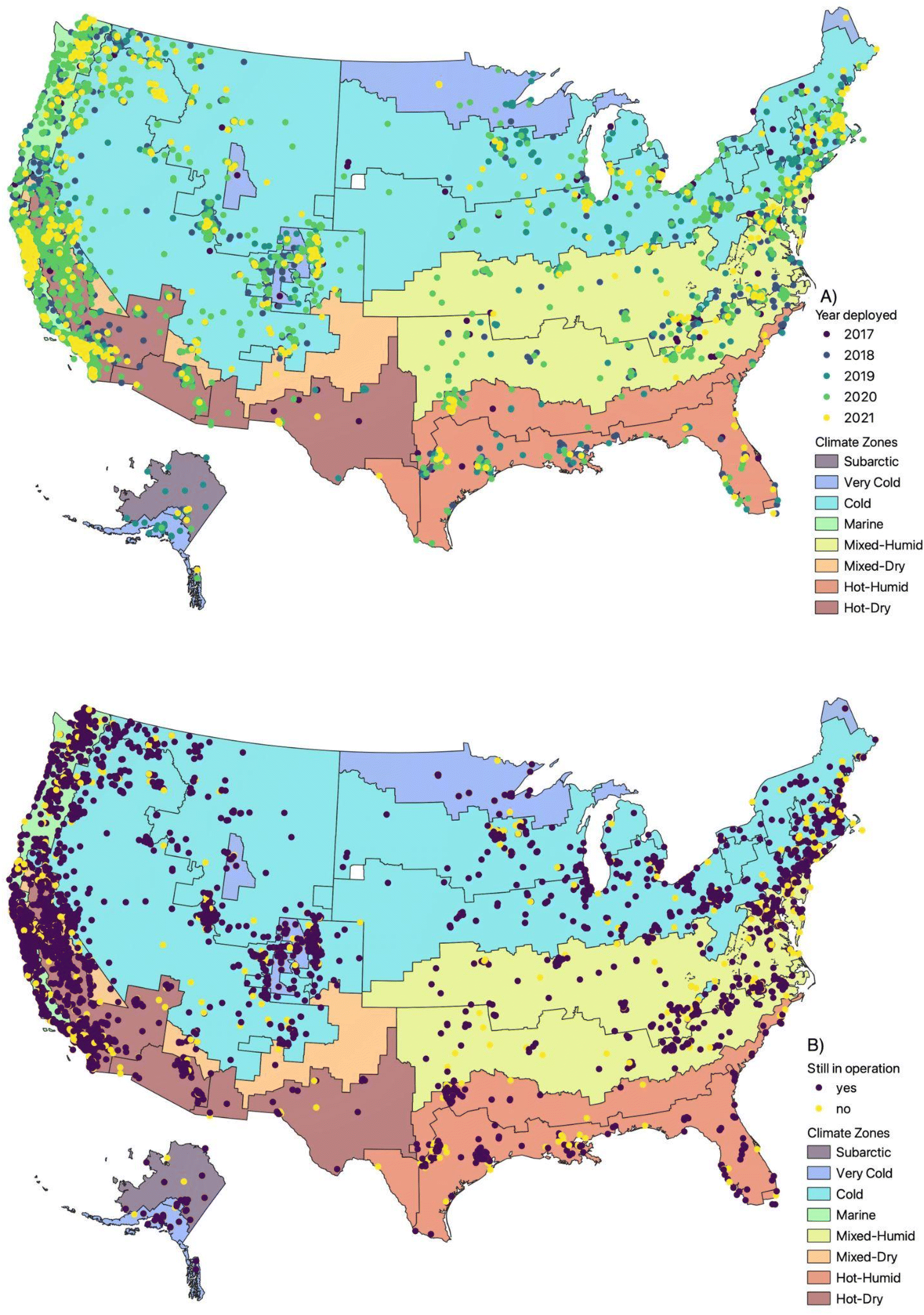 | ||
| Fig. 1 The distribution of PurpleAir sensors considered in this analysis (Hawaii is not displayed) depicting (A) the year each sensor was deployed, and (B) if the sensor was removed before 20 July 2021. Climate zones displayed are from the International Energy Conservation Code (IECC) climate zones (https://codes.iccsafe.org/content/IECC2021P1/chapter-3-ce-general-requirements, last accessed August 31, 2022). | ||
2.2 Reference measurements
Reference-grade (FRM/FEM) hourly PM2.5 measurements between 1 January 2017 and 20 July 2021 were obtained from 80 EPA Air Quality System (AQS) regulatory monitoring sites (https://www.epa.gov/aqs, last accessed August 31, 2022) located within 50 meters from any outdoor PurpleAir sensor (Table 1). At eight of the sites (located in Indiana, Iowa, Michigan, Tennessee, Virginia, and Washington), the monitoring method was updated midway during the period under consideration. Therefore, there were a total of 88 FRM/FEM monitors in our final analysis.| Monitors | State |
|---|---|

|
|
| 48 of the monitors in our sample were Met One BAM-1020 Mass Monitor w/VSCC – Beta Attenuation (1002533 merged measurements) |
33 reference monitors were in California (866197 merged measurements) |
| 9 were Met One BAM-1022 Mass Monitor w/VSCC or TE-PM2.5C – Beta Attenuation (218084 merged measurements) |
16 in Massachusetts (26930 merged measurements) |
| 10 were Teledyne T640 at 5.0 LPM – broadband spectroscopy (97706 merged measurements) |
9 in Washington (102382 merged measurements) |
| 8 were Teledyne T640× at 16.67 LPM – broadband spectroscopy (88040 merged measurements) |
5 in Tennessee (88505 merged measurements) |
| 6 were Thermo Scientific 5014i or FH62C14-DHS w/VSCC – Beta Attenuation (52116 merged measurements) |
4 in Virginia (33353 merged measurements) |
| 3 were Thermo Scientific TEOM 1400 FDMS or 1405 8500C FDMS w/VSCC – FDMS Gravimetric (21591 merged measurements) |
4 in Iowa (199138 merged measurements) |
| 2 were Thermo Scientific 1405-F FDMS w/VSCC – FDMS Gravimetric (15872 merged measurements) |
2 in Maine (8575 merged measurements) |
| 1 was GRIMM EDM Model 180 with Nafion dryer – Laser Light Scattering (1000 merged measurements) | 2 in Oregon (33554 merged measurements |
| 1 Was a Thermo Scientific Model 5030 SHARP w/VSCC – Beta Attenuation monitor (3199 merged measurements) | 2 in Indiana (26499 merged measurements) |
| 2 in Michigan (13678 merged measurements) |
|
| 1 each in Arizona (6045 merged measurements), Colorado (1000 merged measurements), Florida (15434 merged measurements), Nevada (17146 merged measurements), New Hampshire (30591 merged measurements), North Carolina (27253 merged measurements), South Dakota (1879 merged measurements), Texas (364 merged measurements), Wyoming (1618 merged measurements) |
|
2.3 Merging PurpleAir and reference measurements
We paired hourly averaged PM2.5 concentrations from 151 outdoor PurpleAir sensors with reference monitors that were within 50 meters. We removed records with missing EPA PM2.5 data or where reference PM2.5 measurements were <0. The dataset contained a total of 1500141 merged concentrations with non-missing PurpleAir and EPA PM2.5 values (Table 1).
If there was more than one reference monitor within 50 meters of a PurpleAir sensor, measurements were retained from one of the reference monitors. We prioritized retaining data from reference monitors that did not rely on light scattering techniques as these instruments tend to have an additional error when estimating aerosol mass.35
From the resulting dataset, we found that the Pearson correlation coefficient (R) between mean PM2.5 cf_1 and reference PM2.5 concentrations was 0.86, whereas the correlation between PM2.5 cf_atm and reference PM2.5 concentrations was 0.83. Henceforth, when describing PurpleAir measurements, we consider only the mean PM2.5 cf_1 concentrations.
2.4 Evaluating degradation
 standard deviations of the percentage difference between A and B for each PurpleAir sensor.33 The absolute difference of 5 μg m−3 was chosen to avoid excluding too many measurements at low PM concentrations, whereas defining a threshold based on the % difference between channels A and B was chosen to avoid excluding too many measurements at high concentrations.
A data-driven approach was adopted to determine if we should use a similar threshold in this study. We flagged measurements where the Δ > 5 μg m−3 and when the % difference between channels A and B was greater than the top percentile of the distribution of the % difference between A and B channels for each PurpleAir sensor. We allowed the percentile threshold to range from 0.0 to 0.99, by increments of 0.01. We use percentiles as a threshold instead of standard deviation as the % difference between the A and B channels is not normally distributed. At each step, we then compared the unflagged PurpleAir measurements with the corresponding reference data using the metrics: Pearson correlation coefficient (R) and the normalized root mean squared error (nRMSE). The percentile threshold that led to the best agreement between the PurpleAir sensor and the corresponding reference monitor was chosen. We calculated nRMSE in this study by normalizing the root mean square error (RMSE) by the standard deviation of PM2.5 from the corresponding reference monitor. As a sensitivity test, we repeated the above analysis after removing records where the reference monitor relied on a light scattering technique (namely the Teledyne and the Grimm instruments), thus eliminating the more error-prone data (Fig. S3†). We note that past studies have shown that the Beta-Attenuation Mass Monitors (BAM) are likely to experience more noise at low PM2.5 concentrations.35,36
After determining the threshold to flag measurements using the collocated data (Fig. 2), we evaluated the number of flagged measurements for each of the 11932 PurpleAir sensors in our sample. We propose the percentage of flagged measurements at a given operational time (from the time, in hours, since each sensor started operating) as a potential degradation outcome. To visually examine if a threshold value existed beyond which these outcomes increased significantly, we plotted this outcome as well as the percentage of cumulative flagged measurements over time (Fig. 3). We evaluated whether the distribution of PM2.5, RH, and T conditions for flagged measurements is statistically different from that for unflagged measurements (Table 2).
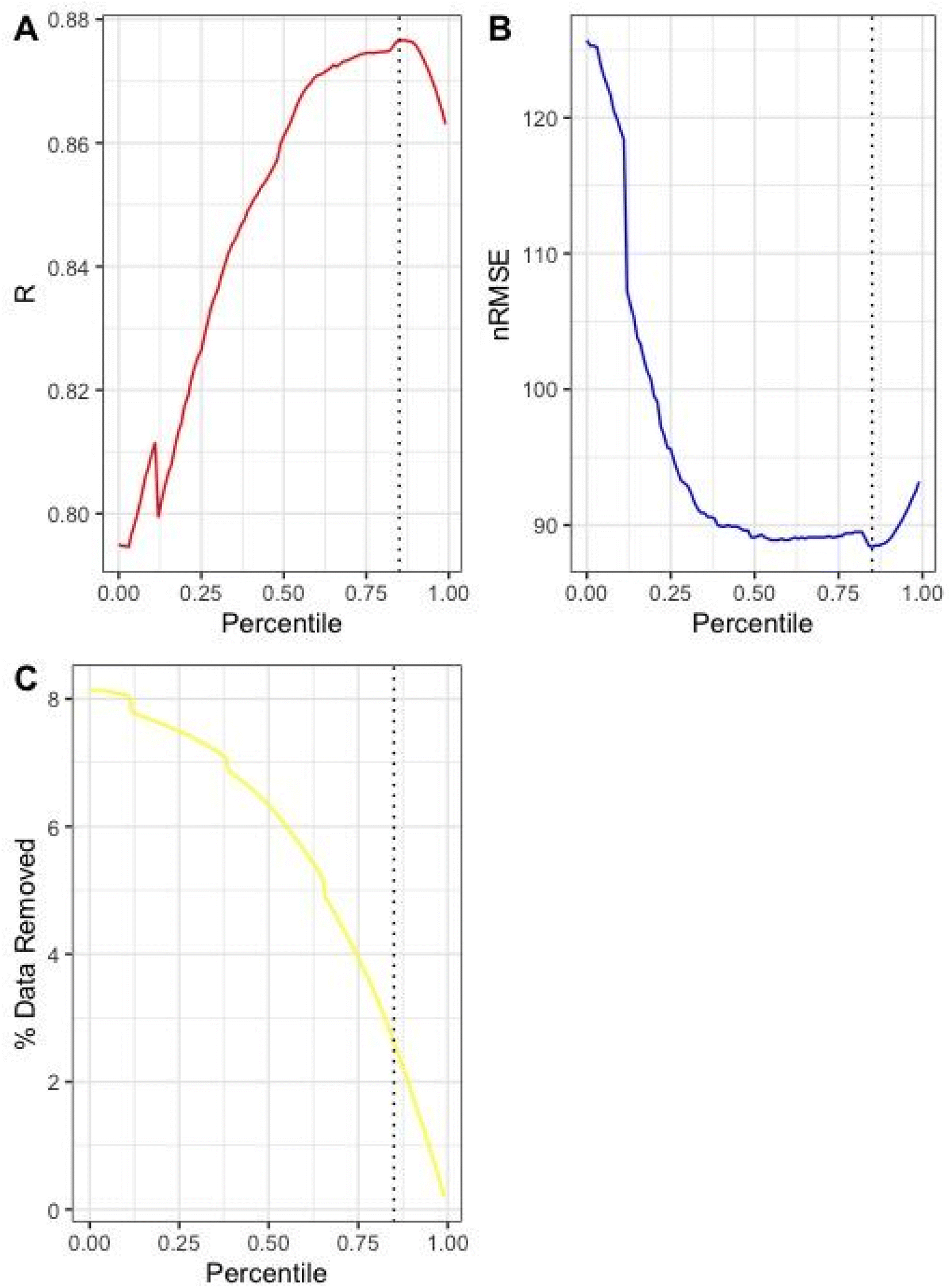 | ||
Fig. 2 : Agreement between the hourly PurpleAir measurements and the corresponding reference measurements, where measurements are flagged and removed based on the criterion: | channel A–channel B | > 5 μg m−3 and the % difference between channels A and B:  percentile of the percentage difference between A and B for each PurpleAir sensor, where we vary x between 0–0.99, captured by: (A) Pearson correlation coefficient (R), and (B) normalized root mean square error (nRMSE) metrics comparing unflagged measurements and the corresponding reference data based on different threshold percentile values. (C) The % of measurements that were removed (because they were flagged) when evaluating R and nRMSE, for different percentile thresholds applied to the data are also displayed. The dotted vertical line represents the 85th percentile which corresponds to the lowest nRMSE and the highest R. percentile of the percentage difference between A and B for each PurpleAir sensor, where we vary x between 0–0.99, captured by: (A) Pearson correlation coefficient (R), and (B) normalized root mean square error (nRMSE) metrics comparing unflagged measurements and the corresponding reference data based on different threshold percentile values. (C) The % of measurements that were removed (because they were flagged) when evaluating R and nRMSE, for different percentile thresholds applied to the data are also displayed. The dotted vertical line represents the 85th percentile which corresponds to the lowest nRMSE and the highest R. | ||
 | ||
| Fig. 3 Percentage of flagged PurpleAir measurements (yellow) and percentage of cumulative flagged (blue) measurements at a given operational time (time since each sensor started operation in hours) as well as the number of measurements recorded (red) plotted on the secondary y-axis on the right over all the PurpleAir sensors considered in this analysis. | ||
| Unflagged data (n = 112716535, 99%) |
Flagged data (n = 1543405, 1%) |
|
|---|---|---|
| Raw mean PM2.5 (mean of channel a and channel B) (μg m−3) | Min/max: 0/1459 | Min/max: 2.5/1339 |
| Mean: 10 | Mean: 26 | |
| Median: 5 | Median: 14 | |
| 1st Quartile: 2 | 1st Quartile: 7 | |
| 3rd Quartile: 11 | 3rd Quartile: 27 | |
| RH (%) | Min/max: 0/99 | Min/max: 0/99 |
| Mean: 46 | Mean: 43 | |
| Median: 48 | Median: 44 | |
| 1st Quartile: 34 | 1st Quartile: 30 | |
| 3rd Quartile: 59 | 3rd Quartile: 57 | |
| Temperature (°C) | Min/max: −42/68 | Min/max: −46/89 |
| Mean: 18 | Mean: 19 | |
| Median: 18 | Median: 19 | |
| 1st Quartile: 11 | 1st Quartile: 13 | |
| 3rd Quartile: 24 | 3rd Quartile: 26 | |
| Month | Jan: 10233928 (98.5%) |
Jan: 157728 (1.5%) |
| Feb: 9650954 (98.4%) |
Feb: 156615 (1.6%) |
|
| March: 10979861 (98.7%) |
March: 141003 (1.3%) |
|
| April: 10989824 (98.9%) |
April: 125060 (1.1%) |
|
| May: 11671186 (98.8%) |
May: 143421 (1.2%) |
|
| June: 11674808 (98.6%) |
June: 160317 (1.4%) |
|
| July: 9555217 (98.6%) |
July: 140255 (1.4%) |
|
| Aug: 5246854 (98.7%) |
Aug: 67196 (1.3%) |
|
| Sep: 6248360 (98.6%) |
Sep: 86200 (1.4%) |
|
| Oct: 8025096 (98.8%) |
Oct: 99753 ((1.2%) |
|
| Nov: 8759251 (98.6%) |
Nov: 120721 (1.4%) |
|
| Dec: 9681196 (98.5%) |
Dec: 145136 (1.5%) |
For each PurpleAir sensor, at each operational hour, we evaluated the percentage of flagged hourly averages at the given hour and for all subsequent hours. We designated a PurpleAir sensor as permanently degraded if more than 40% of the current and subsequent hourly averages were flagged and the sensor operated for at least 100 hours after the current hour (Fig. 4; Fig. S4†). In sensitivity analyses, we evaluated the number of PurpleAir sensors that would be considered ‘degraded’ for different thresholds (Fig. S5†). We also examined where such sensors were deployed.
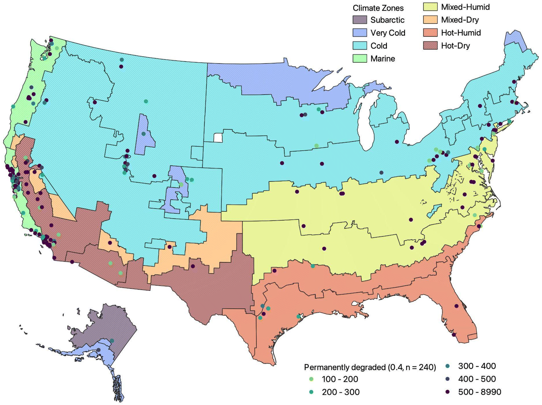 | ||
| Fig. 4 Map of permanently degraded PurpleAir sensors with at least 100 measurements for which the cumulative mean of the flagged indicator ≥ 0.4. The number of hours of operation for which the cumulative mean of the flag indicator is ≥ 0.4 is indicated by point color. | ||
A limitation of using the percentage of flagged measurements as a degradation metric is that it does not account for the possibility that channels A and B might both degrade in a similar manner. Therefore, we rely on a second approach, using collocated reference monitoring measurements, to evaluate this aspect of possible degradation.
463156 measurements (Table S2†). We then used the following eqn (1), as proposed in Barkjohn et al. (2021),33 to correct the PurpleAir sensors with the corresponding reference measurement:| PM2.5, reference = PM2.5 × s1 + RH × s2 + b + ε | (1) |
Here, PM2.5,reference is the reference monitor measurement; PM2.5 is the PurpleAir measurement calculated by averaging concentrations reported by channels A and B; RH is the relative humidity reported by the PurpleAir sensor. We empirically derived coefficients: s1, s2, and b by regressing uncorrected PurpleAir PM2.5 measurements on reference measurements of PM2.5. ε denotes error from a standard normal distribution. We evaluated one correction model for all PurpleAir sensors in our dataset in a similar manner to Barkjohn et al. (2021). We evaluated and plotted the correction error, which is defined as the difference between the corrected measurement and the corresponding reference PM2.5 measurement in μg m−3. In supplementary analyses, we repeat this process using nine additional correction functions ranging from simple linear regressions to more complex machine learning algorithms, some of which additionally correct for T and D, in addition to RH (Table S3†), to evaluate the sensitivity of our results to the correction model used. A key concern is that some part of the correction error observed might not be due to degradation but to inadequate correction of RH or other environmental parameters. We plot correction error versus RH to visually assess if such a dependence exists. Some of the supplementary correction models used to rely on non-linear corrections for RH. Research has shown that a non-linear correction equation might be more suitable to correct for PurpleAir measurements above ∼500 μg m−3 of PM2.5 levels.37 The machine learning models that we used in the supplement can identify such patterns using statistical learning. A full description of these additional models can be found in deSouza et al. (2022).25
2.5 Evaluating associations between the degradation outcomes and time
We evaluated the association between the degradation outcomes under consideration on time of operation using a simple linear regression (Fig. 5):| Degradation outcome = f + d × hour of operation + ε | (2) |
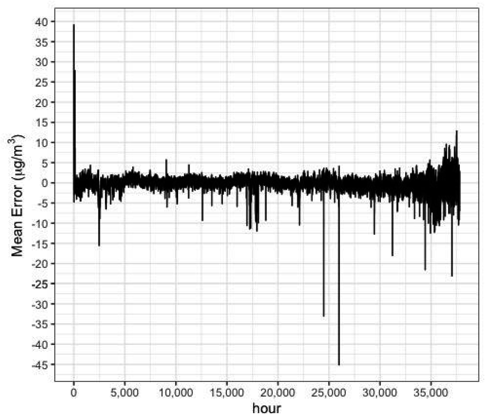 | ||
| Fig. 5 Mean error (μg m−3) calculated as the difference between the corrected PM2.5 measurements from the PurpleAir sensors and the corresponding reference PM2.5 measurements across all sensors as a function of hour of operation. | ||
where f denotes a constant intercept; d denotes the association between operational time (number of hours since each sensor was deployed) and the degradation outcome as the percentage of (cumulative) flagged measurements over all PurpleAir sensors at a given operational time; and ε denotes error from a standard normal distribution.
For the degradation outcomes under consideration, we evaluated whether the associations were different in subgroups stratified by IECC Climate Zones that represent different T and RH conditions (Table S2† contains information on the number of PurpleAir measurements and reported PM2.5 concentrations by climate zone.) When evaluating the impact of climate zone on the percentage of flagged measurements, we examined the impact on outside devices alone, as indoor environments may not always reflect outside conditions due to heating, cooling, general sheltering, etc. Note that when joining climate zones with the complete dataset of PurpleAir IDs, there were a handful of sensors which did not fall within a climate zone. (This was not the case for our subset of collocated PurpleAir sensors.) We removed data corresponding to these sensors when evaluating climate zone-specific associations, corresponding to 2.9% of all data records Fig. S2 in the ESI† shows where these sensors were located.
We also tested whether the cumulative number of PM2.5 measurements recorded over 50, 100, and 500 μg m−3 by individual PurpleAir sensors significantly modifies the association between operational time and the correction error, as previous work has found that low-cost optical PM sensors can degrade after exposure to high PM concentrations.28 As the correction error will be larger at higher PM2.5 concentrations,25,38 we also evaluated this association after normalizing the correction error by (PM2.5,corrected + PM2.5,reference)/2 to make it easier to interpret how cumulative exposure to high PM2.5 measurements can affect the association between degradation and hour of operation.
The merged PurpleAir and reference measurements dataset only included measurements from outdoor PurpleAir sensors. We also evaluated the indoor/outdoor-specific associations between the percentage of flagged measurements and hours of operation.
Finally, we tested for potential non-linearities between the degradation outcomes under consideration and the time of operation. Penalized splines (p-splines) were used to flexibly model the associations between the error and time of operation using a generalized additive model [GAM; degradation outcome ∼s(hour)]. We used a generalized cross-validation (GCV) criterion to select the optimal number of degrees of freedom (df) and plotted the relationships observed. Ninety-five percent confidence intervals (CIs) were evaluated by m-out-n bootstrap, which creates non-parametric CIs by randomly resampling the data. Briefly, we selected a bootstrapped sample of monitors, performed the correction, and then fit GAMs in each bootstrap sample using sensor ID clusters (100 replicates; Fig. 6).
 | ||
| Fig. 6 Response plot and 95% confidence intervals (shaded region) for the association between the degradation outcomes of (A) percentage (%) of flagged measurements and (B) correction error with respect to operational time in hours generated using GAMs. | ||
All analyses were conducted using the software R. In all analyses, p-values <0.05 were taken to represent statistical significance.
3 Results
3.1 Defining a ‘flagged’ PurpleAir measurement
Fig. 2a and b display agreement between the unflagged hourly PurpleAir measurements and the corresponding regulatory measurements using the R and nRMSE metrics, for different percentile thresholds to define a ‘flag’. The lowest nRMSE and highest R were observed for the following definition of a flagged PurpleAir measurement: the absolute difference between PM2.5 from channels A and B > 5 μg m−3 and the % difference between channels A and B: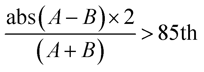 percentile of the percentage difference between channels A and B for each PurpleAir sensor. The 85th percentile of the percentage difference between channels A and B of each PurpleAir varies, with a mean of 38%. This definition resulted in about ∼2% of the PurpleAir data being flagged (Fig. 2c).
When we repeated this analysis excluding measurements from reference monitors that relied on light scattering techniques, using the 86th percentile yielded marginally better results (the metrics differed by < 1%) than using the 85th percentile (Fig. S3 in the ESI†). Given the small difference in results, the 85th percentile is used as the threshold in this study to define a flagged PurpleAir measurement.
3.2 Visualizing the degradation outcomes: percentage of flagged measurements over time
Using the empirically derived definition of flagged measurements, the percentage of flagged measurements, as well as the percentage of cumulative flagged measurements across the 11932 PurpleAir sensors for every hour of operation, is plotted in Fig. 3. The total number of measurements made at every hour of operation is also displayed using the right axis. The percentage of flagged measurements increases over time. At 4 years (∼35000 hours) of operation, the percentage of flagged measurements every hour is ∼4%. After 4 years of operation, we observe a steep increase in the average percentage of flagged measurements, likely due at least in part to the small number of PurpleAir sensors operational for such long periods of time in our dataset. Note that as we rely on a crowd-sourced dataset of PurpleAir measurements, we do not have information on why users removed sensors from operation. Users might have removed PurpleAir sensors that displayed indications of degradation. The removal of such sensors would bias our results, leading to us reporting lower degradation rates than appropriate. We also observe a high percentage of flagged measurements during the first 20 hours of the operation of all sensors.
Using t-tests, we find that the mean of PM2.5, T, and RH measurements were statistically different (p < 0.05) for flagged PurpleAir measurements compared to unflagged measurements (Table 2). PM2.5 and T measurements recorded when a measurement was flagged were higher than for unflagged measurements, whereas RH tended to be lower. The differences between RH and T values for flagged versus non-flagged measurements are small. The difference in PM2.5 distribution was due in part to the way flags have been defined. As data are flagged only if concentrations differ by at least 5 μg m−3 different, the minimum average flagged concentration is 2.5 μg m−3 (e.g., A = 0, B = 5). There are no notable differences between the percentage of flagged measurements made every month.
We next evaluated the number of PurpleAir measurements that were permanently degraded, or that had a cumulative mean of flags over subsequent hours of operation ≥ 0.4 for at least 100 hours of operation (i.e., at least 40% of measurements flagged) (Fig. 4). Table 3 displays the fraction of permanently degraded sensors in different climate zones and different locations (inside/outside). It appears that the largest fraction of degraded sensors occurred in the south-east United States, a hot and humid climate. Fig. S4† displays the cumulative mean of flag for each ‘permanently degraded’ sensor (the title of each plot corresponds to the sensor ID as provided on the PurpleAir website) at each instance of time. Fig. S4† also depicts the starting year of each permanently degraded sensor. The sensor age varied widely over the set of permanently degraded sensors, indicating that permanent degradation is not dictated by time dependence.
| Percentage of permanently degraded sensors | |
|---|---|
| All | 240 out of 11932 (2.0%) |
| Device location | |
| Inside | 2 out of 935 (0.21%) |
| Outside | 238 out of 10997 (2.2%) |
| Climate zone | |
| Cold | 51 out of 2458 (2.1%) |
| Hot-dry | 54 out of 2680 (2.0%) |
| Hot-humid | 11 out of 281 (3.9%) |
| Marine | 84 out of 4842 (1.7%) |
| Mixed-dry | 3 out of 361 (0.8%) |
| Mixed-humid | 24 out of 750 (3.2%) |
| Subarctic | 1 out of 58 (1.7%) |
| Very cold | 3 of 108 (2.8%) |
| No information | 9 of 394 (2.3%) |
Note that from Fig. S4† some of the 240 sensors identified appear to recover or behave normally after a long interval (>100 hours) of degradation (cumulative mean of flag decreases). This could be an artifact of the way the cumulative mean of the flagged indicator is calculated. If the final few measurements of the sensor are not flagged, then the cumulative mean for the final hours of operation of the PurpleAir sensors might be low. It is also possible that some of the sensors could have been temporarily impacted by dust or insects. The owner of the PurpleAir sensors might have cleaned the instruments or replaced the internal Plantower sensors or cleaned out the sensors which could have caused the sensors to recover.
Fig. S5A and S5B† are maps showing locations of PurpleAir sensors that had a cumulative mean of ‘flag’ over subsequent hours of operation of ≥ 0.3 (number of sensors = 323) and 0.5 (number of sensors = 182), respectively, for at least 100 hours of operation.
3.3 Visualization of the error in the corrected PurpleAir PM2.5 measurements over time
The correction derived using a regression analysis yielded the following function to derive corrected PM2.5 concentrations from the raw PurpleAir data: PM2.5,corrected = 5.92 + 0.57PM2.5,raw −0.091RH. After correction, the Pearson correlation coefficient (R) improved slightly, from 0.88 to 0.89, whereas the RMSE improved significantly, from 12.5 to 6.6 μg m−3. The mean, median, and maximum errors observed were 3.3, 2.2, and 792.3 μg m−3, respectively (Table S3†). Fig. 5 displays the mean correction error across all sensors for every hour in operation. The mean error past 35000 hours (3 years) becomes larger, reaching −0.45 μg m−3, compared to −0.13 μg m−3 before. A plot of correction error versus RH did not reveal any associations between the two variables Fig. S6.† We note that similar time dependence of the correction errors was observed when using a wide array of correction models, including models that contain both RH and T as variables, as well as more complex machine learning models that yielded the best correction results (Random Forest: R = 0.99, RMSE = 2.4 μg m−3) (Table S3†).
3.4 Associations between degradation outcomes and operational times
We assessed the association between degradation outcomes and operational time based on eqn (2). We observed that the percentage of flagged measurements increased on average by 0.93% (95% CI: 0.91%, 0.94%) for every year of operation of a PurpleAir sensor. Device location and climate zone were significant effect modifiers of the impact of time-of-operation on this degradation outcome. PurpleAir sensors located outside had an increased percentage of flagged measurements every year corresponding to 1.06% (95% CI 1.05%, 1.08%), whereas those located inside saw the percentage of flagged measurements decrease over time. Outdoor PurpleAir sensors in hot-dry climates appeared to degrade the fastest with the percentage of flagged measurements increasing by 2.09% (95% CI 2.07%, 2.12%) every year in this climate zone (Table 3). Hot-dry places are dustier. Dust can degrade fan performance and accumulate in the air-flow path and optical components which would lead to potentially more disagreement between channels A and B of the PurpleAir sensors.The correction error (PM2.5,corrected–PM2.5,reference) appeared to become negatively biased over time: −0.12 (95% CI −0.13, −0.10) μg m−3 per year of operation, except for sensors in hot and dry environments where the error was positively biased and increased over time by 0.08 (95% CI: 0.06, 0.09) μg m−3 per year of operation. Wildfires often occur in hot-dry environments. Research has shown that the correction approach could overcorrect the PurpleAir measurements at very high smoke concentrations, potentially explaining the disagreement between the corrected PurpleAir and reference measurements in these environments.39 We note that mean PM2.5 concentrations were highest in hot-dry environments (Table S2†). In addition, the number of PM2.5 concentrations >100 μg m−3 recorded was the highest in hot-dry environments. The magnitude of the correction error bias over time appears to be highest in hot and humid environments corresponding to −0.92 (95% CI −1.10, −0.75) μg m−3 per year. RH has an impact on PurpleAir performance and can also cause the electronic components inside the sensors to degrade quickly, so it is not altogether surprising that degradation appears to be highest in hot and humid environments. We observed similar results when regressing the correction errors derived using other correction model forms (Table S4†). Climate zone is a significant modifier of the association between both degradation outcomes and time (Table 4).
| Associations (95% confidence interval) | ||
|---|---|---|
| Dataset | Percentage of flagged measurements | Correction error |
| a (*p < 0.05). | ||
| All | 0.93* (0.91, 0.94) | −0.12* (−0.13, −0.10) |
| Device location | ||
| Inside | −0.10* (−0.12, −0.09) | — |
| Outside | 1.06* (1.05, 1.08) | — |
| Climate zone (outside devices only) | ||
| Cold | 0.74* (0.71, 0.76) | −0.27* (−0.29, −0.25) |
| Hot-dry | 2.09* (2.07, 2.12) | 0.08* (0.06, 0.09) |
| Hot-humid | 0.34* (0.32, 0.37) | −0.92* (−1.10, −0.75) |
| Marine | 0.41* (0.39, 0.44) | −0.13* (−0.15, −0.10) |
| Mixed-dry | −0.05* (−0.07, −0.02) | −0.31* (−0.40, −0.21) |
| Mixed-humid | 0.54* (0.51, 0.57) | −0.28* (−0.33, −0.23) |
| Sub arctic | −0.18* (−0.22, −0.14) | — |
| Very cold | 0.13* (0.10, 0.16) | — |
The cumulative number of PM2.5 measurements recorded over 50, 100, and 500 μg m−3 modifies the association between operational time and the correction error significantly, in the negative direction (Table S5†), meaning that sensors that experience more high concentration episodes are more likely to underestimate PM2.5. The increase in the negative bias of the corrected sensor data could be because the absolute magnitude of the correction error will be higher in high PM2.5 environments. When we evaluated the impact of the cumulative number of high PM2.5 measurements on the association between the normalized correction error and operation hour (hours since deployment), we found that the cumulative number of high PM2.5 measurements was not a significant effect modifier of this association (Table S6†). In other words, we did not observe sensors in higher PM2.5 environments degrading faster.
3.5 Evaluating potential non-linearities between the degradation outcomes and time
GCV criteria revealed that the dependence of the percentage of flagged PurpleAir measurements over time was non-linear, likely due to the non-linear relationship observed at operational times greater than 30000 hours (3.5 years; Fig. 6). However, due to the small number of measurements after this time interval, the shape of the curve after this time was uncertain, as evidenced by the wide confidence bands in this time period. The correction error appeared to become more and more negatively biased after 30000 operational hours (3.5) years. However, due to the small number of sensors operating for more than 3 years, the wide confidence interval bands past 3 years cast uncertainty on the latter finding. A possible reason we see an increase in correction error is because of wildfire smoke in the summer of 2020 that potentially affected sensors deployed in January 2017. However, the wide range of start month-year of sensors >3.5 years in our dataset suggests that this is unlikely.
4 Discussion and conclusions
We evaluated two proposed degradation outcomes for the PurpleAir sensors over time. We observed there were a large number of measurements from channels A and B of each sensor during the first 20 hours of operation that were flagged (Fig. 1). Some of these data might come from laboratory testing of the PurpleAir sensors. Our results suggest that it is important to delete the first 20 hours of data when analyzing PurpleAir measurements. We observed that the percentage of flagged measurements (where channels A and B diverged) increased linearly over time and was on average ∼4% after 3 years of operation. It appears that measurements from PurpleAir sensors are fairly robust, at least during this period. Degradation appears to increase steeply after 4 years from 5% to 10% in just 6 months. It thus appears that PurpleAir sensors might need to be serviced or the Plantower sensors replaced after ∼4 years of operation. However, given the small number of Plantower devices operational after 4 years (<100), further work is needed to evaluate the performance of devices aged 4 years or more. We also note that although many low-cost sensors use Plantower sensors, just like the PurpleAir sensors our analysis may not be generalizable to these devices if they have outer shells that can offer potentially more protection than the PurpleAir, or if there are other design differences that might affect instrument performance.Flagged measurements were more likely to be observed at higher PM2.5 concentrations, lower RH levels, and higher T levels (Table 1). When we evaluated associations between the percentage of flagged measurements and year of operation for sensors in different locations (i.e., outdoor vs. indoor), we found that outdoor sensors degrade much faster than indoor sensors (Table 3). As T and RH impact the likelihood of observing a flagged measurement, this could be because environmental conditions of indoor environments (T and RH) are more regulated than outdoor environments, and indoor instruments tend to be more protected. Our results indicate that the percentage of flagged measurements for indoor environments decreases over time. This could be because of the high percentage of flagged measurements observed in the first 20 hours of operation, and the lack of large changes in the percentage of flagged measurements in later hours of operation in comparison to outdoor sensors. We also note that there is a much smaller number of indoor sensors compared to outdoor instruments (935 compared to 10997), and thus far fewer measurements available, especially at long operational time intervals.
For outdoor sensors, we found that the climate zone in which the sensor was deployed is an important modifier of the association between the percentage of flagged measurements and time. Outdoor sensors in hot-dry climates degrade the fastest, with the percentage of flagged measurements increasing by 2.09% (95% CI 2.07%, 2.12%) every year, an order of magnitude faster than any other climate zone (Table 3). This suggests that on average, outdoor sensors in hot-dry climates likely need to be serviced after ∼3 years, faster than PurpleAir sensors deployed elsewhere.
There was a small number of PurpleAir sensors (240 out of 11932) that were permanently degraded (the cumulative mean of subsequent measurements had over 40% degraded measurements for at least 100 hours). The list of permanently degraded PurpleAir IDs is presented in Fig. S4.† These sensors should be excluded when conducting analyses. The largest fraction of permanently degraded PurpleAir sensors appeared to be in the hot and humid climate zone indicating that sensors in these climates likely needed to be replaced sooner than in others (Table 2). There was no significant relationship between sensor age and permanent degradation, indicating that there may be other factors responsible for causing permanent failure among the PurpleAir sensors. For example, anecdotal evidence suggests that the PurpleAir sensors can be impacted by dust or even insects and degrade the internal components of one or the other PurpleAir channels.
When evaluating the time dependence of the correction error, we found that the PurpleAir instrument bias changes by −0.12 (95% CI: −0.13, −0.10) μg m−3 per year of operation. However, the low associations indicate that this bias is not of much consequence to the operation of PurpleAir sensors. Climate zone was a significant effect modifier of the association between bias and time. The highest associations were observed in hot and humid regions corresponding to −0.92 (95% CI −1.10, −0.75) μg m−3 per year. Exposure to a cumulative number of high PM2.5 measurements did not significantly affect the association between the normalized correction error over time.
It is not altogether surprising that the correction error increases most rapidly in hot and humid climate zones, as past evidence suggests that the performance of PurpleAir is greatly impacted by RH. It is surprising that this is not the case for the other degradation outcomes considered in this study: % of flagged measurements. It is likely that the percentage of flagged measurements increases most rapidly over time in hot and dry environments because such environments tend to be dusty and dust can degrade fan performance and accumulate in the air flow path and optical components of the PurpleAir sensors which can lead to disagreement between the two Plantower sensors. We note that under conditions of wildfire smoke, also prevalent in hot and dry climates, the calibration error could also be magnified due to under-correction of the PurpleAir data. Future work is needed to evaluate the impact of wildfire-smoke on the performance of PurpleAir sensors.
When accounting for non-linearities in the relationship between the correction error and time, Fig. 6a indicates that the bias in the correction error is not linear with time; rather it increases significantly after 30000 hours or 3.5 years. Overall, we found that more work is needed to evaluate degradation in PurpleAir sensors after 3.5 years of operation, due to a paucity of longer-running sensors in the database. Importantly, the degradation outcomes derived in this paper can be used to remove ‘degraded’ PurpleAir measurements in other analyses. We also show that concerns about degradation are more important in some climate zones than others, which may necessitate appropriate cleaning or other maintenance procedures for sensors in different locations.
Disclaimer
The views expressed in this paper are those of the author(s) and do not necessarily represent the views or policies of the US Environmental Protection Agency. Any mention of trade names, products, or services does not imply an endorsement by the US Government or the US Environmental Protection Agency. The EPA does not endorse any commercial products, services, or enterprises.Conflicts of interest
There are no conflicts to declare.Acknowledgements
The authors are grateful to Mike Bergin and John Volckens for several useful discussions. Thanks to PurpleAir (https://www2.purpleair.com/) for providing publicly the data that made this paper possible.References
- P. deSouza, D. Braun, R. M. Parks, J. Schwartz, F. Dominici and M.-A. Kioumourtzoglou, Nationwide Study of Short-Term Exposure to Fine Particulate Matter and Cardiovascular Hospitalizations Among Medicaid Enrollees, Epidemiology, 2020, 32(1), 6–13, DOI:10.1097/EDE.0000000000001265.
- P. N. deSouza, M. Hammer, P. Anthamatten, P. L. Kinney, R. Kim, S. V. Subramanian, M. L. Bell and K. M. Mwenda, Impact of Air Pollution on Stunting among Children in Africa, Environ. Health, 2022, 21(1), 128, DOI:10.1186/s12940-022-00943-y.
- P. N. deSouza, S. Dey, K. M. Mwenda, R. Kim, S. V. Subramanian and P. L. Kinney, Robust Relationship between Ambient Air Pollution and Infant Mortality in India, Sci. Total Environ., 2022, 815, 152755, DOI:10.1016/j.scitotenv.2021.152755.
- A. F. Boing, P. deSouza, A. C. Boing, R. Kim and S. V. Subramanian, Air Pollution, Socioeconomic Status, and Age-Specific Mortality Risk in the United States, JAMA Netw. Open, 2022, 5(5), e2213540, DOI:10.1001/jamanetworkopen.2022.13540.
- P. deSouza, A. F. Boing, R. Kim and S. Subramanian, Associations between Ambient PM2.5 – Components and Age-Specific Mortality Risk in the United States, Environ. Adv., 2022, 9, 100289, DOI:10.1016/j.envadv.2022.100289.
- H. E. Institute. State of Global Air 2019. Health Effects Institute Boston, MA, 2019 Search PubMed.
- K.-H. Kim, E. Kabir and S. Kabir, A Review on the Human Health Impact of Airborne Particulate Matter, Environ. Int., 2015, 74, 136–143, DOI:10.1016/j.envint.2014.10.005.
- H. L. Brantley, G. S. W. Hagler, S. C. Herndon, P. Massoli, M. H. Bergin and A. G. Russell, Characterization of Spatial Air Pollution Patterns Near a Large Railyard Area in Atlanta, Georgia, Int. J. Environ. Res. Public Health, 2019, 16(4), 535, DOI:10.3390/ijerph16040535.
- P. deSouza, A. Anjomshoaa, F. Duarte, R. Kahn, P. Kumar and C. Ratti, Air Quality Monitoring Using Mobile Low-Cost Sensors Mounted on Trash-Trucks: Methods Development and Lessons Learned, Sustain. Cities Soc., 2020, 60, 102239, DOI:10.1016/j.scs.2020.102239.
- P. deSouza. A. Wang. Y. Machida. T. Duhl. S. Mora. P. Kumar. R. Kahn. C. Ratti. J. L. Durant and N. Hudda. Evaluating the Performance of Low-Cost PM2.5 Sensors in Mobile Settings. arXiv January 10, 2023, preprint, 10.48550/arXiv.2301.03847.
- P. deSouza, R. Lu, P. Kinney and S. Zheng, Exposures to Multiple Air Pollutants While Commuting: Evidence from Zhengzhou, China, Atmos. Environ., 2020, 118168, DOI:10.1016/j.atmosenv.2020.118168.
- P. N. deSouza, P. A. Oriama, P. P. Pedersen, S. Horstmann, L. Gordillo-Dagallier, C. N. Christensen, C. O. Franck, R. Ayah, R. A. Kahn, J. M. Klopp, K. P. Messier and P. L. Kinney, Spatial Variation of Fine Particulate Matter Levels in Nairobi before and during the COVID-19 Curfew: Implications for Environmental Justice, Environ. Res. Commun., 2021, 3(7), 071003, DOI:10.1088/2515-7620/ac1214.
- P. deSouza and P. L. Kinney, On the Distribution of Low-Cost PM 2.5 Sensors in the US: Demographic and Air Quality Associations, J. Exposure Sci. Environ. Epidemiol., 2021, 31(3), 514–524, DOI:10.1038/s41370-021-00328-2.
- G. Anderson and R. Peng, Weathermetrics: Functions to Convert between Weather Metrics (R Package), 2012 Search PubMed.
- R. Williams, V. Kilaru, E. Snyder, A. Kaufman, T. Dye, A. Rutter, A. Russel and H. Hafner, Air Sensor Guidebook, US Environmental Protection Agency, Washington, DC, EPA/600/R-14/159 NTIS PB2015-100610, 2014 Search PubMed.
- N. Castell, F. R. Dauge, P. Schneider, M. Vogt, U. Lerner, B. Fishbain, D. Broday and A. Bartonova, Can Commercial Low-Cost Sensor Platforms Contribute to Air Quality Monitoring and Exposure Estimates?, Environ. Int., 2017, 99, 293–302, DOI:10.1016/j.envint.2016.12.007.
- P. Kumar, L. Morawska, C. Martani, G. Biskos, M. Neophytou, S. Di Sabatino, M. Bell, L. Norford and R. Britter, The Rise of Low-Cost Sensing for Managing Air Pollution in Cities, Environ. Int., 2015, 75, 199–205, DOI:10.1016/j.envint.2014.11.019.
- L. Morawska, P. K. Thai, X. Liu, A. Asumadu-Sakyi, G. Ayoko, A. Bartonova, A. Bedini, F. Chai, B. Christensen, M. Dunbabin, J. Gao, G. S. W. Hagler, R. Jayaratne, P. Kumar, A. K. H. Lau, P. K. K. Louie, M. Mazaheri, Z. Ning, N. Motta, B. Mullins, M. M. Rahman, Z. Ristovski, M. Shafiei, D. Tjondronegoro, D. Westerdahl and R. Williams, Applications of Low-Cost Sensing Technologies for Air Quality Monitoring and Exposure Assessment: How Far Have They Gone?, Environ. Int., 2018, 116, 286–299, DOI:10.1016/j.envint.2018.04.018.
- E. G. Snyder, T. H. Watkins, P. A. Solomon, E. D. Thoma, R. W. Williams, G. S. W. Hagler, D. Shelow, D. A. Hindin, V. J. Kilaru and P. W. Preuss, The Changing Paradigm of Air Pollution Monitoring, Environ. Sci. Technol., 2013, 47(20), 11369–11377, DOI:10.1021/es4022602.
- P. N. deSouza, Key Concerns and Drivers of Low-Cost Air Quality Sensor Use, Sustainability, 2022, 14(1), 584, DOI:10.3390/su14010584.
- P. deSouza, V. Nthusi, J. M. Klopp, B. E. Shaw, W. O. Ho, J. Saffell, R. Jones and C. Ratti, A Nairobi Experiment in Using Low Cost Air Quality Monitors, Clean Air J., 2017, 27(2), 12–42 Search PubMed.
- T. Lu, M. J. Bechle, Y. Wan, A. A. Presto and S. Hankey, Using Crowd-Sourced Low-Cost Sensors in a Land Use Regression of PM2.5 in 6 US Cities, Air Qual., Atmos. Health, 2022, 15(4), 667–678, DOI:10.1007/s11869-022-01162-7.
- J. Bi, A. Wildani, H. H. Chang and Y. Liu, Incorporating Low-Cost Sensor Measurements into High-Resolution PM2.5 Modeling at a Large Spatial Scale, Environ. Sci. Technol., 2020, 54(4), 2152–2162, DOI:10.1021/acs.est.9b06046.
- P. deSouza, R. A. Kahn, J. A. Limbacher, E. A. Marais, F. Duarte and C. Ratti, Combining Low-Cost, Surface-Based Aerosol Monitors with Size-Resolved Satellite Data for Air Quality Applications, Atmos. Meas. Tech. Discuss., 2020, 1–30, DOI:10.5194/amt-2020-136.
- P. deSouza, R. Kahn, T. Stockman, W. Obermann, B. Crawford, A. Wang, J. Crooks, J. Li and P. Kinney, Calibrating Networks of Low-Cost Air Quality Sensors, Atmos. Meas. Tech. Discuss., 2022, 1–34, DOI:10.5194/amt-2022-65.
- M. R. Giordano, C. Malings, S. N. Pandis, A. A. Presto, V. F. McNeill, D. M. Westervelt, M. Beekmann and R. Subramanian, From Low-Cost Sensors to High-Quality Data: A Summary of Challenges and Best Practices for Effectively Calibrating Low-Cost Particulate Matter Mass Sensors, J. Aerosol Sci., 2021, 158, 105833, DOI:10.1016/j.jaerosci.2021.105833.
- C. Malings, D. M. Westervelt, A. Hauryliuk, A. A. Presto, A. Grieshop, A. Bittner, M. Beekmann and R. Subramanian, Application of Low-Cost Fine Particulate Mass Monitors to Convert Satellite Aerosol Optical Depth to Surface Concentrations in North America and Africa, Atmos. Meas. Tech., 2020, 13, 3873–3892, DOI:10.5194/amt-13-3873-2020.
- J. Tryner, J. Mehaffy, D. Miller-Lionberg and J. Volckens, Effects of Aerosol Type and Simulated Aging on Performance of Low-Cost PM Sensors, J. Aerosol Sci., 2020, 150, 105654, DOI:10.1016/j.jaerosci.2020.105654.
- L. Sun, D. Westerdahl and Z. Ning, Development and Evaluation of A Novel and Cost-Effective Approach for Low-Cost NO2 Sensor Drift Correction, Sensors, 2017, 17(8), 1916, DOI:10.3390/s17081916.
- G. Tancev, Relevance of Drift Components and Unit-to-Unit Variability in the Predictive Maintenance of Low-Cost Electrochemical Sensor Systems in Air Quality Monitoring, Sensors, 2021, 21(9), 3298, DOI:10.3390/s21093298.
- K. Ardon-Dryer, Y. Dryer, J. N. Williams and N. Moghimi, Measurements of PM2.5 with PurpleAir under Atmospheric Conditions, Atmos. Meas. Tech. Discuss., 2019, 1–33, DOI:10.5194/amt-2019-396.
- K. E. Kelly, J. Whitaker, A. Petty, C. Widmer, A. Dybwad, D. Sleeth, R. Martin and A. Butterfield, Ambient and Laboratory Evaluation of a Low-Cost Particulate Matter Sensor, Environ. Pollut., 2017, 221, 491–500, DOI:10.1016/j.envpol.2016.12.039.
- K. K. Barkjohn, B. Gantt and A. L. Clements, Development and Application of a United States-Wide Correction for PM2.5 Data Collected with the PurpleAir Sensor, Atmos. Meas. Tech., 2021, 14(6), 4617–4637, DOI:10.5194/amt-14-4617-2021.
- T. Sayahi, D. Kaufman, T. Becnel, K. Kaur, A. E. Butterfield, S. Collingwood, Y. Zhang, P.-E. Gaillardon and K. E. Kelly, Development of a Calibration Chamber to Evaluate the Performance of Low-Cost Particulate Matter Sensors, Environ. Pollut., 2019, 255, 113131, DOI:10.1016/j.envpol.2019.113131.
- G. Hagler, T. Hanley, B. Hassett-Sipple, R. Vanderpool, M. Smith, J. Wilbur, T. Wilbur, T. Oliver, D. Shand, V. Vidacek, C. Johnson, R. Allen and C. D'Angelo, Evaluation of Two Collocated Federal Equivalent Method PM2.5 Instruments over a Wide Range of Concentrations in Sarajevo, Bosnia and Herzegovina, Atmos. Pollut. Res., 2022, 13(4), 101374, DOI:10.1016/j.apr.2022.101374.
- M. Kushwaha, V. Sreekanth, A. R. Upadhya, P. Agrawal, J. S. Apte and J. D. Marshall, Bias in PM2.5 Measurements Using Collocated Reference-Grade and Optical Instruments, Environ. Monit. Assess., 2022, 194(9), 610, DOI:10.1007/s10661-022-10293-4.
- L. Wallace, J. Bi, W. R. Ott, J. Sarnat and Y. Liu, Calibration of Low-Cost PurpleAir Outdoor Monitors Using an Improved Method of Calculating PM2.5, Atmos. Environ., 2021, 256, 118432, DOI:10.1016/j.atmosenv.2021.118432.
- E. M. Considine, D. Braun, L. Kamareddine, R. C. Nethery and P. deSouza, Investigating Use of Low-Cost Sensors to Increase Accuracy and Equity of Real-Time Air Quality Information, Environ. Sci. Technol., 2023 DOI:10.1021/acs.est.2c06626.
- K. K. Barkjohn, A. L. Holder, S. G. Frederick and A. L. Clements, Correction and Accuracy of PurpleAir PM2.5 Measurements for Extreme Wildfire Smoke, Sensors, 2022, 22(24), 9669, DOI:10.3390/s22249669.
Footnote |
| † Electronic supplementary information (ESI) available. See DOI: https://doi.org/10.1039/d2ea00142j |
| This journal is © The Royal Society of Chemistry 2023 |