
 Open Access Article
 This Open Access Article is licensed under a
 Creative Commons Attribution 3.0 Unported Licence
Development of volatility distributions for organic matter in biomass burning emissions†
Aditya
Sinha
a,
Ingrid
George
b,
Amara
Holder
b,
William
Preston
c,
Michael
Hays
 b and
Andrew P.
Grieshop
*a
b and
Andrew P.
Grieshop
*a
aDepartment of Civil and Environmental Engineering, North Carolina State University, Raleigh, NC, USA. E-mail: apgriesh@ncsu.edu
bCenter for Environmental Measurement and Modeling, US Environmental Protection Agency, Durham, NC, USA
cCSS Inc., Durham, NC, USA
First published on 7th October 2022
Abstract
The volatility distribution of organic emissions from biomass burning and other combustion sources can determine their atmospheric evolution due to partitioning/aging. The gap between measurements and models predicting secondary organic aerosol has been partially attributed to the absence of semi- and intermediate volatility organic compounds (S/I-VOC) in models and measurements. However, S/I-VOCs emitted from these sources and typically quantified using the volatility basis framework (VBS) are not well understood. For example, the amount and composition of S/I-VOCs and their variability across different biomass burning sources such as residential woodstoves, open field burns, and laboratory simulated open burning are uncertain. To address this, a novel filter-in-tube sorbent tube sampling method collected S/I-VOC samples from biomass burning experiments for a range of fuels and combustion conditions. Filter-in-tube samples were analyzed using thermal desorption-gas chromatography-mass spectrometry (TD/GC/MS) for compounds across a wide range of volatilities (saturation concentrations; −2 ≤ log![[thin space (1/6-em)]](https://www.rsc.org/images/entities/char_2009.gif) C* ≤ 6). The S/I-VOC measurements were used to calculate volatility distributions for each emission source. The distributions were broadly consistent across the sources with IVOCs accounting for 75–90% of the total captured organic matter, while SVOCs and LVOCs were responsible for 6–13% and 1–12%, respectively. The distributions and predicted partitioning were generally consistent with the literature. Particulate matter emission factors spanned two orders of magnitude across the sources. This work highlights the potential of inferring gas–particle partitioning behavior of biomass burning emissions using filter-in-tube sorbent samples analyzed offline. This simplifies both sampling and analysis of S/I-VOCs for studies focused on capturing the full range of organics emitted.
C* ≤ 6). The S/I-VOC measurements were used to calculate volatility distributions for each emission source. The distributions were broadly consistent across the sources with IVOCs accounting for 75–90% of the total captured organic matter, while SVOCs and LVOCs were responsible for 6–13% and 1–12%, respectively. The distributions and predicted partitioning were generally consistent with the literature. Particulate matter emission factors spanned two orders of magnitude across the sources. This work highlights the potential of inferring gas–particle partitioning behavior of biomass burning emissions using filter-in-tube sorbent samples analyzed offline. This simplifies both sampling and analysis of S/I-VOCs for studies focused on capturing the full range of organics emitted.
Environmental significanceOrganic emissions from biomass burning are a key contributor to atmospheric composition at all scales. Organic volatility dictates their gas–particle partitioning and contribution to secondary organic aerosol formation. Previous studies have not addressed the volatility of the diverse range of biomass combustion types, largely due to the complexity of quantifying organic volatility. Here, we present results from a novel sampling and analytical approach applied to a range of biomass combustion systems (lab burning of wildland fuels, open grassland burning, residential wood combustion). Our results demonstrate that this relatively simple and field-deployable approach yields volatility distribution that are broadly consistent with previous estimates, but that are distinct between combustion types. While organic PM emission factors ranged over two orders of magnitude across the sources tested, volatility distributions had smaller, though consistent inter-source differences. |
1. Introduction
Emissions from biomass burning significantly influence gas and particle concentrations globally.1 These emissions include major greenhouse gases like carbon dioxide (CO2), air pollutants like carbon monoxide (CO), and volatile organic compounds (VOCs) capable of undergoing photo-oxidation to form secondary products. The products of incomplete combustion from these emissions also include fine particles or particulate matter smaller than 2.5 μm (PM2.5). PM2.5 is an important atmospheric pollutant that has large yet uncertain impacts on climate,1 air quality2 and adversely affects human health.3,4 Modeling studies have shown that residential emissions can make substantial contributions to ambient air pollution (e.g. ∼20−50% of PM2.5 in India).5,6 Further, emission inventories have estimated that 26−73% of global emission of fine particulate organic matter can be ascribed to open biomass burning and about 20% to residential biomass combustion.7–10 This indicates that primary organic aerosol (POA) emitted from biomass burning forms an important component of PM2.5. It is now well understood that biomass burning POA is semi-volatile in nature, i.e., the organic compounds that constitute POA can partition between the gas and particle phases.11–14 This partitioning can vary with atmospheric dilution and ambient temperature, which shift the thermodynamic equilibrium, influencing the fate and lifetime of biomass burning POA. Accounting for gas–particle partitioning in emissions inventories can have important implications for predictions of chemical transport models (CTMs) and enable more accurate depictions of atmospheric aerosols. Gas–particle partitioning also creates inconsistencies in the definitions of particulate organic matter between regulatory measurements and air quality research models/measurements.15,16 However, few studies have made attempts to constrain the partitioning behavior of biomass burning POA.The gas–particle partitioning of POA in the atmosphere is typically described using absorptive partitioning theory.17,18 This theory can be used in a semi-empirical fashion with a set of surrogate or lumped species that describes the measured partitioning behavior of emissions.12,14 This surrogate set of compounds is often represented using a one-dimensional volatility basis set, or VBS,18 which distributes organics over a logarithmically spaced set of bins of effective saturation concentration, Ci*. In this framework, resolution of POA at a molecular level is not required as surrogate bins describe the properties of compounds lumped in the bin (e.g., saturation concentration). At phase equilibrium, the organic aerosol (OA) emission factor (EFOA) and the mass fraction of organic emissions residing in the particle phase (Xp) are expressed as:
 | (1) |
 is the effective saturation concentration of species i at temperature T, COA is the OA concentration, fi is the mass fraction of species i, and EFTOT is the emission factor of all lower-volatility organics (particle and gas phase) being captured.
Organics can be segregated into volatility groups based on the nomenclature proposed elsewhere19,20 as: intermediate volatility organic compounds, IVOCs (C* = 300–3 × 10⁶ μg m−3), semi-volatile organic compounds, SVOCs (C* = 0.3–300 μg m−3) and low volatility organic compounds, LVOCs (C* < 0.3 μg m−3). S/I-VOCs play an important role in describing gas–particle partitioning from biomass burning emissions. S/I-VOCs are also important precursors for secondary organic aerosol (SOA) formation and likely play a key role in reducing the gap between measurements and models predicting SOA formation.13,21 However, quantitative collection and chemical analysis of this material, and especially IVOCs, is complex. For example, in gas chromatography (GC) analysis, the vast majority of IVOCs typically elute in the chromatogram as unresolved complex mixtures (UCM), which is material that co-elutes and cannot be separated into individual compounds.22,23 This is because IVOCs, typically consisting of compounds with carbon numbers greater than 10, are associated with a larger number of constitutional isomers, making them harder to resolve using traditional GC methods. As a result, little research has explored the speciation of S/I-VOCs in both gas and particle phases from biomass burning emissions. Previous studies have sampled from controlled/closed burning and reported gas and particle phase S/I-VOCs for three types of residential wood combustion (RWC)24 and also measured RWC emissions with online methods.25 Other studies have explored emissions from uncontrolled/open burning emissions. For example, one analysis explored emissions from six foliar fuels using ion chromatography and wavelength dispersive X-ray fluorescence techniques.26 Another investigated emissions from a range of fuel types and burning conditions, including laboratory, fireplace, and prescribed fires using electron impact ionization gas chromatography interfaced with mass spectrometry.27 A key commonality of these studies of speciated S/I-VOC compounds is that they typically only identify a fraction (40–50% or less) of the total mass with the remaining fraction apportioned to the UCM. Speciation methods thus have offered detailed chemical information on the identified fraction but have thus far not characterized the UCM (majority contribution in terms of mass). On the other hand, bulk methods (e.g., thermooptical filter measurements of OC) offer little chemical detail but, depending on sampling media, are more likely to capture the full range of mass sampled. Thus, there exists a tradeoff in detailed speciation measurements and measuring the full volatility range of organic mass.
Several methods have been used to estimate volatility distributions of combustion emissions over the last decade. The positive artifact on quartz filters has been used to provide an estimate of gas–particle partitioning.14,28–30 Isothermal dilution and temperature perturbations using thermodenuders have been used to constrain gas–particle partitioning of biomass burning aerosol from wood stoves31 and laboratory fires.11 Several studies have shown that equilibrium cannot be assumed when using thermal denuder systems, thus this tool typically requires application of kinetic equations to estimate volatility distributions.32–34 More recently, a study has estimated volatility distributions of sewage incineration emissions using online mass spectroscopy, capable of measuring low concentrations of gas- and particle phase organics in real-time.35 Another strategy has been the use of thermal desorption gas chromatography mass spectrometry (TD/GC/MS) to infer POA volatility via separation across the retention time in the GC column of organics desorbed from sorbent tubes.22,30,36–39 The volatility distributions derived from TD/GC/MS measurements have been shown to be in agreement with distributions from isothermal dilution/temperature perturbations with kinetic modeling for diesel and gasoline engine emissions.28,30 This method allows for the estimation of organic aerosol volatility from a single sample and thus offers an important advantage over more resource intensive online approaches (e.g., thermodenuders, dilution). However, this method has not been previously used to characterize biomass burning POA volatility. Moreover, a variation of this method with the filter placed inside the sample collection tube allowing for sampling of gas and particle phase organics for simultaneous analysis in the TD/GC/MS has not been attempted for biomass burning emissions. This novel filter-in-tube measurement approach would simplify both sampling and analysis of sorbents for studies focused on capturing the full range of S/I-VOCs emitted.
Biomass burning spans a spectrum ranging from residential wood stoves to open burning resulting in complex mixtures of organic compounds that span a wide range of volatility. Studies have constrained the volatility distributions of biomass burning POA emissions from wood stoves12 and also from laboratory burns of 15 fuels over a range of combustion conditions.11 The recommended distributions derived in May et al.11 have been used in several modeling studies.40–42 Other studies have obtained distributions for open-burning emissions via factor analysis of ambient and thermally denuded OA.43 Another approach was to sample on Solid Phase Extraction (SPE) filters for untargeted analysis of gas-phase S/I-VOCs in biomass burning smoke samples from a series of laboratory fires and subsequently derive volatility distributions from the speciated data.44 However, there is still uncertainty in the amount and composition of S/I-VOCs and how they are influenced by factors like fuel type and combustion conditions. Moreover, quantitative comparison of samples of fresh emissions from lab simulated open burning with those from real-world open burning is lacking. Thus, there is a need to measure partitioning parameters across a broader range of biomass burning conditions and compare them with existing parameterizations.
In this study, we address these knowledge gaps by measuring the volatility distributions from three different types of biomass burning emissions: open field burns, laboratory-simulated open burns and different phases of residential wood combustion in a modern heating stove. S/I-VOC volatility was investigated using a calibration built from n-alkane standards in TD/GC/MS analyses. The objectives of this study are as follows: (1) develop an approach and calibration to map TD/GC/MS data to VBS space; (2) characterize deviations from n-alkane-based calibration in deriving volatility distributions from TD/GC/MS chromatograms; (3) compare volatility distributions from different types of biomass burning using filter-in-tube sorbent samples analyzed using a TD/GC/MS; (4) make comparisons of the derived volatility distributions to existing distributions for biomass burning in literature.
2. Materials and methods
2.1 Experimental setup of combustion experiments
Several different sample types were collected to capture a range of biomass burning conditions, including in-field open burning, laboratory simulations of open burning, and laboratory testing of woodstoves. Sampling times and dilution ratios for the S/I-VOC samples were designed to obtain approximately the same amount of sample mass over the entire duration of each process, while avoiding breakthrough conditions. Breakthrough testing across several emissions testing environments was conducted, including those examining wildfire, residential burning, and vehicle emissions. Breakthrough testing is normally accomplished by positioning two tubes in series and analyzing both using identical GC-MS methodology. At the flow rates, dilution ratios, and concentrations in the present study, compound breakthrough in the second tube has not been observed. In addition, the recovery of the internal standards spiked before sampling was monitored, and the d8-naphthalene internal standard recovery would indicate breakthrough issues during each sampling event.In-field open burning (also referred to as ‘field’): emissions were sampled from three in-field burns of Tallgrass Prairie in the Flint Hills region of Kansas in April 2019. Mobile measurement platforms were positioned immediately downwind of the burning field to capture fresh emissions (Fig. S1-A†). Background air samples were taken on days when no burning occurred. Concurrent measurements of CO, CO2, PM2.5, and elemental (EC) and organic carbon (OC) were made using a portable sampling package described elsewhere.45,46 Briefly, continuous measurements of CO2 were made with a nondispersive infrared analyzer (LiCor, Li-820) and CO with an electrochemical sensor (SGX, EC4-500). Batch samples with Teflon (Teflo, Pall) and quartz (Tissuquartz, Pall) 47 mm filters benhind a PM2.5 impactor inlet were taken simultaneously with a pressure-compensating pump at 10 l min−1 (Leland Legacy, SKC). EC and OC were quantified using the modified NIOSH 5040 protocol described elsewhere.47
Laboratory simulations of open burning (also referred to as ‘burnhut’): fuel was collected from two locations in a conifer forest in northern and central Minnesota. The fuel samples consisted of four clip plots (two 1 m2 and two 0.25 m2) consisting of mostly moss and tree litter and two peat cores taken from the same sites. Open biomass burning was simulated in an open burn test facility (OBTF) on the EPA campus in Research Triangle Park, NC48 (Fig. S1-B†). The OBTF is a 70 m3 room with a high-volume blower that pulls ambient air into the room and out through an exhaust duct (12 inch diameter) to provide excess oxygen conditions. Fuels were dried at 80 °C overnight in an oven before burning. Fuels were evenly dispersed across a 0.5 m2 stainless steel pan filled with sand and covered with aluminum foil and ignited with a propane torch. A nichrome wire was used to ignite the peat cores at one end resulting in smoldering combustion front propagating across the core. Emissions measurements were all taken in the exhaust duct at the same location. Batch samples for PM2.5, EC, OC were collected through a 12 mm OD stainless-steel sample probe and PM2.5 cyclone (URG). An aerosol splitter was used to split the sample between 47 mm Teflon filters (Teflo, Pall) and 90 mm quartz filters (Tissuquartz, Pall). S/I-VOC and black carbon samples were collected through a 6 mm OD stainless-steel sample probe. Continuous measurements of CO, CO2 (CAI, 600 series), NOx (EcoPhysics nCLD), and total hydrocarbons (THC) (CAI, 600 series) were collected through a 6 mm OD stainless-steel probe, heated filter, and heated Teflon sample line.
Laboratory testing of woodstoves (also referred to as ‘RWC’): residential wood combustion (RWC) emissions were sampled from an EPA 2015 certified woodstove (Englander, 30-NC) following a modified cordwood test protocol (ASTM E3053). The method includes a startup phase followed by a high fire phase where the stove air inlets are fully opened and ending with a low fire phase where stove air inlets are fully closed. Tests were done in triplicate for two fuel types: dry Red Oak and dry Sitka Spruce. Fuel wood was cut to nominally 40 cm in length and split into triangular pieces with the bark on (∼0.5–2.5 kg). The test facility is described in detail elsewhere49 and a schematic shown in Fig. S1-C.† Briefly, stove emissions are captured by a hood into an exhaust duct and subsequently mixed with filtered air to reduce temperatures and concentrations. Gas phase emissions (CO2, CO, THC, NOx; CAI 600 series) were sampled through a stainless-steel probe, heated filter, and heated sample line from the dilution duct. PM2.5 (47 mm Telfo, Pall) and EC/OC (47 mm Tissuquartz, Pall) samples were taken from the duct through 6 mm OD stainless steel probes. A secondary dilution system (DI-1000, Dekati) was used to further reduce pollutant concentrations so that SVOC samples could be collected over the entire test phase duration and have concentrations comparable to the field and burnhut samples. SVOC and black carbon (MA350, Aehtlabs) were sampled from a manifold connected to the secondary dilution system. Emissions were sampled from the exhaust duct with a stainless-steel probe (3/8′′) using an eductor (DI-1000, Dekati) supplied with 20 l min−1 of dilution air dried and scrubbed of CO2 (Van Air Compressed Gas Dryer) and supplied to a stainless-steel (Schedule 40 2′′ pipe) sampling manifold. The eductor provides a nominal 8:1 dilution ratio; but is dependent on the absolute pressure in the exhaust so the CO2 concentration in the diluted air was measured continuously (LiCor, Li-820) to determine the dilution ratio. Background samples were taken from the dilution duct when the stove was not operating.
S/I-VOC emissions were sampled using filter-in-tube sorbents near the source or from the exhaust ducts (Fig. S1†). A flow of 0.07 l min−1 through the sorbent tubes was maintained using a pump (Sensidyne Micro Air Diaphragm pump) and mass flow controller (Alicat, MC series). Actual sample flow was checked with a TSI flow calibrator before and after each sampling period. S/I-VOC sampling media consisted of 40 mm of Carbotrap-F (20/40 mesh) and 20 mm of Carbotrap-C (20/40 mesh) sorbents (purchased already filled in sorbent tubes by Sigma-Aldrich) with previously baked (550 °C for 8 hours) quartz filter punches (0.385 cm2) placed in the Gerstel tube upstream of the sorbent beds to capture both particle and gas phase emissions. This sorbent configuration was chosen as the measurement of hydrocarbons was a focus in our experiments, since they formed the basis of our volatility distribution estimation method (described in detail in Section 2.3). The sorbent tubes themselves were baked in a Gerstel TDS3 thermal desorption system to thermally clean them before packing. Prior to sampling and subsequent TD/GC/MS analysis, each tube was spiked with 1 microliter of a deuterated internal standard (Wisconsin State Lab of Hygiene Internal Standard #4, deuterated n-alkanes) to track analyte recovery. The internal standard solution contained six deuterated n-alkanes ranging from n-pentadecane-d32 (C15H32) to n-hexatriacontane-d74 (C36H74).
Sorbent tube samples with quartz fiber filter punches upstream of the sorbent material (“filter-in-tubes”) were analyzed using a thermal desorption gas chromatography mass spectrometer (TD/GC/MS) (Gerstel TDS2, MD, USA) measuring total ion chromatograms (TIC), which we use to indicate the mass of gas- and particle-phase (i.e., total) S/I-VOCs sampled. During desorption, the TD was ramped from an initial temperature of 25 °C to a final hold temperature of 300 °C (7 min) at 60 °C s−1. The Cooled Injection System (CIS) was held at an initial temperature of −100 °C during sample transfer. The GC was equipped with an Agilent HP-5 MS capillary column (30 m × 0.25 mm inner diameter). The GC method used a column flow of 1 mL min−1. The initial GC oven temperature was fixed at 65 °C (held for 10 minutes) and ramped up to 300 °C at a rate of 10 °C min−1 then held for 26.5 minutes. The MS was operated in scan mode to obtain total ion chromatograms reporting all measured signals. Other operational details regarding TD/GC/MS operation are furnished in Table S1.†
2.2 TD/GC/MS calibration experiments
In separate experiments, sorbent tubes were prepared with calibration spikes of n-alkanes, PAHs, sugars and methoxyphenols with constituents listed in Table S2.† Calibration spikes of 10 ng of each compound in the standard mixture were prepared by diluting with a HIB solvent solution (hexanes – 40%, isopropanol – 20%, benzene – 40% by volume). After the spike, nitrogen (N2) was flowed through the tube at 50 mL min−1 for 90 seconds to ensure proper transfer across the adsorbent material.2.3 Chromatograph analysis
Before analyzing a sorbent tube collected from a biomass burning experiment, a calibration run using an n-alkane standard containing even alkanes ranging from C10–C38 was first analyzed in scan mode. Fig. S2† depicts the subsequent steps involved in the derivation of volatility distributions from TICs of a biomass burning sample using the VBS framework. First, the TIC of the biomass burning sample was corrected for column bleed by deriving a correction factor, calculated as the ratio of the contribution of m/z 207 to the TIC signal in the chromatogram retention time window between 40 and 45 minutes, where column bleed dominates the signal. The column bleed corrected TIC was then divided into 29 bins in GC retention time space. The roughly equal width of the bins was dictated by GC retention times of n-alkanes ranging from C10–C38. The elution time of n-alkanes was used to define the volatility bin edges calculated as follows: if Cn represents the elution time of an n-alkane, the start point for the bin would be: (Cn + Cn−1)/2 and the end point would be: (Cn + Cn+1)/2. The only exceptions were the start of the C10 bin which was calculated as: and the end point of the C38 bin calculated as:
  . An n-alkane series was chosen as the basis of this calibration for several reasons. First, since the GC column used a non-polar stationary phase, the retention times of aliphatic compounds corresponded to their boiling points and consequently, vapor pressures. Next, the saturation concentration of n-alkanes vary systematically with carbon number.36,50 It has also been shown that there is an approximately linear relationship between retention time and saturation concentration for hydrocarbons measured by the same analytical protocol.36
Next, the integrated areas within each GC retention time bin were calculated from the TIC. Each GC retention time was ascribed a carbon number bin based on the 29 n-alkane bins constructed during the previous step. The integrated bin areas are then calculated by summing within carbon number bins. A response factor, defined as the ratio of peak area to concentrations, was calculated for each sample using the deuterated n-alkane internal standard, and applied to the 29 integrated bin areas to convert them to bin masses. A minimum detection limit (MDL), defined as the bin area normalized to the corresponding internal standards, was determined from blank runs and applied as a threshold to each bin. This binning approach allowed us to calculate the mass fraction of total organics in each bin as the fraction of the integrated bleed-corrected TIC signal in each bin. In the final step, n-alkane carbon bins are mapped to saturation concentration (C*) using a group contribution method, SIMPOL,51 to represent volatility distributions in terms of the VBS framework.
Our approach assumes that the UCM, which dominates the TIC signal, behaves similar to n-alkane compounds used in our calibration. A similar approach has been used by another study, where m/z 57 was analyzed instead of the TIC.36 The entire TIC signal has also been previously used for determination of volatility distributions from vehicle emissions.37,38 This method captures the volatility distribution for all species which elute (in the UCM or otherwise) but cannot account for compounds which may not elute/only partially elute from the GC column (like some oxygenated compounds).
2.4 Data reduction
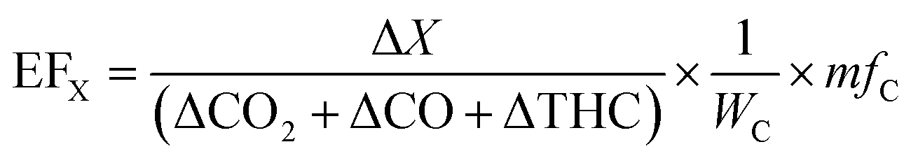 | (2) |
3. Results and discussion
3.1 TD/GC/MS calibration with standard mixtures
To interpret the full scan TICs collected from biomass burning emission samples, calibration experiments described in Section 2.2 were conducted. Fig. 1A shows the resulting calibration for C* as a function of GC elution time for a suite of standard compounds including straight chain alkanes, PAHs, methoxyphenols, levoglucosan and saturated acids. Within a compound series, more volatile compounds (higher C*) elute earlier. The plot suggests that compounds in the PAH standard can be described by a similar C* calibration curve as n-alkanes indicated by similar slopes, intercepts and R2 values (logC* = −0.41 × retention time + 13.6, R2 = 0.97, fits not pictured in Fig. 1A). However, separate curves may be necessary for methoxyphenols and saturated acids. These differences may be driven at least partly by differences in polarity53 that shift elution times for the alkanes/PAHs relative to the other classes of compounds explored here.
 | ||
| Fig. 1 (A) Estimated saturation concentration, C*, plotted against GC retention time for calibration compounds – n-alkanes, PAHs, methoxyphenols, saturated acids and levoglucosan (delineated by color). Vertical dashed lines denote the boundaries of C* bins where the number at the top of the bins indicate logC* for each bin. Error bars show ± one standard deviation of 4 replicates of alkane standards. (B) Response factor for calibration compounds – n-alkanes, methoxyphenols (MPs), PAHs and levoglucosan (sugar) (delineated by color) as a function of the n-alkane equivalent eluting carbon number bin. The solid black line represents a degree 3 polynomial fitted to describe the variation in response factors of n-alkanes (equation: y = 1.7–0.1x − 0.01x2 + 0.0004x3) while the dotted black lines show the 95% confidence interval on the fit. The grey boxes in panel A are where the calibrated (labels on top of bin ranges) and estimated C* overlap. Note: C* vs. GC retention time data for saturated acids were collected fortuitously from another calibration exercise; a separate calibration for response factor was not completed and hence this data is missing from (B). | ||
The vertical dashed lines in Fig. 1A show the boundaries of the C* bins defined based on n-alkane retention times. The bins are defined such that compounds half a decade greater and lesser than the bin center in saturation concentration are included in a given bin. For example, the bin representing logC* = 5 includes all compounds with 4.5 ≤ logC* < 5.5. Material eluting after 38 minutes in the chromatogram cannot be resolved further and is lumped with C* = 10−2 μg m−3 bin, which will be in the condensed phase under essentially all atmospheric conditions. Quantifying emissions in bins up to log10C* = 6 captures S/I-VOCs, which likely represent a substantial fraction of SOA precursors.12Fig. 1A illustrates how compounds from the TIC (including UCM) can be ascribed to C* bins based on the corresponding n-alkane eluting in that bin.
Fig. 1B shows response factors for different classes of compounds as a function of n-alkane carbon bins. As shown in Fig. 1A, the n-alkane carbon bin number of a compound is based on the GC retention time of the corresponding eluting n-alkane. In this way, methoxyphenols, PAHs and levoglucosan are presented on the same ‘equivalent’ n-alkane basis. The response factors were derived from calibration runs where known amounts of standard compounds are spiked onto a sample medium along with an internal standard and analyzed by the TD/GC/MS. We fit a cubic function to describe the variation in response factor of n-alkanes vs. n-alkane bin (used as a proxy for GC retention time); fit parameters are given in Fig. 1 caption). Data across four calibration runs are included in this fit (error bars show standard deviation of replicates). The response factors for the n-alkanes calculated from these calibration experiments were consistent as indicated by the coefficient of variation (0.12 ± 0.08) calculated on the average response factors across the calibration experiments (N = 4). Response factors show a marked variation across the carbon number range, with average response factors for C10 to C19 and C31 to C40n-alkanes 111% and 416% greater than those for C20 to C30n-alkanes. The compounds in the methoxyphenol standard eluted in the same retention time intervals as C10–C14 straight-chained alkanes and show a response factor larger than corresponding alkanes eluting in these bins by an average of 27% ± 18%. Levoglucosan also had a response factor 20% larger than the corresponding eluting n-alkane (C15). In contrast, the PAHs elute later, across a larger range (C15–C33 alkanes) and with a lower response factor compared to the alkanes by an average of 48% ± 8%. The confidence intervals on the n-alkane response factor fit generally included the response factors from the other calibration compounds explored here, suggesting that we can constrain the uncertainty introduced by varying response factors across compound classes.
3.2 Particulate matter emission factors
Fig. 2 demonstrates the diverse types of biomass burning (field, burnhut and RWC) studied by showing test-averaged PM2.5 EF (from integrated filter measurements) plotted against MCE. PM2.5 EFs are inversely related with MCE across the different sources, as has been typically observed.54,55 Amongst the sources studied here, field burns had the highest average MCE (0.94 ± 0.02) while burn hut burns were the least efficient (MCE ∼ 0.79), resulting in larger PM2.5 EFs. An MCE threshold of 0.9 has often been used to demarcate smoldering vs. flaming combustion conditions56 indicating burnhut combustion was primarily smoldering while the others were mostly flaming conditions. The RWC-high phase had the lowest average PM2.5 EF (4.4 ± 3.3 g kg of fuel−1). PM2.5 EFs for field burns were consistent with other work where a range of 6.26 g kg of fuel−1 (crop residue) to 15.3 g kg of fuel−1 (boreal forest) was reported.55 PM2.5 EFs from RWC emissions overlapped with observations from literature where PM2.5 EFs of 2.2 ± 1.2 g kg of fuel−1 was recorded across various fuels.57 Fig. S3† shows OC and EC EFs plotted against MCE where OC EFs are inversely related to MCE (like PM2.5 EFs) while EC EFs generally increase with MCE. PM and OC EFs from the combustion sources in this study span two orders of magnitude indicating diversity in emission characteristics. PM2.5 mass is dominated by OC with OC/PM ratios of 54 ± 16%, 63 ± 9% and 66 ± 7% for RWC, field and burn hut, respectively. EC/PM was significantly more variable and largest for RWC (10 ± 8%) and comparable for field and burnhut (4 ± 4% and 2 ± 2% respectively). OM/OC ratios were estimated as: (PM EF−EC EF)/OC EF in the absence of more detailed chemical information (e.g. parameterization of aerosol mass spectra58). The average OM/OC ratio across all experiments was 1.53 ± 0.18 consistent with literature values;59,60 this average was applied to OC EFs to infer OM EFs. The estimated OM EF + EC EF is plotted against PM2.5 EF in Fig. S4.† In this study we emphasize the consistency in relationship between PM2.5 and MCE across the different types of biomass burning and conditions rather than the absolute EF values. Fig. 2 shows that the samples included in this evaluation of the volatility distribution estimation method span a range of biomass burning emissions. However future work should systematically vary combustion and sampling parameters to explore sensitivities not explicitly considered here. | ||
| Fig. 2 PM2.5 emission factors (PM2.5 EF) as function of modified combustion efficiency (MCE) for different source emissions – burnhut, field, RWC phases (delineated by color). Faded markers represent test-averaged observations from individual integrated filter measurements while darker markers show the average PM2.5 EF and MCE from an emissions source type with the error bars denoting the standard deviation across individual tests. | ||
3.3 Volatility distribution profiles of biomass burning sources
Fig. 3A shows normalized volatility distributions (fi) inferred from TD/GC/MS chromatograms of filter-in-tube biomass burning samples. The volatility distributions are presented as the mass fraction in log-spaced C* bins applying the method described in Section 2.4. To compare the volatility distributions of different source emissions we group the bins into the three volatility ranges labeled on the plot: IVOC, SVOC and LVOC. IVOCs dominate the volatility distribution with average contributions of 75 ± 9%, 80 ± 6%, 84 ± 15% and 90 ± 15% of total organic emissions for burnhut, field, RWC – high and RWC – startup, respectively. The bins with logC* = 6 dominate across the different combustion sources, with 50−80% of total IVOC emissions contained in this bin. SVOCs represent 13 ± 3%, 6 ± 1%, 13 ± 2% and 8 ± 1% of total organic emissions for burnhut, field, RWC – high and RWC – startup, respectively. Finally, LVOCs contribute 12 ± 4%, 14 ± 9%, 3 ± 2% and 1 ± 1% for burn hut, field, RWC – high and RWC – startup, respectively. The differences in contributions to LVOCs and SVOCs across the different combustion sources could play important differences in POA partitioning behavior. For example, a higher OA concentration will be required for RWC – high emissions to achieve the same particle mass fraction relative to field emissions because of higher SVOC and lower LVOC contributions, assuming that all other atmospheric conditions are the same.
 | ||
| Fig. 3 (A) Volatility distributions of biomass burning combustion sources (burnhut, field, RWC – high and RWC – startup; delineated by color) presented as mass fraction in each log-spaced saturation concentration (logC*) bin. The mass fraction shown in each bin is the average bin mass from replicate (N = 3) samples while the error bars show the standard deviations of replicates. (B) Biomass burning source emission (delineated by color) volatility distributions presented as emission factors by normalizing the mass emitted in each logC* bin by amount of fuel burnt. The bin emission factor showed in each bin is the average bin emission factor from replicate (N = 3) samples while the error bars show the standard deviations of replicates. | ||
Fig. S5† shows paired scatter plots of the mass fractions in each logC* bin for the different source emissions to compare the distributions across burn types. Since the contribution in the logC* = 6 bin is larger by more than a factor of 3 than the other bins, linear fits would be influenced by high leveraging. Instead, we calculate the root mean square error (RMSE) to the 1:1 line to quantify deviations from complete agreement, indicated by an RMSE of 0, between two distributions and interpret the RMSEs in a relative manner. The RMSE was calculated in the vertical/horizontal direction, both giving the same result, as well as orthogonal to the 1:1 line however only the latter is printed in Fig. S5† since the relative differences were the same across methods. According to this metric, the most similar distribution pairs were RWC high – RWC startup, field – RWC high and burn hut – field. In contrast, the burnhut – RWC startup comparison had the least similar distribution by this metric.
In Fig. 3B we show the volatility distributions as EFs by normalizing the mass emitted in each logC* bin by the amount of fuel burnt as described in eqn (1). The bin mass emission factors span two orders of magnitude across the biomass burning combustion sources indicating variation consistent with PM emission factors discussed in Section 3.3. This indicates that fuel composition and combustion conditions influence contributions to logC* bins and PM from integrated filter measurements.
3.4 Comparison of volatility distributions with literature
Fig. S6† shows comparisons of the volatility distributions shown in Fig. 3 with the distributions derived in May et al.11 The measurement range in May et al.11 spans logC* = −2 to 4 bins and thus our distributions are re-normalized after removing the contributions from the logC* = 5 and 6 bins to allow direct comparisons. Fig. S7† shows scatter plots of mass fractions in each logC* bin from our source emissions and May et al., with the largest differences arising from the bins: −2, 3 and 4. However, RMSEs calculated to the 1:1 line were of similar magnitude across our various source distributions when compared to the May et al. distribution. Therefore, the variation within our different source type distributions is similar to that between ours and the May et al. distribution, and thus our distributions are similar to the May et al. distribution.
To explore the implications of differences in volatility distributions, Fig. 4A shows the particle mass fraction (Xp) predicted from the partitioning equation (eqn (1)) as a function of COA. We used the volatility distributions shown in Fig. S6† (normalized after removing logC* bins 5 and 6) to derive these curves to enable comparison with partitioning behavior from May et al.11 . Fig. S8† shows both the partitioning curves generated from these truncated volatility distributions and with those in Fig. 3A (including logC* bins 5 and 6) for comparison, with the latter showing lower Xp values, especially at lower COA. Across the different source types, we observe maximum differences in predicted Xp at lower COA, with decreasing divergence for increasing COA. This is due to the relatively larger differences in LVOC and SVOC contributions across the different source emissions. As the OA concentration increases, the differences in the contributions of lower and semi-volatile compounds matter less to POA partitioning as these bins are saturated. Between the RWC phases, the average predicted Xp for startup conditions is greater than that for high fire conditions by a maximum relative difference of 12.9% (at 5.8 μg m−3), which decreases to <10% at 68 μg m−3 with increases in COA leading to further decreases in difference of Xp. This indicates that there are only minor differences in the predicted partitioning between the RWC phases. The difference in average predicted Xp is larger between burnhut and field burn conditions with a 40% difference at 10 μg m−3, reducing to 24% at 100 μg m−3 and <10% at 790 μg m−3. The greater differences here are mainly driven by larger Xp predictions from one replicate sorbent sample (relative to the other two) taken under field conditions. The difference in predicted Xp between burnhut and the other field samples (thin blue lines in a lower clustering in Fig. 4A) are <5% across all modeled COA. Thus, the Xp predicted for most samples collected from burnhut and field burn emissions are generally consistent, even though PM2.5 EFs are >2 larger for burnhut compared to field emissions (Fig. 2). Finally, the difference in average predicted Xp between RWC – high and burnhut conditions is 43% at 10 μg m−3 and decreases to 13% at 100 μg m−3. Overall, we see that the difference in Xp is about 10% (or lower) across the biomass burning sources at COA larger than 100 μg m−3 indicating relative similarity in volatility distributions and that partitioning is less sensitive to variations in distributions at higher concentrations.
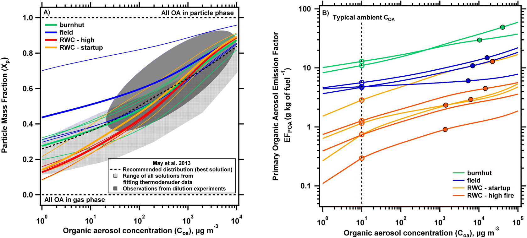 | ||
| Fig. 4 (A) Partitioning plot showing the particle mass fraction (Xp) calculated using eqn (1) and volatility distributions shown in Fig. S6† (omitting logC* bins 5 and 6 and re-normalized to match observations from May et al. (2013a)) vs. organic aerosol concentration (COA). The biomass burning sources are delineated by color, with the thin lines showing the predicted partitioning from individual experiments and the thicker lines showing the average for each biomass burning type. Also plotted are observations from May et al. (2013a): (1) range of observations from chamber dilution experiments (dark gray oval), (2) predictions from the range of feasible solutions obtained from fitting thermodenuder data (light gray region), (3) predictions using their recommended biomass burning distribution (at 25 °C) (dotted black line). (B) Primary organic aerosol emission factor (POA EF) as a function of organic aerosol concentration (COA) derived using the partitioning equation and the volatility distributions shown in Fig. 3B (including all bins). The predicted partitioning for each replicate tube sample is shown with an individual line with each biomass burning type delineated by color. The closed circles indicate the POA EFs measured at the sampling concentration of each experiment while the open circles use the volatility distributions to predict POA EF at COA = 10 μg m−3 to represent an equivalent EF at dilute/ambient conditions. | ||
Fig. 4A also plots gas–particle partitioning behavior from distributions developed by May et al. To compare predicted partitioning behavior from the current work, we consider three sets of results from this study: (1) observed partitioning from chamber dilution experiments; (2) predictions made from the range of feasible solutions obtained from fitting thermodenuder data; (3) predictions from the study's ‘best overall’ biomass burning distribution (at 25 °C). We see that our gas–particle partitioning profiles are generally well constrained within observations from dilution experiments (dark gray oval) and the range of statistically acceptable solutions from fitting thermodenuder data (light gray region) except for one field profile. The average burnhut profiles compared to the best solution profile from May et al. (dotted black line in Fig. 4A) shows a difference in predicted Xp of <5% throughout the modeled COA range, indicating close agreement in distributions from distinct methods but relatively consistent combustion methods (lab burns of diverse biomass types). Consistency in the predicted profiles from our study and May et al. support the viability of deriving volatility distributions by analyzing filter-in-tube sorbents using a TD/GC/MS for biomass burning emissions.
Fig. 4B shows partitioning plots in terms of POA emission factor as a function of COA using the volatility distributions presented in Fig. 3B along with the partitioning equation. Also shown are the POA EFs measured at OA sampling concentrations (which ranged between 1300 and 40000 μg m−3) represented by the closed markers. These concentrations are comparable to those in near-field fire plumes and much higher than typical ambient concentrations. The differences in combustion conditions and configurations (e.g. open vs. closed combustion) and fuel compositions result in POA emission factor profiles spanning two orders of magnitude for the different biomass burning sources (POA EFs range from 0.9–49 g kg of fuel−1). Based on the partitioning equation, smaller POA emission factors are expected at lower COA such as those found at ambient conditions. In Fig. 4B we show the estimated POA emission factor at 10 μg m−3 for individual test data using open markers. 10 μg m−3 is chosen as an arbitrary dilute/ambient concentration and was also used to model ambient scenarios in the analysis of Robinson et al. (2010). We acknowledge that ambient concentrations may be higher in fire impacted environments like those from woodstove emissions (tens of μg m−3) and wildfire (tens or hundreds of μg m−3) but choose this value for illustrative purposes. Predicted POA emission factors at 10 μg m−3 are 56−77%, 20–62% and 50–77% lower than POA emission factors measured at the sampling concentration for burnhut, field and RWC emissions respectively, demonstrating the dominant contribution of I/SVOCs on POA emissions. These ranges are a function of both volatility distributions and sampling conditions. If the volatility distributions are known, POA EFs can be estimated under any sampling conditions.
4. Implications, limitations, and future work
In this work, we quantified the contributions of S/I-VOCs from biomass burning sources with different combustion conditions and fuel types in the VBS framework. We measured both gas and particle phase concentrations of emitted organic aerosol by sampling on sorbent tubes inset with quartz filters, which allowed the observation of a larger range of volatility species (−2 ≤ logC* ≤ 6) than either sampling medium alone. This method was novel in its application for characterizing biomass burning emissions. We showed that, while there were notable differences in volatility distributions across burn types, the predicted partitioning using this method is consistent with previous observations from chamber dilution and thermodenuder experiments.11 This agreement highlights the potential of predicting partitioning behavior of biomass burning emissions using filter-in-tube sorbent samples. The main advantages of using this method are: (1) the derived volatility distributions are more comprehensive since both gas and particle phase organics are measured together; (2) estimations can be made based on the analysis of a single sample using standard TD/GC/MS analytical instrumentation, and; (3) POA mass distributions can be constrained in the lowest volatility bins without the requirement of equilibrium with the gas phase during sampling. Gas–particle equilibrium is a requirement in dilution-based studies (which do not incorporate kinetic modeling) aimed at estimating volatility distributions and is challenging, especially at lower concentrations.12 Further, this relatively simple sampling approach makes in situ measurements possible allowing future studies to characterize in-field measurements of the actual sources as opposed to relying on laboratory simulations.
An advantage of this approach is the potential to quantify emissions in higher C* bins (logC* = 5, 6), which may allow for more accurate parameterizations of SOA formation potentials or gas–particle partitioning at very high sampling concentrations (100−1000 μg m−3). The volatility distributions derivable from this method can also be useful for application in CTMs, the performance of which have previously benefitted from the addition of volatility information.61–63 CTMs are important tools that can inform policy and regulations and thus, the addition of these distributions to model OA in CTMs can result in improved predictions relative to traditional approaches.
The volatility distributions derived for the biomass burning sources sampled here were generally consistent. IVOCs dominated the volatility distributions, accounting for 75–90% of the total contribution across the biomass burning sources, while SVOCs and LVOCs were responsible for 6–13% and 1–12%, respectively. Consistency in volatility distributions and predicted partitioning across the sources was observed despite PM emission factors spanning two orders of magnitude. However, substantial differences were also observed in the SVOC and LVOC contributions across the sources studied, which have implications on POA partitioning behavior. The influence on POA partitioning behavior is most pronounced at lower organic loadings. Although we did not perform molecular chemical speciation, the variability in composition from different types of biomass smoke has been observed previously.64–66 Recent work has also shown the key influence of combustion temperature/phase on VOC emission characteristics.67 The partitioning behavior of biomass burning emissions is governed by thousands of semi-volatile species with varying chemical identities, vapor pressures and mixing properties. However, when considered together, the overall partitioning behavior of all these mixtures was similar enough to be represented using similar volatility distributions. In our analyses, we binned the TICs based on standard compound behavior. However, there is a potential to deconvolve the mass spectra further and extract more detailed chemical information. This chemical information can be used to inform yields for SOA production, with applications in air quality models or source apportionment. One of the key assumptions of this method is that compounds in the UCM behave like n-alkanes and have similar response factors. Analysis of calibration samples showed that polynomial fits describing response factors for a set of standard calibration compound classes were roughly constrained within the variation between different compounds. The resulting fit was best constrained between C15 and C30 while predicted response factors for later- and earlier-eluting compounds were more uncertain. However, combustion of biomass can also emit oxygenated IVOCs68 which may not be measured by the TD/GC/MS or remain in an unresolved state. The application of hydrocarbon response factors to these compounds may underestimate the mass in the IVOC bins as polar compounds tended to have lower response factors than hydrocarbons. Another key assumption involves correction of the organic mass estimated using thermal desorption gas chromatography mass spectrometry (TD/GC/MS) chromatograms with organic carbon (OC) filter measurements. The need for this correction factor likely arises because oxygenated compounds may not elute and thus are omitted from the UCM in chromatograms but are collected on filter samples. Our correction assumes an even bias across the volatility range; this assumption cannot be tested with our methods but may be probed using more advanced gas chromatography methods. More complete speciation of organic compounds present in the gas and particle phase of combustion emissions is increasingly possible with the development of novel instrumentation and techniques.39,68,69 Future work should derive POA volatility using these resources to validate these key assumptions in this method.
Conflicts of interest
There are no conflicts of interest to declare.Acknowledgements
The views expressed in this article are those of the authors and do not necessarily represent the views or policies of the U.S. Environmental Protection Agency. AS and AG acknowledge support from the National Science Foundation under Grant No. CBET-13-51721 and an NSF INTERN supplement that supported an internship for AS at the US EPA. The authors acknowledge Johanna Aurell and Brian Gullet for assistance with field sample collection, Larry Virtaranta, Alina Brashear and Aranya Ahmed for assistance with laboratory sample collection, and Bakul Patel and Emily Li for assistance with sample analysis.References
- I. P. C. C., The Physical Science Basis. Contribution of Working Group I to the Fifth Assessment Report of the Intergovernmental Panel on Climate Change, Cambridge University Press, Cambridge, United Kingdom and New York, NY, USA, Geneva, Switzerland, 2014, p. 1535 Search PubMed.
- S. Fuzzi, U. Baltensperger, K. Carslaw, S. Decesari, H. Denier van der Gon, M. C. Facchini, D. Fowler, I. Koren, B. Langford, U. Lohmann, E. Nemitz, S. Pandis, I. Riipinen, Y. Rudich, M. Schaap, J. G. Slowik, D. V. Spracklen, E. Vignati, M. Wild, M. Williams and S. Gilardoni, Particulate matter, air quality and climate: lessons learned and future needs, Atmospheric Chem. Phys., 2015, 15, 8217–8299 CrossRef CAS.
- C. A. I. Pope, M. Ezzati and D. W. Dockery, Fine-Particulate Air Pollution and Life Expectancy in the United States, N. Engl. J. Med., 2009, 360, 376–386 CrossRef CAS PubMed.
- Health Effects Institute and State of Global Air, A Special Report on Global Exposure to Air Pollution and its Disease Burden, Boston, MA, 2019 Search PubMed.
- S. Chowdhury, S. Dey, S. Guttikunda, A. Pillarisetti, K. R. Smith and L. D. Girolamo, Indian annual ambient air quality standard is achievable by completely mitigating emissions from household sources, Proc. Natl. Acad. Sci., 2019, 116, 10711–10716 CrossRef CAS PubMed.
- L. Conibear, E. W. Butt, C. Knote, S. R. Arnold and D. V. Spracklen, Residential energy use emissions dominate health impacts from exposure to ambient particulate matter in India, Nat. Commun., 2018, 9, 617 CrossRef PubMed.
- T. C. Bond, D. G. Streets, K. F. Yarber, S. M. Nelson, J. H. Woo and Z. Klimont, A technology-based global inventory of black and organic carbon emissions from combustion, J. Geophys. Res. Atmospheres, 2004, 109, 1–43 CrossRef.
- T. C. Bond, S. J. Doherty, D. W. Fahey, P. M. Forster, T. Berntsen, B. J. DeAngelo, M. G. Flanner, S. Ghan, B. Kärcher, D. Koch, S. Kinne, Y. Kondo, P. K. Quinn, M. C. Sarofim, M. G. Schultz, M. Schulz, C. Venkataraman, H. Zhang, S. Zhang, N. Bellouin, S. K. Guttikunda, P. K. Hopke, M. Z. Jacobson, J. W. Kaiser, Z. Klimont, U. Lohmann, J. P. Schwarz, D. Shindell, T. Storelvmo, S. G. Warren and C. S. Zender, Bounding the role of black carbon in the climate system: A scientific assessment, J. Geophys. Res. Atmospheres, 2013, 118, 5380–5552 CrossRef CAS.
- C. Wiedinmyer, S. K. Akagi, R. J. Yokelson, L. K. Emmons, J. A. Al-Saadi, J. J. Orlando and A. J. Soja, The Fire INventory from NCAR (FINN): a high resolution global model to estimate the emissions from open burning, Geosci. Model Dev., 2011, 4, 625–641 CrossRef.
- M. O. Andreae and D. Rosenfeld, Aerosol–cloud–precipitation interactions. Part 1. The nature and sources of cloud-active aerosols, Earth-Sci. Rev., 2008, 89, 13–41 CrossRef.
- A. A. May, E. J. T. Levin, C. J. Hennigan, I. Riipinen, T. Lee, J. L. Collett, J. L. Jimenez, S. M. Kreidenweis and A. L. Robinson, Gas-particle partitioning of primary organic aerosol emissions: 3. Biomass burning, J. Geophys. Res. Atmospheres, 2013, 118, 11327–11338 CrossRef CAS.
- A. P. Grieshop, J. M. Logue, N. M. Donahue and A. L. Robinson, Laboratory investigation of photochemical oxidation of organic aerosol from wood fires 1: measurement and simulation of organic aerosol evolution, Atmospheric Chem. Phys., 2009, 9, 1263–1277 CrossRef CAS.
- A. L. Robinson, N. M. Donahue, M. K. Shrivastava, E. A. Weitkamp, A. M. Sage, A. P. Grieshop, T. E. Lane, J. R. Pierce and S. N. Pandis, Rethinking Organic Aerosols: Semivolatile Emissions and Photochemical Aging, Science, 2007, 315, 1259–1262 CrossRef CAS PubMed.
- M. K. Shrivastava, E. M. Lipsky, C. O. Stanier and A. L. Robinson, Modeling semivolatile organic aerosol mass emissions from combustion systems, Environ. Sci. Technol., 2006, 40, 2671–2677 CrossRef CAS PubMed.
- A. L. Robinson, A. P. Grieshop, N. M. Donahue and S. W. Hunt, Updating the Conceptual Model for Fine Particle Mass Emissions from Combustion Systems, J. Air Waste Manag. Assoc., 2010, 60, 1204–1222 CrossRef CAS PubMed.
- H. A. C. Denier van der Gon, R. Bergström, C. Fountoukis, C. Johansson, S. N. Pandis, D. Simpson and A. J. H. Visschedijk, Particulate emissions from residential wood combustion in Europe – revised estimates and an evaluation, Atmospheric Chem. Phys., 2015, 15, 6503–6519 CrossRef CAS.
- J. F. Pankow, An absorption model of gas/particle partitioning of organic compounds in the atmosphere, Atmos Env, 1994, 28, 185 CrossRef CAS.
- N. M. Donahue, A. L. Robinson, C. O. Stanier and S. N. Pandis, Coupled partitioning, dilution, and chemical aging of semivolatile organics, Env. Sci Technol, 2006, 40, 2635–2643 CrossRef CAS PubMed.
- B. N. Murphy, N. M. Donahue, A. L. Robinson and S. N. Pandis, A naming convention for atmospheric organic aerosol, Atmos. Chem. Phys., 2014, 14(11), 5825–5839 CrossRef.
- N. M. Donahue, J. H. Kroll, S. N. Pandis and A. L. Robinson, A two-dimensional volatility basis set – Part 2: Diagnostics of organic-aerosol evolution, Atmospheric Chem. Phys., 2012, 12, 615–634 CrossRef CAS.
- Y. Morino, S. Chatani, K. Tanabe, Y. Fujitani, T. Morikawa, K. Takahashi, K. Sato and S. Sugata, Contributions of Condensable Particulate Matter to Atmospheric Organic Aerosol over Japan, Environ. Sci. Technol., 2018, 52, 8456–8466 CrossRef CAS PubMed.
- Y. Zhao, C. J. Hennigan, A. A. May, D. S. Tkacik, J. A. de Gouw, J. B. Gilman, W. C. Kuster, A. Borbon and A. L. Robinson, Intermediate-volatility organic compounds: a large source of secondary organic aerosol, Env. Sci Technol, 2014, 48, 13743–13750 CrossRef CAS PubMed.
- J. J. Schauer, M. J. Kleeman, G. R. Cass and B. R. T. Simoneit, Measurement of Emissions from Air Pollution Sources. 2. C 1 through C 30 Organic Compounds from Medium Duty Diesel Trucks, Environ. Sci. Technol., 1999, 33, 1578–1587 CrossRef CAS.
- J. J. Schauer, M. J. Kleeman, G. R. Cass and B. R. T. Simoneit, Measurement of Emissions from Air Pollution Sources. 3. C 1 −C 29 Organic Compounds from Fireplace Combustion of Wood, Environ. Sci. Technol., 2001, 35, 1716–1728 CrossRef CAS PubMed.
- C. J. Gaston, F. D. Lopez-Hilfiker, L. E. Whybrew, O. Hadley, F. McNair, H. Gao, D. A. Jaffe and J. A. Thornton, Online molecular characterization of fine particulate matter in Port Angeles, WA: Evidence for a major impact from residential wood smoke, Atmos. Environ., 2016, 138, 99–107 CrossRef CAS.
- M. D. Hays, C. D. Geron, K. J. Linna, N. D. Smith and J. J. Schauer, Speciation of Gas-Phase and Fine Particle Emissions from Burning of Foliar Fuels, Environ. Sci. Technol., 2002, 36, 2281–2295 CrossRef CAS PubMed.
- L. R. Mazzoleni, B. Zielinska and H. Moosmüller, Emissions of Levoglucosan, Methoxy Phenols, and Organic Acids from Prescribed Burns, Laboratory Combustion of Wildland Fuels, and Residential Wood Combustion, Environ. Sci. Technol., 2007, 41, 2115–2122 CrossRef CAS PubMed.
- A. A. May, A. A. Presto, C. J. Hennigan, N. T. Nguyen, T. D. Gordon and A. L. Robinson, Gas-particle partitioning of primary organic aerosol emissions: (1) Gasoline vehicle exhaust, Atmos. Environ., 2013, 77, 128–139 CrossRef CAS.
- X. Li, T. R. Dallmann, A. A. May, D. S. Tkacik, A. T. Lambe, J. T. Jayne, P. L. Croteau and A. A. Presto, Gas-Particle Partitioning of Vehicle Emitted Primary Organic Aerosol Measured in a Traffic Tunnel, Env. Sci Technol, 2016, 50(22), 12146–12155 CrossRef CAS PubMed.
- S. H. Jathar, N. Sharma, A. Galang, C. Vanderheyden, M. Takhar, A. W. H. Chan, J. R. Pierce and J. Volckens, Measuring and modeling the primary organic aerosol volatility from a modern non-road diesel engine, Atmos. Environ., 2019, 117221 Search PubMed.
- A. P. Grieshop, M. A. Miracolo, N. M. Donahue and A. L. Robinson, Constraining the Volatility Distribution and Gas-Particle Partitioning of Combustion Aerosols Using Isothermal Dilution and Thermodenuder Measurements, Environ. Sci. Technol., 2009, 43, 4750–4756 CrossRef CAS PubMed.
- I. Riipinen, J. R. Pierce, N. M. Donahue and S. N. Pandis, Equilibration time scales of organic aerosol inside thermodenuders: Evaporation kinetics versus thermodynamics, Atmos. Environ., 2010, 44, 597–607 CrossRef CAS.
- R. Saleh, A. Shihadeh and A. Khlystov, On transport phenomena and equilibration time scales in thermodenuders, Atmospheric Meas. Tech., 2011, 4, 571–581 CrossRef CAS.
- P. K. Saha, A. Khlystov and A. P. Grieshop, Determining Aerosol Volatility Parameters Using a “Dual Thermodenuder” System: Application to Laboratory-Generated Organic Aerosols, Aerosol Sci. Technol., 2015, 49, 620–632 CrossRef CAS.
- Y. Fujitani, K. Sato, K. Tanabe, K. Takahashi, J. Hoshi, X. Wang, J. C. Chow and J. G. Watson, Volatility Distribution of Organic Compounds in Sewage Incineration Emissions, Env. Sci Technol, 2020, 11 Search PubMed.
- A. A. Presto, C. J. Hennigan, N. T. Nguyen and A. L. Robinson, Determination of Volatility Distributions of Primary Organic Aerosol Emissions from Internal Combustion Engines Using Thermal Desorption Gas Chromatography Mass Spectrometry, Aerosol Sci. Technol., 2012, 46, 1129–1139 CrossRef CAS.
- Y. Zhao, N. T. Nguyen, A. A. Presto, C. J. Hennigan, A. A. May and A. L. Robinson, Intermediate Volatility Organic Compound Emissions from On-Road Gasoline Vehicles and Small Off-Road Gasoline Engines, Env. Sci. Technol., 2016, 50, 4554–4563 CrossRef CAS PubMed.
- Y. Zhao, N. T. Nguyen, A. A. Presto, C. J. Hennigan, A. A. May and A. L. Robinson, Intermediate Volatility Organic Compound Emissions from On-Road Diesel Vehicles: Chemical Composition, Emission Factors, and Estimated Secondary Organic Aerosol Production, Env. Sci. Technol., 2015, 49, 11516–11526 CrossRef CAS PubMed.
- D. R. Worton, G. Isaacman, D. R. Gentner, T. R. Dallmann, A. W. H. Chan, C. Ruehl, T. W. Kirchstetter, K. R. Wilson, R. A. Harley and A. H. Goldstein, Lubricating Oil Dominates Primary Organic Aerosol Emissions from Motor Vehicles, Environ. Sci. Technol., 2014, 48, 3698–3706 CrossRef CAS PubMed.
- J. Jiang, I. El-Haddad, S. Aksoyoglu, G. Stefenelli, A. Bertrand, N. Marchand, F. Canonaco, J.-E. Petit, O. Favez, S. Gilardoni, U. Baltensperger and A. S. H. Prévôt, Influence of Biomass Burning Vapor Wall Loss Correction on Modelingorganic Aerosols in Europe by CAMx v6.50, Atmospheric Sciences, 2020 Search PubMed.
- G. Ciarelli, I. El Haddad, E. Bruns, S. Aksoyoglu, O. Möhler, U. Baltensperger and A. S. H. Prévôt, Constraining a hybrid volatility basis-set model for aging of wood-burning emissions using smog chamber experiments: a box-model study based on the VBS scheme of the CAMx model (v5.40), Geosci. Model Dev., 2017, 10, 2303–2320 CrossRef CAS.
- G. Ciarelli, S. Aksoyoglu, I. El Haddad, E. A. Bruns, M. Crippa, L. Poulain, M. Äijälä, S. Carbone, E. Freney, C. O'Dowd, U. Baltensperger and A. S. H. Prévôt, Modelling winter organic aerosol at the European scale with CAMx: evaluation and source apportionment with a VBS parameterization based on novel wood burning smog chamber experiments, Atmospheric Chem. Phys., 2017, 17, 7653–7669 CrossRef CAS.
- C. D. Cappa and J. L. Jimenez, Quantitative estimates of the volatility of ambient organic aerosol, Atmospheric Chem. Phys., 2010, 10, 5409–5424 CrossRef CAS.
- L. E. Hatch, A. Rivas-Ubach, C. N. Jen, M. Lipton, A. H. Goldstein and K. C. Barsanti, Measurements of I/SVOCs in biomass-burning smoke using solid-phase extraction disks and two-dimensional gas chromatography, Atmospheric Chem. Phys., 2018, 18, 17801–17817 CrossRef CAS.
- J. Aurell, B. K. Gullett, C. Pressley, D. G. Tabor and R. D. Gribble, Aerostat-lofted instrument and sampling method for determination of emissions from open area sources, Chemosphere, 2011, 85, 806–811 CrossRef CAS PubMed.
- X. Zhou, J. Aurell, W. Mitchell, D. Tabor and B. Gullett, A small, lightweight multipollutant sensor system for ground-mobile and aerial emission sampling from open area sources, Atmos. Environ., 2017, 154, 31–41 CrossRef CAS PubMed.
- B. Khan, M. D. Hays, C. Geron and J. Jetter, Differences in the OC/EC Ratios that Characterize Ambient and Source Aerosols due to Thermal-Optical Analysis, Aerosol Sci. Technol., 2012, 46, 127–137 CrossRef CAS.
- E. Grandesso, B. Gullett, A. Touati and D. Tabor, Effect of Moisture, Charge Size, and Chlorine Concentration on PCDD/F Emissions from Simulated Open Burning of Forest Biomass, Environ. Sci. Technol., 2011, 45, 3887–3894 CrossRef CAS PubMed.
- A. Holder, Black Carbon Emissions From Residential Wood Combustion Appliances, 2019, 76 Search PubMed.
- J. H. Kroll and J. H. Seinfeld, Chemistry of secondary organic aerosol: Formation and evolution of low-volatility organics in the atmosphere, Atmos. Environ., 2008, 42, 3593–3624 CrossRef CAS.
- J. F. Pankow and W. E. Asher, SIMPOL.1: a simple group contribution method for predicting vapor pressures and enthalpies of vaporization of multifunctional organic compounds, Atmospheric Chem. Phys., 2008, 8, 2773–2796 CrossRef CAS.
- R. Wathore, K. Mortimer and A. P. Grieshop, In-Use Emissions and Estimated Impacts of Traditional, Natural- and Forced-Draft Cookstoves in Rural Malawi, Environ. Sci. Technol., 2017, 51, 1929–1938 CrossRef CAS PubMed.
- G. Isaacman, D. R. Worton, N. M. Kreisberg, C. J. Hennigan, A. P. Teng, S. V. Hering, A. L. Robinson, N. M. Donahue and A. H. Goldstein, Understanding evolution of product composition and volatility distribution through in-situ GC × GC analysis: a case study of longifolene ozonolysis, Atmospheric Chem. Phys., 2011, 11, 5335–5346 CrossRef CAS.
- J. Jetter, Y. Zhao, K. R. Smith, B. Khan, T. Yelverton, P. DeCarlo and M. D. Hays, Pollutant Emissions and Energy Efficiency under Controlled Conditions for Household Biomass Cookstoves and Implications for Metrics Useful in Setting International Test Standards, Environ. Sci. Technol., 2012, 46, 10827–10834 CrossRef CAS PubMed.
- S. K. Akagi, R. J. Yokelson, C. Wiedinmyer, M. J. Alvarado, J. S. Reid, T. Karl, J. D. Crounse and P. O. Wennberg, Emission factors for open and domestic biomass burning for use in atmospheric models, Atmospheric Chem. Phys., 2011, 11, 4039–4072 CrossRef CAS.
- S. Collier, S. Zhou, T. B. Onasch, D. A. Jaffe, L. Kleinman, A. J. Sedlacek, N. L. Briggs, J. Hee, E. Fortner, J. E. Shilling, D. Worsnop, R. J. Yokelson, C. Parworth, X. Ge, J. Xu, Z. Butterfield, D. Chand, M. K. Dubey, M. S. Pekour, S. Springston and Q. Zhang, Regional Influence of Aerosol Emissions from Wildfires Driven by Combustion Efficiency: Insights from the BBOP Campaign, Environ. Sci. Technol., 2016, 50, 8613–8622 CrossRef CAS PubMed.
- S. Guofeng, W. Siye, W. Wen, Z. Yanyan, M. Yujia, W. Bin, W. Rong, L. Wei, S. Huizhong, H. Ye, Y. Yifeng, W. Wei, W. Xilong, W. Xuejun and T. Shu, Emission Factors, Size Distributions, and Emission Inventories of Carbonaceous Particulate Matter from Residential Wood Combustion in Rural China, Environ. Sci. Technol., 2012, 46, 4207–4214 CrossRef PubMed.
- M. R. Canagaratna, J. L. Jimenez, J. H. Kroll, Q. Chen, S. H. Kessler, P. Massoli, L. Hildebrandt Ruiz, E. Fortner, L. R. Williams, K. R. Wilson, J. D. Surratt, N. M. Donahue, J. T. Jayne and D. R. Worsnop, Elemental ratio measurements of organic compounds using aerosol mass spectrometry: characterization, improved calibration, and implications, Atmospheric Chem. Phys., 2015, 15, 253–272 CrossRef.
- E. J. T. Levin, G. R. McMeeking, C. M. Carrico, L. E. Mack, S. M. Kreidenweis, C. E. Wold, H. Moosmüller, W. P. Arnott, W. M. Hao, J. L. Collett and W. C. Malm, Biomass burning smoke aerosol properties measured during Fire Laboratory at Missoula Experiments (FLAME), J. Geophys. Res., 2010, 115, D18210 CrossRef.
- J. S. Reid, R. Koppmann, T. F. Eck and D. P. Eleuterio, A review of biomass burning emissions part II: intensive physical properties of biomass burning particles, Atmos. Chem. Phys., 2005, 5(3), 799–825 CrossRef CAS.
- T. E. Lane, N. M. Donahue and S. N. Pandis, Simulating secondary organic aerosol formation using the volatility basis-set approach in a chemical transport model, Atmos. Environ., 2008, 42, 7439–7451 CrossRef CAS.
- Q. J. Zhang, M. Beekmann, F. Drewnick, F. Freutel, J. Schneider, M. Crippa, A. S. H. Prevot, U. Baltensperger, L. Poulain, A. Wiedensohler, J. Sciare, V. Gros, A. Borbon, A. Colomb, V. Michoud, J.-F. Doussin, H. A. C. Denier van der Gon, M. Haeffelin, J.-C. Dupont, G. Siour, H. Petetin, B. Bessagnet, S. N. Pandis, A. Hodzic, O. Sanchez, C. Honoré and O. Perrussel, Formation of organic aerosol in the Paris region during the MEGAPOLI summer campaign: evaluation of the volatility-basis-set approach within the CHIMERE model, Atmospheric Chem. Phys., 2013, 13, 5767–5790 CrossRef.
- S. C. Farina, P. J. Adams and S. N. Pandis, Modeling global secondary organic aerosol formation and processing with the volatility basis set: Implications for anthropogenic secondary organic aerosol, J. Geophys. Res., 2010, 115, D09202 CrossRef.
- G. R. McMeeking, S. M. Kreidenweis, S. Baker, C. M. Carrico, J. C. Chow, J. L. Collett, W. M. Hao, A. S. Holden, T. W. Kirchstetter, W. C. Malm, H. Moosmüller, A. P. Sullivan and W. Cyle, Emissions of trace gases and aerosols during the open combustion of biomass in the laboratory, J. Geophys. Res. Atmospheres, 2009, 114, 1–20 CrossRef.
- P. M. Fine, G. R. Cass and B. R. T. Simoneit, Chemical Characterization of Fine Particle Emissions from Fireplace Combustion of Woods Grown in the Northeastern United States, Environ. Sci. Technol., 2001, 35, 2665–2675 CrossRef CAS PubMed.
- P. M. Fine, G. R. Cass and B. R. Simoneit, Chemical characterization of fine particle emissions from the wood stove combustion of prevalent United States tree species, Environ. Eng. Sci., 2004, 21, 705–721 CrossRef CAS.
- K. Sekimoto, A. R. Koss, J. B. Gilman, V. Selimovic, M. M. Coggon, K. J. Zarzana, B. Yuan, B. M. Lerner, S. S. Brown, C. Warneke, R. J. Yokelson, J. M. Roberts and J. de Gouw, High- and low-temperature pyrolysis profiles describe volatile organic compound emissions from western US wildfire fuels, Atmospheric Chem. Phys., 2018, 18, 9263–9281 CrossRef CAS.
- D. R. Gentner, G. Isaacman, D. R. Worton, A. W. H. Chan, T. R. Dallmann, L. Davis, S. Liu, D. A. Day, L. M. Russell, K. R. Wilson, R. Weber, A. Guha, R. A. Harley and A. H. Goldstein, Elucidating secondary organic aerosol from diesel and gasoline vehicles through detailed characterization of organic carbon emissions, Proc. Natl. Acad. Sci., 2012, 109, 18318–18323 CrossRef CAS PubMed.
- A. R. Koss, K. Sekimoto, J. B. Gilman, V. Selimovic, M. M. Coggon, K. J. Zarzana, B. Yuan, B. M. Lerner, S. S. Brown, J. L. Jimenez, J. Krechmer, J. M. Roberts, C. Warneke, R. J. Yokelson and J. de Gouw, Non-methane organic gas emissions from biomass burning: identification, quantification, and emission factors from PTR-ToF during the FIREX 2016 laboratory experiment, Atmos. Chem. Phys., 2018, 18, 3299–3319 CrossRef CAS.
Footnote |
| † Electronic supplementary information (ESI) available. See DOI: https://doi.org/10.1039/d2ea00080f |
| This journal is © The Royal Society of Chemistry 2023 |