Machine learning reaction barriers in low data regimes: a horizontal and diagonal transfer learning approach

Abstract

Machine learning (ML) models can, once trained, make reaction barrier predictions in seconds, which is orders of magnitude faster than quantum mechanical (QM) methods such as density functional theory (DFT). However, these ML models need to be trained on large datasets of typically thousands of expensive, high accuracy barriers and do not generalise well beyond the specific reaction for which they are trained. In this work, we demonstrate that transfer learning (TL) can be used to adapt pre-trained Diels–Alder barrier prediction neural networks (NNs) to make predictions for other pericyclic reactions using horizontal TL (hTL) and additionally, at higher levels of theory with diagonal TL (dTL). TL-derived predictions are possible with mean absolute errors (MAEs) below the accepted chemical accuracy threshold of 1 kcal mol⁻¹, a significant improvement on pre-TL prediction MAEs of >5 kcal mol⁻¹, and in extremely low data regimes, with as few as 33 and 39 new datapoints needed for hTL and dTL, respectively. Thus, hTL and dTL are powerful options for providing insight into reaction feasibility without the need for extensive high-throughput experimental or computational screening or large dataset generation for training bespoke ML models.

---

Introduction

Despite the extensive use of density functional theory (DFT) to calculate free energy activation barriers in reaction modelling,^1–3 machine learning (ML) methods have recently been developed that can predict these barriers.^4–14 Once trained, ML models can make barrier predictions in a fraction of the time it takes to compute them with DFT¹² and frequently obtain accuracies below the 1 kcal mol⁻¹ chemical accuracy threshold.^15,16 However, current ML barrier models need to be trained on vast datasets (typically thousands of datapoints) to make accurate predictions, requiring expensive QM calculations or large kinetic studies. Furthermore, model usability is currently limited to a specific region of chemical space; most models are local and struggle to extrapolate outside of the immediate chemical space of the data they are trained on.¹¹ Therefore, each time a model is required for a new reaction class typically thousands of new datapoints are needed, which is likely a much larger burden than calculating the barriers of interest directly with DFT. In addition, these models inherit the drawbacks associated with running DFT calculations and the approximations therein made.¹⁷ Hence, approaches are required to address these broad issues in applying ML to reaction barrier prediction.

One such approach is transfer learning (TL), whereby neural networks (NNs) are adapted to make accurate predictions for new tasks for which limited data is available.^18–20 TL takes a NN, including its calculated weights and biases, which has been pre-trained on a large quantity of source domain data and retrains a chosen number of hidden layers within the NNs architecture whilst freezing other layers. For any unfrozen layers, new weights and biases are optimised from their initial pre-trained values. This retraining of specific layers begins at a good estimation for these weights and biases provided by the pre-trained NN and thus, significantly reduces the computational cost of retraining. Additionally, this approach provides the ability to adapt the NNs for a new prediction task with very little data;²¹ the base NN is already trained on a large dataset and thus can be tuned via TL to make accurate predictions in much smaller data regimes (e.g., tens of datapoints) for new but related tasks.²² In contrast, building and training a new NN directly on such a low number of datapoints would risk overfitting to the training data²³ and provide poor generalisability to unseen data.^24,25

Recently, TL has become an area of increased interest within both organic and computational chemistry, with research utilising small, pre-existing datasets for solvation free energy, atomisation energy, and drug-like molecular torsion predictions.^26–32 However, until now, this technique has not been well defined. In this work we define three different classifications of TL in the context of free energy activation barrier prediction (Fig. 1), but these classes could equally be applied to other areas of chemical prediction. Notably, the prediction of activation barriers using TL has been explored for a diverse range of reactions across multiple levels of theory (LoT).^9,22,33 This, as defined herein, would be an example of Vertical TL (vTL); models trained to predict reaction barriers at one LoT, e.g., DFT, are adapted to make predictions at a higher LoT, e.g., CCSD(T), using only small amounts (<100 datapoints) of the higher quality data.^22,33 vTL provides a solution to the limited LoT accuracy of models built using DFT but does not improve generalisability. Instead, Horizontal TL (hTL), which takes a NN built for prediction on one specific chemical reaction and adapts this model to a new but related region of chemical space with small amounts of data, could be employed. This would improve predictions for the new reaction compared to the base model's predictions and provide prediction accuracy that would otherwise be unobtainable in these low data regimes. The final term defined in this work is Diagonal TL (dTL), which combines the benefits of both vTL and hTL to give an increased LoT accuracy for reaction barrier predictions whilst also increasing the base model's generalisability. All three TL approaches significantly reduce computational cost as they can be performed with limited new data. This makes them a viable option for early-stage predictions of activation barriers in reaction discovery, where they provide insights into reaction feasibility without the need for extensive high-throughput experimental or computational screening. As these activation barrier TL classifications have yet to be defined, it is a challenge to identify them within the literature, however use of both hTL and dTL in activation barrier prediction is, to the best of our knowledge, novel.

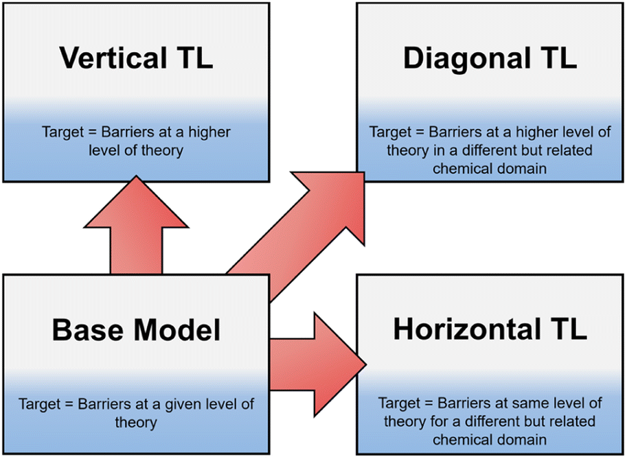Fig. 1 TL in reaction barrier prediction. vTL improves on LoT accuracy whilst not changing generalisability; hTL improves generalisability compared to the base model at the same LoT accuracy; dTL improves both generalisability and LoT accuracy.

In this work, we build ML models to predict the free energy activation barriers for a diverse selection of Diels–Alder reactions. We then demonstrate that hTL and dTL can be used to adapt the resulting NNs to make predictions for new reaction classes and improve their LoT accuracy using significantly less data (tens of datapoints) than was required in training the original NNs (750+ datapoints). The Diels–Alder reaction was selected due to its importance in pharmaceutical synthesis³⁴ in addition to the level of interest it has received over the years from the reaction modelling community.^35–40

The Diels–Alder reaction has previously been studied utilising ML approaches^41,42 but not in low data regimes (tens of datapoints).

Methodology

A diverse selection of Diels–Alder reactions (Fig. S1†) were enumerated using prevalent motifs throughout the literature, including a variety of intra/intermolecular and homo/hetero-Diels–Alder reactions,^43–53 as well as additional pericyclic reactions (e.g., tetrazine-based reactions).^54,55 Enumerations were performed using Schrödinger's Custom R-Group Enumeration⁵⁶ and all subsequent reactant and transition state (TS) structures conformationally searched using Schrödinger's MacroModel (version 12.7)^57,58 with the OPLS3e forcefield.⁵⁹ The lowest energy conformers for each structure were then optimised with two semi-empirical quantum mechanical (SQM) methods (AM1 ⁶⁰ and PM3 ⁶¹) and ωB97X-D/def2-TZVP^62,63 using Gaussian16 (Revision A.03 and C.01)^64,65 to generate AM1-DFT endo and exo datasets of 1065 and 1109 concerted reactions, respectively. Tetrazine-based Diels–Alder reactions were also optimised with DSD-PBEP86-D3(BJ)/def2-TZVP⁶⁶ to generate our dTL target dataset. Quasi-harmonic free energies were calculated with temperature (298.15 K) and concentration corrections (1 mol l⁻¹) using GoodVibes;⁶⁷ these energies were then used to calculate activation barriers for AM1, PM3, and DFT (Table S1†). Full activation barrier ranges and computational details are available in the ESI, Section 1.†

Several atomic and molecular physical organic chemical features were extracted for each SQM reactant and TS structure. The features are solely obtained from SQM structures; full descriptions of the features extracted for these SQM structures can be found in the ESI, Section 2, Tables S2 and S3.† These features were processed and standardised prior to training of the ML models. Each dataset was then randomly split into training and test sets. In this work, three scikit-learn⁶⁸ regression algorithms were used (ridge regression (Ridge), kernel ridge regression (KRR) with a radial basis function (RBF), polynomial, or Laplacian kernel, and support vector regression (SVR) with an RBF or polynomial kernel), as well as a NN architecture built using TensorFlow.⁶⁹ 5-fold cross validation (CV) was performed within the training set to generate training mean absolute errors (MAEs), whilst the corresponding test set was used to assess a given model's individual performance by determining test set MAEs and standard errors. To assess the generalisability of our models, a leave-one-out approach, as previously described in the literature, was employed.⁷⁰ For this technique we investigated the impact of both leave-one-diene-out (LODiO) and leave-one-dienophile-out (LODpO) on model performance. These structures were omitted from all training and used as a separate validation set.

The development of TL models for this work began with removal of specific reaction enumerations within our dataset before retraining a NN on this base model dataset. The trained NN was then tested on a test set of the removed enumerations to determine pre-TL performance. For the TL, layers of the NN were either frozen or kept as trainable and the NN retrained on the TL target train set. Full details on both the standard ML and TL processes are available in the ESI, Section 3.†

Results and discussion

Standard ML

Our recent work reported a combined SQM and ML approach to accurately (below the widely accepted chemical threshold of 1 kcal mol⁻¹)^15,16 predict DFT-quality activation barriers for nitro-Michael additions in seconds which is a significant improvement over the speed of typical DFT calculations (hours).¹² These models yielded highly accurate predictions (below 1 kcal mol⁻¹) that also provided mechanistic insight from the SQM TSs which were found to be very good approximations to the DFT structures. Therefore, a similar SQM/ML approach was taken in this study but, unlike our previous work, NNs were also trained.

Prior to building any models, AM1-DFT and PM3-DFT pre-ML MAEs were calculated and found to be above 9 kcal mol⁻¹, highlighting the significant difference in accuracy of these SQM methods (Table 1) compared to that of DFT. Fig. 2 shows the spread of AM1 and DFT barriers for the endo dataset; AM1, for most of the dataset, predicts a barrier above that of DFT. This trend is also observed for the exo dataset as well as both PM3 datasets (Fig. S10–S13†).

Table 1 Pre-ML MAE and best ML test MAE for all SQM datasets

Dataset	Pre-ML MAE/kcal mol^−1	Best test MAE/kcal mol^−1 [Model]
AM1 endo	9.73	0.40 ± 0.03 [SVR (Polynomial)]
AM1 exo	9.09	0.39 ± 0.04 [SVR (Polynomial)]
PM3 endo	11.85	0.42 ± 0.03 [SVR (Polynomial)]
PM3 exo	11.55	0.43 ± 0.03 [SVR (Polynomial)]

---

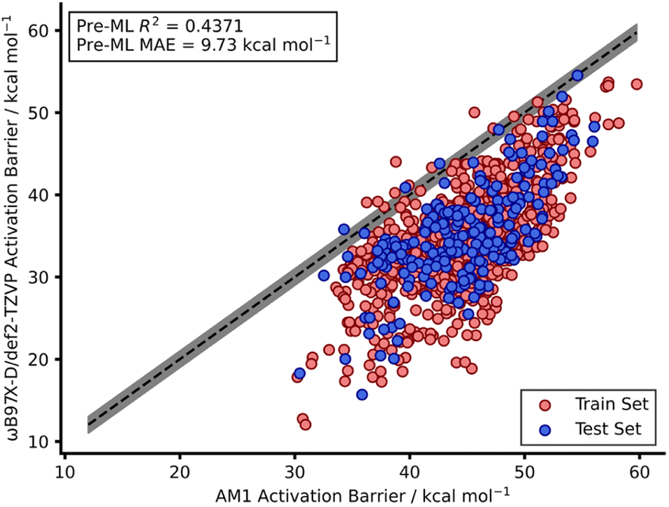Fig. 2 Scatter plot showing AM1 calculated barriers against DFT calculated barriers for the endo dataset. The dotted line shows perfect agreement between AM1 and DFT activation barriers whilst the grey region highlights the chemical accuracy threshold of 1 kcal mol⁻¹ either side of perfect agreement.

KRR and SVR have been used to address chemical-based challenges with both being used recently to achieve high accuracy barrier predictions.^5,12,70 Within this work, a variety of different models, including KRR and SVR, were tested on both the endo and exo datasets and the test MAEs and associated standard errors are presented in Fig. 3. In general, 5-fold CV training set MAEs match the test MAEs, indicating that these models are not overfit. This is also true for the NNs where overfitting was monitored with an extra validation set (see ESI,† Section 3, for more details).^14,15

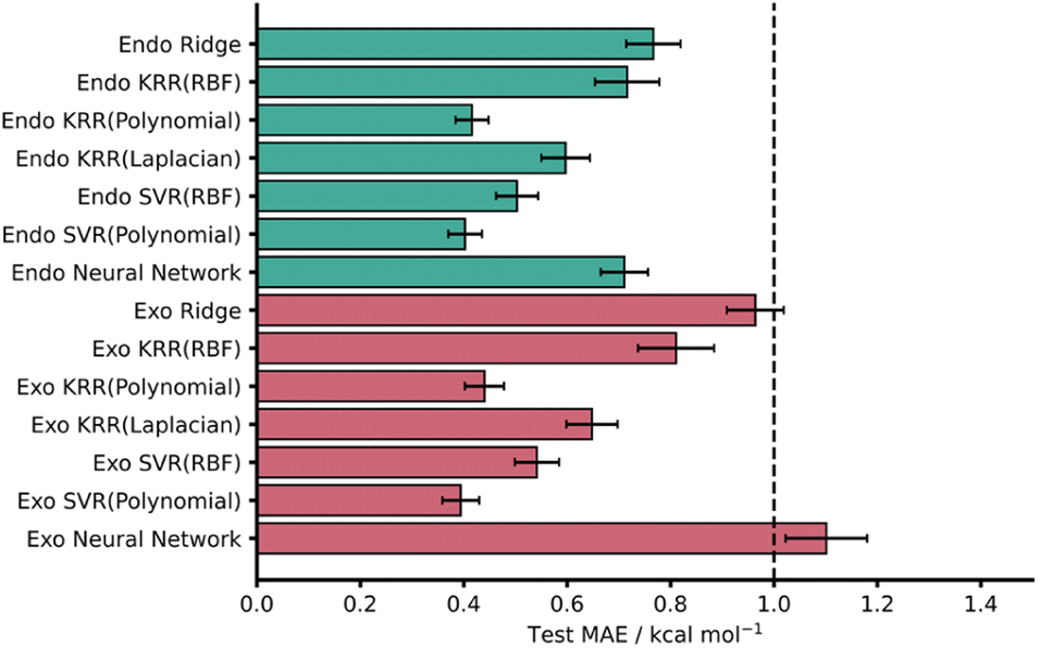Fig. 3 Test MAEs with associated standard errors for each AM1-DFT ML model (RBF = radial basis function kernel). The dotted line represents the chemical accuracy threshold of 1 kcal mol⁻¹.

Across both endo and exo datasets, most models yielded striking test set MAE results well below the chemical accuracy threshold, with the best performing models significantly lower. In line with previous work, the kernel-based models performed effectively with SVR (Polynomial) yielding the lowest MAEs for both the AM1 endo and exo datasets – test MAE values of 0.40 ± 0.03 and 0.39 ± 0.04 kcal mol⁻¹, respectively (Fig. 3).

It is worth noting that all kernels for both KRR and SVR performed comparably across both datasets and even ridge regression – which relies on linear correlations within the data – performed well, producing test MAE values below 1 kcal mol⁻¹. Furthermore, these test MAEs match very well with CV MAEs and exhibit small standard errors. Encouragingly, PM3 results were comparable to that of AM1 for all models with only ridge regression on the exo dataset missing the 1 kcal mol⁻¹ threshold (1.23 ± 0.07 kcal mol⁻¹). This is somewhat expected given the similar reported performances and underlying theory of the AM1 and PM3 methods.⁷¹ For all metrics associated with both AM1 and PM3 models see the ESI, Section 4.†

Considering the large pre-ML MAEs calculated between the AM1/PM3 and DFT barriers (Table 1), our ML approach therefore provides significant improvements in the prediction of Diels–Alder activation barriers, with accuracies well below 1 kcal mol⁻¹ for both AM1 and PM3 inputs. Not only do these results highlight the suitability of the Diels–Alder reaction to ML studies, but they also support the previously reported success of our SQM/ML approach.¹²

To rationalise the impressive model performances, we investigated the similarities between TS structures from AM1 against DFT (Fig. 4) by calculating root-mean-squared deviation of atomic positions (RMSDs) between pairs of TSs calculated at the two LoTs.⁷² In the context of molecular docking, values of <2 Å are considered accurate⁷³ and this tolerance shall also be applied here. AM1 was found to provide a strong structural approximation for this enumerated dataset of reactions relative to DFT with a mean endo and exo RMSD of 0.073 and 0.081 Å, respectively. In fact, all TS structures within the AM1 dataset fall comfortably under this 2 Å threshold by approximately an order of magnitude. Similar trends were found when this process was repeated for PM3 with DFT. When comparing AM1 and PM3 TS structures, the mean RMSDs drop further to 0.043 and 0.044 Å for endo and exo datasets, respectively, reinforcing the similarity between these two SQM methods when investigating Diels–Alder reactions. Thus, the TS structures generated via SQM calculations provide both significant mechanistic insights, given their very close approximation to the DFT TSs, and reliable data that aids the training of our highly accurate ML barrier models.

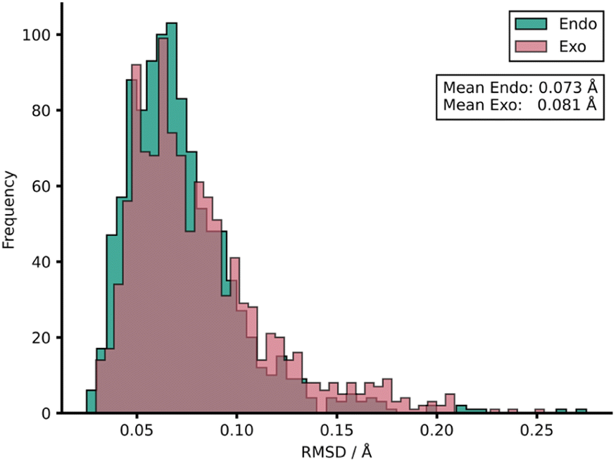Fig. 4 Distribution of RMSDs between each TS structure at AM1 and DFT for both endo and exo datasets.

As with all ML models, generalisability needs to be assessed. A model able to predict on reactions outside the immediate chemical space in which it is trained provides a more useful tool than a model hyper-specific to a particular region of chemical space. To evaluate this within our work, we utilised a leave-one-out technique focussing on leaving out reactions with specific dienes or dienophiles. Further details on the leave-one-out procedure are available in the ESI, Section 3.† Focussing on the AM1 datasets, LODiO gave a best MAE of 0.76 ± 0.11 kcal mol⁻¹ (KRR (Laplacian)), whilst the best LODpO performance was 0.61 ± 0.10 kcal mol⁻¹ (KRR (Polynomial)). Both of these results are very similar to their test MAEs. Except for Ridge and KRR (RBF), which performed consistently poorly, similarly impressive metrics were found for all other models for LODiO and LODpO predictions (Fig. 5). This implies that most models can generalise outside of the immediate chemical space for which they are trained.

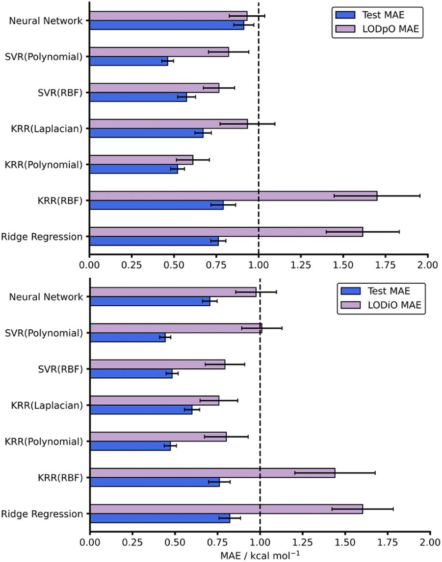Fig. 5 Test and LODpO (top) and LODiO (bottom) MAEs and associated standard errors for all models on the AM1-DFT endo dataset.

Considering both our whole dataset and our leave-one-out approaches, our NNs also performed consistently well, obtaining MAEs below 1 kcal mol⁻¹ and showing good generalisability. In addition to this strong predictive performance, they provide significant flexibility and tunability which make them an exciting tool for free energy activation barrier predictions (see hTL and dTL sections below). To evaluate these NNs further, we analysed the impact of individual features on model predictions by randomly shuffling feature values prior to test set predictions (see ESI, Section 5,† for more details). Fig. 6 shows the original AM1 endo NN test set performance together with the test performance of the features that result in the largest change in test MAE when shuffled. Unsurprisingly, the most impactful feature on model performance is the SQM barrier (ea_ts) which increases test MAE substantially to 2.83 kcal mol⁻¹. This further supports our previous work where the SQM free energy activation barriers were most important in DFT barrier predictions.¹² Some other features, such as the Mulliken⁷⁴ charges on the dienophile (atomcharges_mulliken_04_dp), also produce test predictions above the 1 kcal mol⁻¹ chemical accuracy threshold when shuffled, however this impact is not as significant as it is for the SQM barrier. Notably, the bond forming distances for both bond forming events in the TS structure (bond_forming_distance_1_ts and bond_forming_distance_2_ts) impact the predictions comparably, which can be rationalised by the concerted nature of the reactions in our dataset.

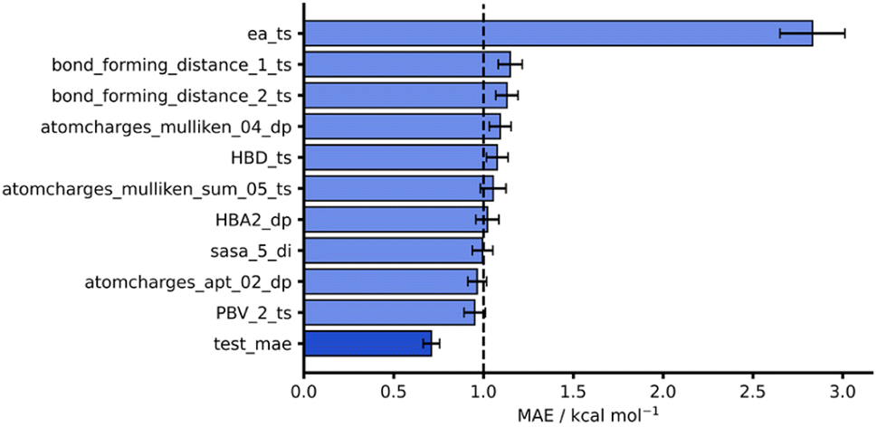Fig. 6 Feature importances for AM1 endo NN. Test MAE (dark blue) plotted with 10 highest test MAEs (light blue) achieved after feature importance analysis.

hTL

Models and results presented up until this point show that both mechanistic insight and DFT-quality free energy activation barriers can be obtained via ML from SQM structures and features at a fraction of the computational cost needed to run DFT calculations. Additionally, these models, for the most part, generalise well to leave-one-out data. As previously discussed, NNs can be adapted to make predictions outside the immediate chemical space in which they were trained by using TL. Herein, we aim to demonstrate that NN activation barrier prediction models can be adapted to make predictions for different but related reactions with minimal data requirements through hTL, and thus avoid the need to generate large data sets each time predictions are needed on a new class of reactions. To do this, we trained NNs on subsections of our full enumerated dataset and used smaller subsections as TL target datasets. Fig. 7 shows the two divisions chosen for this hTL work; models were trained on either dataset A or B, before performing hTL using target datasets α and β, respectively (see ESI,† Section 6, for more details).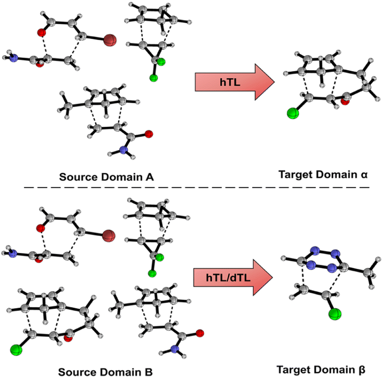

Fig. 7 Two partitions of the dataset to yield our TL targets. Source domain A contains intermolecular homo/hetero and cyclopropane Diels–Alder reactions with the target domain α containing intramolecular Diels–Alder reactions. Source domain B contains homo/hetero, inter/intra molecular, and cyclopropane Diels–Alder reactions with the target domain β containing 1,2,4,5-tetrazine Diels–Alder reactions.

The hTL targets were chosen as intramolecular Diels–Alder (α) or tetrazine reactions (β) due to their prevalence in the synthetic literature.^{43,44,50,54,55,75} Additionally, we believe these two classes of reactions should provide a suitable challenge for TL given their intramolecular and inverse electron demand natures, respectively. Due to the similarity between AM1 and PM3, all further results presented are for the AM1-DFT endo dataset only. For more hTL details see the ESI, Section 7.†

hTL to intramolecular Diels–Alder reactions (α)

This initial experiment took all intermolecular Diels–Alder reactions within the dataset (792 endo) and trained a fully tuned NN as previously outlined. The size of the hTL target dataset was 273 reactions in total, which would be considered small in the context of NNs. This dataset was split into a train, validation, and test set, totalling 174, 44 and 55 reactions, respectively. Using the intermolecular NN to predict upon the intramolecular Diels–Alder data yields a pre-hTL test MAE of 5.09 kcal mol⁻¹ which is significantly above the target accuracy of 1 kcal mol⁻¹ (Fig. 8). This result is somewhat expected given that the base NN was trained exclusively on intermolecular reactions, however it is still an improvement upon the pre-ML AM1-DFT MAE for intramolecular data of 11.31 kcal mol⁻¹ suggesting that even before hTL these models can generalise to a different reaction class to a certain degree. Currently, there are no commonly accepted criteria or workflows for the implementation of TL, however there are a few rules that are typically followed initially with consideration of both the target data size and the task-relatedness. These help to ensure the TL process chosen is suitable for the given task.²⁷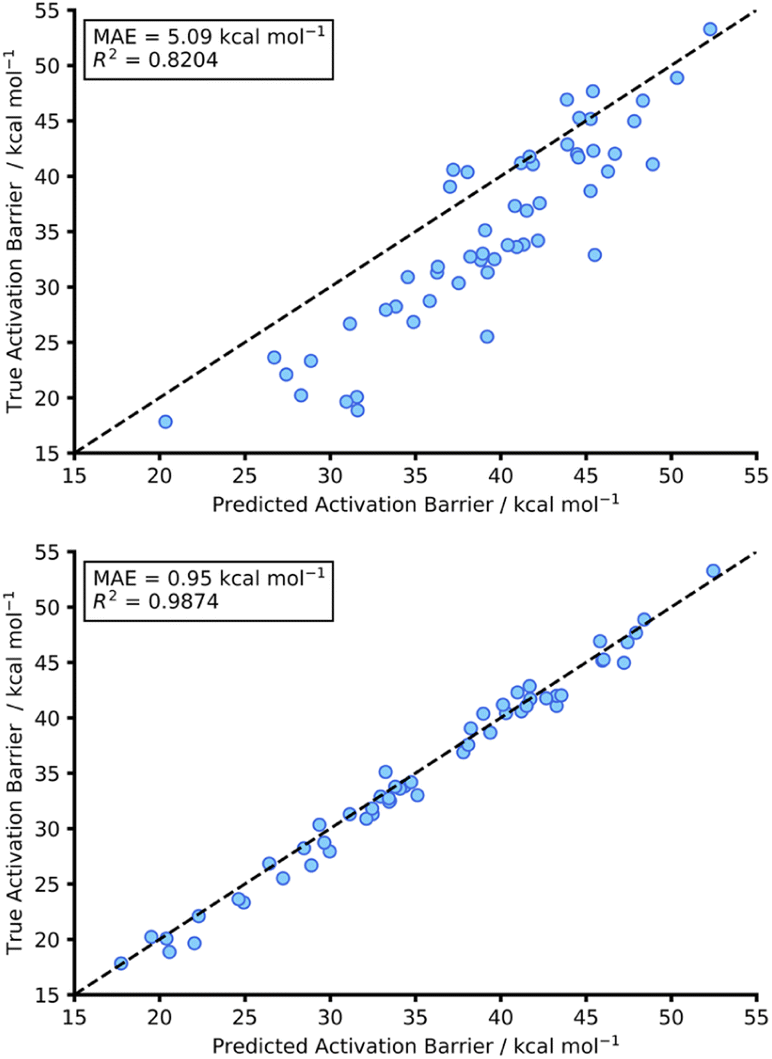

Fig. 8 Scatter graph for hTL to the intramolecular test set. The top graph shows the prediction of intramolecular data using the pre-trained NN (trained on intermolecular data) without any TL being performed. The bottom graph showing the hTL test prediction on the intramolecular after performing TL from the intermolecular data.

After employing our chosen TL process (full details are available in the ESI, Section 3†) the hTL test MAE was reduced to 0.95 kcal mol⁻¹, which not only vastly improves upon the previous prediction error from the intermolecular NN but also takes the prediction error below the chemical accuracy threshold of 1 kcal mol⁻¹, even with the limited sized training set used (Fig. 8).

To further evaluate the effect of limiting the training set size, we gradually reduced the number of hTL training datapoints and calculated MAEs averaged over several different random states (Fig. 9). This revealed that predictions near the chemical accuracy threshold for this intramolecular Diels–Alder dataset could be obtained with as few as only 70% of the hTL training points (122 reactions), whilst as few as 20% (35 reactions) of the points still produced a test MAE below 2 kcal mol⁻¹.

Fig. 9 Learning curves for hTL of source domain A to target domain α (top) and, source domain B to target domain β (bottom) using an endo base model. For all points the test MAE was obtained for three different random states and averaged. The number of datapoints in 100% of the target domains training set is 174 and 66 reactions for α and β, respectively.

Best practice dictates that given the relatively low number of intramolecular Diels–Alder datapoints available overall, and especially when the hTL training set size is reduced, much more data would need to be obtained before building a standalone intramolecular NN or risk chronically overfitting the model.²³ Instead, TL can be used in low data regimes to reduce the risk of overfitting by only retraining selected layers of a base NN, all whilst maintaining an impressive level of accuracy.³⁰

hTL to 1,2,4,5-tetrazine reactions (β)

1,2,4,5-Tetrazine Diels–Alder reactions provide an extended challenge as they are an example of an inverse electron demand Diels–Alder reaction in which aromaticity is broken. Further to this, the number of 1,2,4,5-tetrazine examples in the enumerated dataset is significantly lower (103 reactions), providing the opportunity to evaluate our hTL approach in extremely low data regimes. Following the same procedure as used for hTL from dataset A to α, a NN was trained on dataset B to give a pre-hTL prediction on β of 1.92 kcal mol⁻¹ which, akin to that of the TL results of A to α, is a vast improvement on the pre-ML AM1-DFT MAE for β of 14.54 kcal mol⁻¹. After performing hTL using the β dataset, we obtained an average test MAE of 0.86 kcal mol⁻¹ (100% training data, Fig. 9), providing another example of how TL can be utilised to achieve accurate predictions from pre-existing NNs. Analysing the impact of limited training data on hTL using dataset β reveals that strong predictive performance can be achieved with very low numbers of training points (Fig. 9); with as few as 50% of the hTL training points (33 reactions), our model yielded a 0.99 kcal mol⁻¹ hTL test MAE. This is both a significant improvement on pre-ML and pre-hTL test set predictions and acts as a useful stress test of the lower limits of TL within the barrier prediction domain. Emphasis should also be placed on just how little data is needed to provide these accurate predictions; submitting 33 SQM and DFT activation barrier calculations is a low price to pay for a model that can be used for rapid, early-stage barrier prediction in reaction discovery. Ultimately, this approach could provide crucial insights into reaction feasibility without the need for extensive high-throughput experimental or computational screening.

dTL

dTL to 1,2,4,5-tetrazine reactions (β)

Whilst we have shown that hTL allows for the prediction of free energy activation barriers in different regions of chemical space to the original model, it does not necessarily allow for transfer between different LoTs. In contrast, dTL provides the opportunity to predict in both a different chemical space and at a higher LoT, all whilst working with limited data. To evaluate the potential of dTL with our dataset, we ran calculations on target domain β (1,2,4,5-tetrazine reactions) at a higher LoT (DSD-PBEP86-D3(BJ)/def2-TZVP) and used a NN trained on source domain B to predict ωB97X-D/def2-TZVP barriers as the base model for the dTL. As with the hTL procedure to target domain β, the total number of reactions was 103. Subsequent results are for exo source domain base models, whilst endo results are available in the ESI, Section 8.†

Using the pre-trained base model NN, a pre-dTL MAE prediction on β of 10.16 kcal mol⁻¹ was obtained. Utilising the same TL process as used above, we were able to predict these barriers at the higher LoT with a significant improvement in accuracy; we obtained an average dTL MAE on target domain β of 1.23 kcal mol⁻¹ (100% training data, Fig. 10). dTL, therefore, can provide a pathway to accurate and higher LoT barrier predictions for different reactions relative to the base model NN. Furthermore, such barrier predictions can be made at a fraction of the computational cost required to calculate them with DSD-PBEP86-D3(BJ)/def2-TZVP. For example, the SQM calculations needed to make a barrier prediction using our dTL-derived NN took less than 40 seconds on a 16-core node, whereas calculating the same barrier with DSD-PBEP86-D3(BJ)/def2-TZVP took approximately 8 days on the same architecture.

Fig. 10 Learning curves for dTL of source domain B to target domain β using an exo base model. For all points the test MAE was obtained for three different random states and averaged. The number of datapoints in 100% of the target domains training set is 66 reactions.

To further evaluate the predictive ability of our dTL approach, we employed the same training percent splitting as for hTL to understand how few of these high LoT calculations would be required to make accurate predictions on target domain β. As previously seen with hTL, dTL also performs very well in low training data regimes, yielding an average test MAE approaching 1 kcal mol⁻¹ with as few as 39 training points (Fig. 10). The requirement for so few datapoints greatly minimises the computational cost associated with generating the data needed for dTL. Overall, hTL (change of reaction) performed slightly better than dTL (change of reaction and LoT), however this was expected given the greater complexity of the task associated with dTL. For full dTL results, see the ESI, Section 8.†

Comparing the TL metrics to a direct training method in these extreme low data regimes, the degree of overfitting is reduced with TL as expected. For example, with 10% training data, the difference between train and test MAEs for direct model training on source domain B and testing on target domain β was 1.00 kcal mol⁻¹, whereas the B − β dTL difference was 0.12 kcal mol⁻¹. The same trend is observed for both A − α, B − β and, [3 + 2] cycloaddition hTL when compared to direct training in low data regimes (ESI, Section 12†).

[3 + 2] cycloaddition hTL

While both the α and β target domains provide a test for our models, we wanted to further challenge our TL approach on a different reaction class. Recently, a dataset was published containing a varied set of [3 + 2] cycloadditions.⁷⁶ We enumerated 408 [3 + 2] reactions based upon this [3 + 2] cycloaddition dataset (ESI Section 6, Fig. S9†) and performed the same computational workflow previously used for our original dataset. The resulting data was then used as our new target domain utilising our source domain B (both endo and exo models) to perform hTL using the same procedure as before.

The pre-hTL MAE for the [3 + 2] AM1-DFT data was 8.26 kcal mol⁻¹. Utilising 100% of training data (326 datapoints), hTL yielded an average MAE of 0.76 kcal mol⁻¹ when predicting on the [3 + 2] test data which is substantially below the chemical accuracy threshold and a significant improvement upon the pre-hTL MAE value. Evaluating the training percentages in the same way as done previously, we obtained an MAE of less than 1 kcal mol⁻¹ with as little as 60% of the training data (196 datapoints) whilst as few as 20% of training points (65 datapoints) still produced an average MAE below 2 kcal mol⁻¹. These results highlight the power of hTL and its ability to adapt base models to make accurate predictions on different reaction classes with limited data. For full hTL results for the [3 + 2] cycloaddition dataset, see ESI, Section 7.†

Evaluating transferability

Transferability (task-relatedness) must be considered when employing TL techniques. Should the target domain be substantially different from the source, it may result in poor TL performance. For example, negative transfer, in which TL damages model performance, is a common occurrence when transferability is poor.¹⁹ Across our hTL and dTL experiments, there were no cases of negative transfer, suggesting that the source and target domains are sufficiently related, although the difference in pre-TL and TL test MAEs indicates that there is still some notable variation between the datasets. Unfortunately, task-relatedness is not easy to assess prior to dataset generation and TL, and thus development of an approach by which transferability could be quantified prior to TL would greatly aid its appropriate and effective implementation. One quantitative approach would be to measure the similarity between structures in the source and target domains.²⁷ This has been previously considered using a chemical distance measure in the form of combining fingerprints and subgraphs⁷⁷ in addition to using Tanimoto coefficients based on molecular fingerprints.⁷⁸ Thus, in an attempt to assess the transferability from our source to our target domains, we utilised either Tanimoto or Dice similarities on Morgan fingerprints of each SQM TS structure within the source domain and hTL target domain. Tanimoto and Dice similarities were then calculated for every structure in the source domain against every structure in the target domain (A to α and B to β). The mean was taken over these similarities to provide a metric used to evaluate the transferability of predictions to datasets α and β (Fig. 11 and 12, see ESI, Section 11,† for full similarity procedure). The use of Morgan fingerprints in this way could allow an initial assessment of transferability between source and target domains prior to DFT target domain data generation with only the need to run rapid and inexpensive SQM calculations. With Tanimoto and Dice similarity metrics, a value of 1 would equate to the same structure.

Fig. 11 Source domain A to target domain α mean endo TS structure Tanimoto (top) and Dice (bottom) similarity obtained from Morgan fingerprints of the source and target domains.

Fig. 12 Source domain B to target domain β mean endo TS structure Tanimoto (top) and Dice (bottom) similarity obtained from Morgan fingerprints of the source and target domains.

Across both α and β hTL comparisons, Dice and Tanimoto similarities are extremely low. This reinforces the power of our hTL approach given the impressive prediction accuracies seen in these low data regimes, even when there are substantial differences between source and domain structures.

Comparing mean Tanimoto and Dice similarities for α and β is challenging due to both having marginally different source domain sizes. Nevertheless, both similarity metrics indicate that the β dataset is less similar to its respective source domain (B). As shown earlier, hTL provides high accuracy predictions in low data regimes for α and β. The higher similarity across both metrics for dataset α would suggest higher transferability, however this is not seen within the hTL results; instead, predictions below 1 kcal mol⁻¹ can be obtained on dataset β with substantially fewer reactions than needed for dataset α (Fig. 9). This implies that for our Diels–Alder datasets, Morgan fingerprints do not necessarily provide a good indicator of transferability from source to target domain.

A feature vector similarity approach was also considered, which yielded the same trend observed when utilising the fingerprint approach outlined previously. Full information on this can be found in the ESI, Section 11.† Alternatively, more advanced transferability metrics have very recently been reported within computer science.^79,80 Thus, the concept of transferability for TL within chemistry is an area which would benefit from further research that could yield metrics capable of quantifying the likely success of TL prior to target dataset generation and model retraining.

Conclusions

In this work we have developed ML models that can predict DFT-quality free energy activation barriers for a broad range of Diels–Alder reactions with test MAEs significantly below the chemical accuracy threshold of 1 kcal mol⁻¹ using rapidly generated SQM features. The ML models generalise well, and predictions are available in a fraction of the time required to calculate the barriers with DFT (seconds instead of hours). Coupled with this accurate barrier prediction, both SQM methods tested provide TS structures in excellent agreement with those calculated with DFT, thus yielding rapid, high-quality mechanistic insight for Diels–Alder reactions. We also report the first examples of hTL and dTL applied to reaction barrier prediction in which pre-trained NNs are adapted to other reaction classes (hTL and dTL) or other LoTs (dTL), both in extremely low data regimes. We observe prediction errors below 1 kcal mol⁻¹ with as few as 33 and 39 training points via hTL and dTL, respectively. We hope that such low data requirements could provide a pathway for pre-trained NNs to be integrated into synthesis projects; by running just a few dozen calculations and utilising TL, NNs could be adapted to make predictions that inform chemists about the feasibility of a series of new reactions before any experiments need to be performed. We recommend further work in this area to establish the limits of hTL and dTL and also metrics capable of quantifying the likely success of TL in the context of reaction barrier prediction.

Data availability

Gaussian 16 computed output files and code from this work is available in Dataset for “Machine learning reaction barriers in low data regimes: a horizontal and diagonal transfer learning approach” in the University of Bath Research Data Archive (accessible at: https://doi.org/10.15125/BATH-01229).

Author contributions

S. G. E. performed calculations and ML analysis, M. N. G., S. T., and D. B. devised and supervised the work, and E. H. E. F. provided early code examples and support with calculations. The manuscript was written through contributions from all authors.

Conflicts of interest

There are no conflicts of interest to declare.

Acknowledgements

The authors gratefully acknowledge the University of Bath's Research Computing Group (https://doi.org/10.15125/b6cd-s854) for their support in this work; this research made use of both the Balena and Anatra High Performance Computing (HPC) service at the University of Bath. The authors thank the EPSRC (EP/W003724/1, EP/V519637/1 and EP/R513155/1), the University of Bath and AstraZeneca for funding.

Notes and references

1. D. H. Ess and K. N. Houk, J. Phys. Chem. A, 2005, 109, 9542–9553.
2. Y. Zhao and D. G. Truhlar, J. Chem. Theory Comput., 2011, 7, 669–676.
3. Y. H. Lam, M. N. Grayson, M. C. Holland, A. Simon and K. N. Houk, Acc. Chem. Res., 2016, 49, 750–762.
4. K. Hansen, F. Biegler, R. Ramakrishnan, W. Pronobis, O. A. von Lilienfeld, K.-R. Müller and A. Tkatchenko, J. Phys. Chem. Lett., 2015, 6, 2326–2331.
5. M. Bragato, G. F. von Rudorff and O. A. von Lilienfeld, Chem. Sci., 2020, 11, 11859–11868.
6. M. Döntgen, Y. Fenard and K. A. Heufer, J. Chem. Inf. Model., 2020, 60, 5928–5931.
7. P. Friederich, G. Dos Passos Gomes, R. De Bin, A. Aspuru-Guzik and D. Balcells, Chem. Sci., 2020, 11, 4584–4601.
8. F. Palazzesi, M. R. Hermann, M. A. Grundl, A. Pautsch, D. Seeliger, C. S. Tautermann and A. Weber, J. Chem. Inf. Model., 2020, 60, 2915–2923.
9. C. A. Grambow, L. Pattanaik and W. H. Green, J. Phys. Chem. Lett., 2020, 11, 2992–2997.
10. S. Choi, Y. Kim, J. W. Kim, Z. Kim and W. Y. Kim, Chem.–Eur. J., 2018, 24, 12354–12358.
11. S. Vargas, M. R. Hennefarth, Z. Liu and A. N. Alexandrova, J. Chem. Theory Comput., 2021, 17, 6203–6213.
12. E. H. E. Farrar and M. N. Grayson, Chem. Sci., 2022, 13, 7594–7603.
13. T. Lewis-Atwell, P. A. Townsend and M. N. Grayson, Wiley Interdiscip. Rev.: Comput. Mol. Sci., 2022, 12, e1593.
14. X. García-Andrade, P. García Tahoces, J. Pérez-Ríos and E. Martínez Núñez, J. Phys. Chem. A, 2023, 127, 2274–2283.
15. K. A. Peterson, D. Feller and D. A. Dixon, Theor. Chem. Acc., 2012, 131, 1079.
16. K. N. Houk and F. Liu, Acc. Chem. Res., 2017, 50, 539–543.
17. K. Burke, J. Chem. Phys., 2012, 136, 1–8.
18. S. J. Pan and Q. Yang, IEEE Trans. Knowl. Data Eng., 2010, 22, 1345–1359.
19. K. Weiss, T. M. Khoshgoftaar and D. D. Wang, J. Big Data, 2016, 3, 1–40.
20. F. Zhuang, Z. Qi, K. Duan, D. Xi, Y. Zhu, H. Zhu, H. Xiong and Q. He, Proc. IEEE, 2021, 109, 43–76.
21. M. L. Hutchinson, E. Antono, B. M. Gibbons, S. Paradiso, J. Ling and B. Meredig, arXiv, 2017, preprint, arXiv:1711.05099,  DOI:10.48550/arXiv.1711.05099.
22. C. A. Grambow, Y.-P. Li and W. H. Green, J. Phys. Chem. A, 2019, 123, 5826–5835.
23. T. Dietterich, ACM Comput. Surv., 1995, 27, 326–327.
24. D. M. Hawkins, J. Chem. Inf. Comput. Sci., 2004, 44, 1–12.
25. S. J. Nowlan and G. E. Hinton, Neural Comput., 1992, 4, 473–493.
26. L. Huang and C. Ling, J. Chem. Inf. Model., 2021, 61, 4200–4209.
27. C. Cai, S. Wang, Y. Xu, W. Zhang, K. Tang, Q. Ouyang, L. Lai and J. Pei, J. Med. Chem., 2020, 63, 8683–8694.
28. S. Singh and R. B. Sunoj, Digital Discovery, 2022, 1, 303–312.
29. F. H. Vermeire and W. H. Green, Chem. Eng. J., 2021, 418, 129307.
30. J. S. Smith, B. T. Nebgen, R. Zubatyuk, N. Lubbers, C. Devereux, K. Barros, S. Tretiak, O. Isayev and A. E. Roitberg, Nat. Commun., 2019, 10, 1–8.
31. Y. Zhang, L. Wang, X. Wang, C. Zhang, J. Ge, J. Tang, A. Su and H. Duan, Org. Chem. Front., 2021, 8, 1415–1423.
32. G. Pesciullesi, P. Schwaller, T. Laino and J. L. Reymond, Nat. Commun., 2020, 11, 1–8.
33. K. A. Spiekermann, L. Pattanaik and W. H. Green, J. Phys. Chem. A, 2022, 126, 3976–3986.
34. J.-A. Funel and S. Abele, Angew. Chem., Int. Ed., 2013, 52, 3822–3863.
35. B. Jursic and Z. Zdravkovski, J. Chem. Soc., Perkin Trans. 1, 1995, 9, 1223–1226.
36. K. N. Houk, F. Liu, Z. Yang and J. I. Seeman, Angew. Chem., Int. Ed., 2021, 60, 12660–12681.
37. F. Liu, R. S. Paton, S. Kim, Y. Liang and K. N. Houk, J. Am. Chem. Soc., 2013, 135, 15642–15649.
38. I. Fernández and F. M. Bickelhaupt, Chem.–Asian J., 2016, 11, 3297–3304.
39. B. J. Levandowski, L. Zou and K. N. Houk, J. Org. Chem., 2018, 83, 14658–14666.
40. B. J. Levandowski and K. N. Houk, J. Org. Chem., 2015, 80, 3530–3537.
41. W. Beker, E. P. Gajewska, T. Badowski and B. A. Grzybowski, Angew. Chem., Int. Ed., 2019, 58, 4515–4519.
42. T. A. Young, T. Johnston-Wood, H. Zhang and F. Duarte, Phys. Chem. Chem. Phys., 2022, 24, 20820–20827.
43. L. M. Harwood, G. Jones, J. Pickard, R. M. Thomas and D. Watkin, Tetrahedron Lett., 1988, 29, 5825–5828.
44. L. M. Harwood, S. A. Leeming, N. S. Isaacs, G. Jones, J. Pickard, R. M. Thomas and D. Watkin, Tetrahedron Lett., 1988, 29, 5017–5020.
45. R. Gordillo and K. N. Houk, J. Am. Chem. Soc., 2006, 128, 3543–3553.
46. B. J. Levandowski and K. N. Houk, J. Am. Chem. Soc., 2016, 138, 16731–16736.
47. P. Binger, P. Wedemann, R. Goddard and U. H. Brinker, J. Org. Chem., 1996, 61, 6462–6464.
48. L. A. Fisher, N. J. Smith and J. M. Fox, J. Org. Chem., 2013, 78, 3342–3348.
49. F. Liu, R. S. Paton, S. Kim, Y. Liang and K. N. Houk, J. Am. Chem. Soc., 2013, 135, 15642–15649.
50. R. Ukis and C. Schneider, J. Org. Chem., 2019, 84, 7175–7188.
51. V. Eschenbrenner-Lux, K. Kumar and H. Waldmann, Angew. Chem., Int. Ed., 2014, 53, 11146–11157.
52. D. V. Osipov, V. A. Osyanin, G. D. Khaysanova, E. R. Masterova, P. E. Krasnikov and Y. N. Klimochkin, J. Org. Chem., 2018, 83, 4775–4785.
53. S. N. Pieniazek and K. N. Houk, Angew. Chem., Int. Ed., 2006, 45, 1442–1445.
54. N. K. Devaraj, R. Weissleder and S. A. Hilderbrand, Bioconjugate Chem., 2008, 19, 2297–2299.
55. F. Liu, Y. Liang and K. N. Houk, J. Am. Chem. Soc., 2014, 136, 11483–11493.
56. Maestro Schrödinger, Schrödinger Release 2018-2, LLC, New York, 2018.
57. MacroModel Schrödinger, Schrödinger Release 2018-2, 2018.
58. F. Mohamadi, N. G. J. Richards, W. C. Guida, R. Liskamp, M. Lipton, C. Caufield, G. Chang, T. Hendrickson and W. C. Still, J. Comput. Chem., 1990, 11, 440–467.
59. K. Roos, C. Wu, W. Damm, M. Reboul, J. M. Stevenson, C. Lu, M. K. Dahlgren, S. Mondal, W. Chen, L. Wang, R. Abel, R. A. Friesner and E. D. Harder, J. Chem. Theory Comput., 2019, 15, 1863–1874.
60. M. J. S. Dewar, E. G. Zoebisch, E. F. Healy and J. J. P. Stewart, J. Am. Chem. Soc., 1985, 107, 3902–3909.
61. J. J. P. Stewart, J. Comput. Chem., 1989, 10, 221–264.
62. J.-D. Chai and M. Head-Gordon, Phys. Chem. Chem. Phys., 2008, 10, 6615.
63. F. Weigend and R. Ahlrichs, Phys. Chem. Chem. Phys., 2005, 7, 3297–3305.
64. M. J. Frisch, G. W. Trucks, H. B. Schlegel, G. E. Scuseria, M. A. Robb, J. R. Cheeseman, G. Scalmani, V. Barone, B. Mennucci, G. A. Petersson, H. Nakatsuji, M. Caricato, X. Li, H. P. Hratchian, A. F. Izmaylov, J. Bloino, J. Zheng, J. L. Sonnenberg, M. Hada, M. Ehara, K. Toyota, R. Fukuda, J. Hasegawa, M. Ishida, T. Nakajima, Y. Honda, O. Kitao, H. Nakai, T. Vreven, J. A. Montgomery, J. E. Peralta, F. Ogliaro, M. Bearpark, J. J. Heyd, E. Brothers, K. N. Kudin, V. N. Staroverov, R. Kobayashi, J. Normand, K. Raghavachari, J. C. A. Rendell, S. Burant, S. Iyengar, J. Tomasi, M. Cossi, N. Rega, J. M. Millam, M. Klene, J. E. Knox, J. B. Cross, V. Bakken, C. Adamo, J. Jaramillo, R. Gomperts, R. E. Stratmann, O. Yazyev, A. J. Austin, R. Cammi, C. Pomelli, J. W. Ochterski, R. L. Martin, K. Morokuma, V. G. Zakrzewski, G. A. Voth, P. Salvador, J. J. Dannenberg, S. Dapprich, A. D. Daniels, O. Farkas, J. B. Foresman, J. V. Ortiz, J. Cioslowski and D. J. Fox, Gaussian 16, Revision A.03, Gaussian, Inc., Wallingford, CT, 2016.
65. M. J. Frisch, G. W. Trucks, H. B. Schlegel, G. E. Scuseria, M. A. Robb, J. R. Cheeseman, G. Scalmani, V. Barone, B. Mennucci, G. A. Petersson, H. Nakatsuji, M. Caricato, X. Li, H. P. Hratchian, A. F. Izmaylov, J. Bloino, J. Zheng, J. L. Sonnenberg, M. Hada, M. Ehara, K. Toyota, R. Fukuda, J. Hasegawa, M. Ishida, T. Nakajima, Y. Honda, O. Kitao, H. Nakai, T. Vreven, J. A. Montgomery, J. E. Peralta, F. Ogliaro, M. Bearpark, J. J. Heyd, E. Brothers, K. N. Kudin, V. N. Staroverov, R. Kobayashi, J. Normand, K. Raghavachari, J. C. A. Rendell, S. Burant, S. Iyengar, J. Tomasi, M. Cossi, N. Rega, J. M. Millam, M. Klene, J. E. Knox, J. B. Cross, V. Bakken, C. Adamo, J. Jaramillo, R. Gomperts, R. E. Stratmann, O. Yazyev, A. J. Austin, R. Cammi, C. Pomelli, J. W. Ochterski, R. L. Martin, K. Morokuma, V. G. Zakrzewski, G. A. Voth, P. Salvador, J. J. Dannenberg, S. Dapprich, A. D. Daniels, O. Farkas, J. B. Foresman, J. V. Ortiz, J. Cioslowski and D. J. Fox, Gaussian 16, Revision C.01, Gaussian, Inc., Wallingford, CT, 2016.
66. S. Kozuch and J. M. L. Martin, Phys. Chem. Chem. Phys., 2011, 13, 20104–20107.
67. G. Luchini, J. v Alegre-Requena, I. Funes-Ardoiz and R. S. Paton, F1000Research, 2020, 9, 291.
68. F. Pedregosa, V. Michel, O. Grisel, M. Blondel, P. Prettenhofer, R. Weiss, J. Vanderplas, D. Cournapeau, F. Pedregosa, G. Varoquaux, A. Gramfort, B. Thirion, O. Grisel, V. Dubourg, A. Passos, M. Brucher, M. Perrot and É. Duchesnay, J. Mach. Learn. Res., 2011, 12, 2825–2830.
69. M. Abadi, A. Agarwal, B. Paul, E. Brevdo, Z. Chen, C. Craig, G. S. Corrado, A. Davis, J. Dean, M. Devin, S. Ghemawat, I. Goodfellow, A. Harp, G. Irving, M. Isard, R. Jozefowicz, Y. Jia, L. Kaiser, M. Kudlur, J. Levenberg, D. Mané, M. Schuster, R. Monga, S. Moore, D. Murray, C. Olah, J. Shlens, B. Steiner, I. Sutskever, K. Talwar, P. Tucker, V. Vanhoucke, V. Vasudevan, F. Viégas, O. Vinyals, P. Warden, M. Wattenberg, M. Wicke, Y. Yu and X. Zheng, TensorFlow: Large-scale machine learning on heterogeneous systems, 2015.
70. K. Jorner, T. Brinck, P.-O. Norrby and D. Buttar, Chem. Sci., 2021, 12, 1163–1175.
71. M. J. S. Dewar, E. F. Healy, A. J. Holder and Y. C Yuan, J. Comput. Chem., 1990, 11, 541–542.
72. D. L. Theobald, Acta Crystallogr., Sect. A: Found. Crystallogr., 2005, 61, 478–480.
73. H. Gohlke, M. Hendlich and G. Klebe, J. Mol. Biol., 2000, 295, 337–356.
74. R. S. Mulliken, J. Chem. Phys., 2004, 23, 1833.
75. Y. T. Lin and K. N. Houk, Tetrahedron Lett., 1985, 26, 2517–2520.
76. T. Stuyver, K. Jorner and C. W. Coley, Sci. Data, 2023, 10, 1–14.
77. T. Girschick, U. Ruckert and S. Kramer, Comput. J., 2013, 56, 274–288.
78. S. Kearnes, B. Goldman and V. Pande, arXiv, 2016, preprint, arXiv:1606.08793v3,  DOI:10.48550/arXiv.1606.08793.
79. C. V. Nguyen, T. Hassner, M. Seeger and C. Archambeau, arXiv, 2020, preprint, arXiv:2002.12462,  DOI:10.48550/arXiv.2002.12462.
80. Y. Tan, Y. Li and S. L. Huang, arXiv, 2021, preprint, arXiv:2103.13843,  DOI:10.48550/arXiv.2103.13843.

---

Footnote

† Electronic supplementary information (ESI) available: Additional details on generation of SQM and DFT data, ML features, ML/TL analysis and model performance evaluation. See DOI: https://doi.org/10.1039/d3dd00085k

---