
 Open Access Article
 This Open Access Article is licensed under a Creative Commons Attribution-Non Commercial 3.0 Unported Licence
A scientific machine learning framework to understand flash graphene synthesis†
Kianoosh
Sattari
 a,
Lucas
Eddy
bc,
Jacob L.
Beckham
b,
Kevin M.
Wyss
b,
Richard
Byfield
a,
Long
Qian
b,
James M.
Tour
*bde and
Jian
Lin
*a
a,
Lucas
Eddy
bc,
Jacob L.
Beckham
b,
Kevin M.
Wyss
b,
Richard
Byfield
a,
Long
Qian
b,
James M.
Tour
*bde and
Jian
Lin
*a
aDepartment of Mechanical and Aerospace Engineering, University of Missouri, Columbia, Missouri 65211, USA. E-mail: linjian@missouri.edu; tour@rice.edu
bDepartment of Chemistry, Rice University, 6100 Main Street, Houston, Texas 77005, USA
cApplied Physics Program and Smalley-Curl Institute, Rice University, 6100 Main Street, Houston, Texas 77005, USA
dDepartment of Materials Science and NanoEngineering, Rice University, 6100 Main Street, Houston, Texas 77005, USA
eDepartment of Computer Science and Engineering, NanoCarbon Center, Welch Institute for Advanced Materials, Rice University, 6100 Main Street, Houston, Texas 77005, USA
First published on 18th July 2023
Abstract
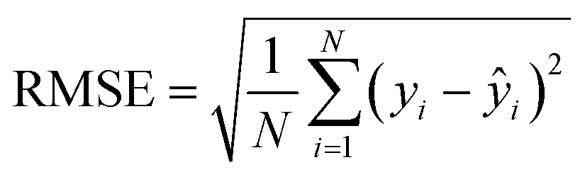
Flash Joule heating (FJH) is a far-from-equilibrium (FFE) processing method for converting low-value carbon-based materials to flash graphene (FG). Despite its promises in scalability and performance, attempts to explore the reaction mechanism have been limited due to the complexities involved in the FFE process. Data-driven machine learning (ML) models effectively account for the complexities, but the model training requires a considerable amount of experimental data. To tackle this challenge, we constructed a scientific ML (SML) framework trained by using both direct processing variables and indirect, physics-informed variables to predict the FG yield. The indirect variables include current-derived features (final current, maximum current, and charge density) predicted from the proxy ML models and reaction temperatures simulated from multi-physics modeling. With the combined indirect features, the final ML model achieves an average R2 score of 0.81 ± 0.05 and an average RMSE of 12.1% ± 2.0% in predicting the FG yield, which is significantly higher than the model trained without them (R2 of 0.73 ± 0.05 and an RMSE of 14.3% ± 2.0%). Feature importance analysis validates the key roles of these indirect features in determining the reaction outcome. These results illustrate the promise of this SML to elucidate FFE material synthesis outcomes, thus paving a new avenue to processing other datasets from the materials systems involving the same or different FFE processes.
1 Introduction
Despite the vast applications of graphene, scalable synthesis of graphene remains a tremendous challenge. Among the reported various types of processing methods,1,2 flash Joule heating (FJH) was introduced in 2020 to synthesize gram-scale graphene from different carbon feedstocks,3 such as carbon black (CB), metallurgical coke (MC), and waste plastics.4,5 FJH is an electrothermal process in which Joule heating, driven by capacitors with very high discharge rates, affords gross morphological changes.2 The generated high temperature (>3000 K) breaks the chemical bonds and reorganizes the carbon atoms into thermodynamically stable sp2-hybridized graphene sheets.2 Because the whole process is finished in a sub-second scale, the generated graphene sheets form a metastable state, namely turbostratic graphene, which was termed as flash graphene (FG).2 Such FG remains highly anisotropic in interlayer arrangements.3 This feature makes it highly dispersible in solvents and a superior additive for high-performance composites.3,6The scalability of the FJH makes it a promising method for synthesizing the FG, but many unknowns remain in this far-from-equilibrium (FFE) process,7 making it difficult to establish a processing–property relationship.8,9 Recently emerged data-driven modeling may provide an alternative solution. In the past several years, some models have been demonstrated to be powerful for tackling a variety of challenges including guiding materials synthesis.10–14 Furthermore, we recently constructed pure data-driven models to discover the parameters that controlled the FG yield.15 However, despite reaching an impressive accuracy in predicting the FG yield, the model performance depended on the current parameters measured from the reactions. These intermediate parameters were therefore unavailable as input parameters for prediction if the experiments had not yet been performed. As a result, one cannot apply such models to accurately predict the reaction outcome from a new set of direct input parameters such as voltage, pulse duration, and capacitance prior to experimentation, which makes them impractical for real applications. Thus, developing an ML framework that only uses the direct, controllable experimental parameters to accurately predict reaction outcomes of FJH remains a challenge.
Normally, a data-driven ML model is a “black-box”, lacking interpretability in mapping the relationship of the input and output. Moreover, model training requires considerable amount of data, a crucial aspect that has been a bottleneck for many materials processing methods such as FJH for FG synthesis.16,17 In contrast, physics-based models can learn the relationships of the input and output space. Although these models are highly interpretable, they are often difficult to be constructed from complex systems due to a lack of information about the behavior of the system. Thus, the approximations are needed to construct physics-based modeling while they can result in inherent model bias. Therefore, hybrid models that combine data-driven and physics-based modeling can be beneficial in successful model training with limited experimental data while offering high explainability.18–20 These models can be constructed by modifying the cost functions within data-driven ML models. This modification can adjust the model to obey the outputs of the physics-based models. Daw et al. designed a physics-guided neural networks (PGNNs) framework that leveraged the output of the physics-based model and observational features by modifying the loss function of the neural network.21 Raissi et al. introduced physics-informed neural networks (PINNs) that obeyed physics laws described by partial differential equations.22 The additional information gained from the physical laws can train the networks with much less data than needed in pure ML models, thus broadening the applications where data generation is costly.17 Rabczuk's group constructed deep neural networks (DNNs) to approximate partial differential equations for predictions of materials properties.23,24 They included the system energy in the loss function of the models. However, in the FJH process, they are not practical since there are no defined physical rules that can well describe the FFE reactions. Another method of including physics laws into the ML models is to extract physics-informed features from the experiments or theory, which are used as the model input to boost the prediction accuracy.20,25 Sun et al. synergized the indirect physics-informed descriptors with other direct variables in the ML framework to develop materials with superior properties.26 To develop thermo-responsive materials, Huang et al. developed a framework where ML models were informed with physicochemical descriptors derived from quantum chemistry calculation.27 Such physics-based descriptors can serve as the indirect input features to introduce partial physical information to the ML framework.
To better understand the FJH process for FG synthesis, herein, we demonstrate a scientific machine learning (SML) framework that is trained with both direct experimental parameters and indirect physics-informed ones. The goal is to predict the yield of FG. To estimate the reaction temperature from the direct experimental parameters (such as pulse time, voltage, capacitance, and physical information of the input materials), we performed an electrical–thermal multi-physics simulation by COMSOL. Other important indirect features such as the current parameters of final current, maximum current, and charge density were predicted from the proxy ML models. We hypothesize that these current parameters are correlated with the direct experimental parameters and physical properties of the starting materials. To validate this hypothesis, three proxy ML models were trained on these direct parameters to predict those intermediate parameters for a new experiment. In this way, the final ML model does not rely on any intermediate information to predict the reaction outcome if given a new set of direct experimental parameters. Thus, the resulting SML framework is generalizable and needs only limited training samples.21
This SML framework has three advantages over our previously reported ML model.15 First, the models are able to make predictions about the reaction outcome without using any intermediate parameters. This facilitates the use of our prediction model in a model-based optimization algorithm to optimize the FG yield in just a few iterations. Second, the physics-informed descriptors bring additional information to the model, making the black-box ML models more generalizable and accurate in addition to improving the model interpretability. Third, a general methodology of using separate ML models to predict unknown, intermediate reaction parameters from known direct ones is proposed to solve the challenge of lacking enough input features, particularly related to experiments. Thus, such an approach can be readily applied to other materials processed by the same or different methods. For instance, our developed framework could be employed to predict the yield of the precious metals recovered from electronic wastes as well as the removing efficiency of hazardous heavy metals from them by using the same FJH process.28 Furthermore, the framework holds a potential for guiding structure- and phase-controlled synthesis of inorganic nanocrystals through ultrafast FJH.29,30 It can be done by some exploratory studies to identify the specific important features and collect more experimental data from the new reactions.
2 Results and discussion
This work used a dataset consisting of 173 separate FJH reactions reported in our previous work.15 The starting materials were carbon black (CB), metallurgical coke (MC), plastic waste-derived pyrolysis ash (PA), and waste tire-based carbon black (TCB). The structures of the final products were assessed by wide-area Raman mapping. We applied custom-written scripts to analyze the collected Raman spectra, which were used to estimate the FG yield. The high-throughput mapping assay guarantees the comprehensive representation of the overall property of each sample. In the following sections, we first analyze the dataset and explain how to quantify the FG yield. We then elaborate the SML framework. Lastly, we present the model performance in predicting the FG yield.2.1 Analysis of input and output data
Raman spectroscopy has been considered a powerful technique for characterization of carbon structures.31,32Fig. 1a shows Raman spectra of amorphous carbon and synthesized FG. The spectrum of amorphous carbon shows two main peaks: D-band at ∼1350 cm−1 and G-band at ∼1600 cm−1. The Raman spectrum of FG has a G-peak at ∼1580 cm−1 and a 2D band at ∼2700 cm−1. The existence of this 2D band suggests formation of a graphitic lattice.32 This resonance-enhanced single-Lorentzian 2D band has a narrow full-width at half-maximum (FWHM) of ∼16 cm−1. The I2D/IG peak intensity ratio reaches up to 17. Both of them suggest good FG crystallinity.33 From each sample, we collected 100 Raman spectra, which was then averaged to mitigate the variance in the collected individual spectrum. Then, the FG yield can be calculated from these averaged spectra.15Fig. 1b–e represent the histograms and statistics distribution of the collected samples for each reaction of all the 173 reactions. Specifically, Fig. 1b shows the distribution of average I2D/IG with a mean of 0.66 and a standard deviation of 0.17. Fig. 1c represents a histogram of average ID/IG with a mean of 0.54 and a standard deviation of 0.14. Fig. 1d represents the average FWHM of the 2D band with a mean of 43.88 cm−1 and a standard deviation of 11.55 cm−1. Finally, Fig. 1e shows a histogram of the FG yield with a mean of 54% and a standard deviation of 27%. Fig. S1† shows the yield distribution of the FG synthesized from the four starting materials.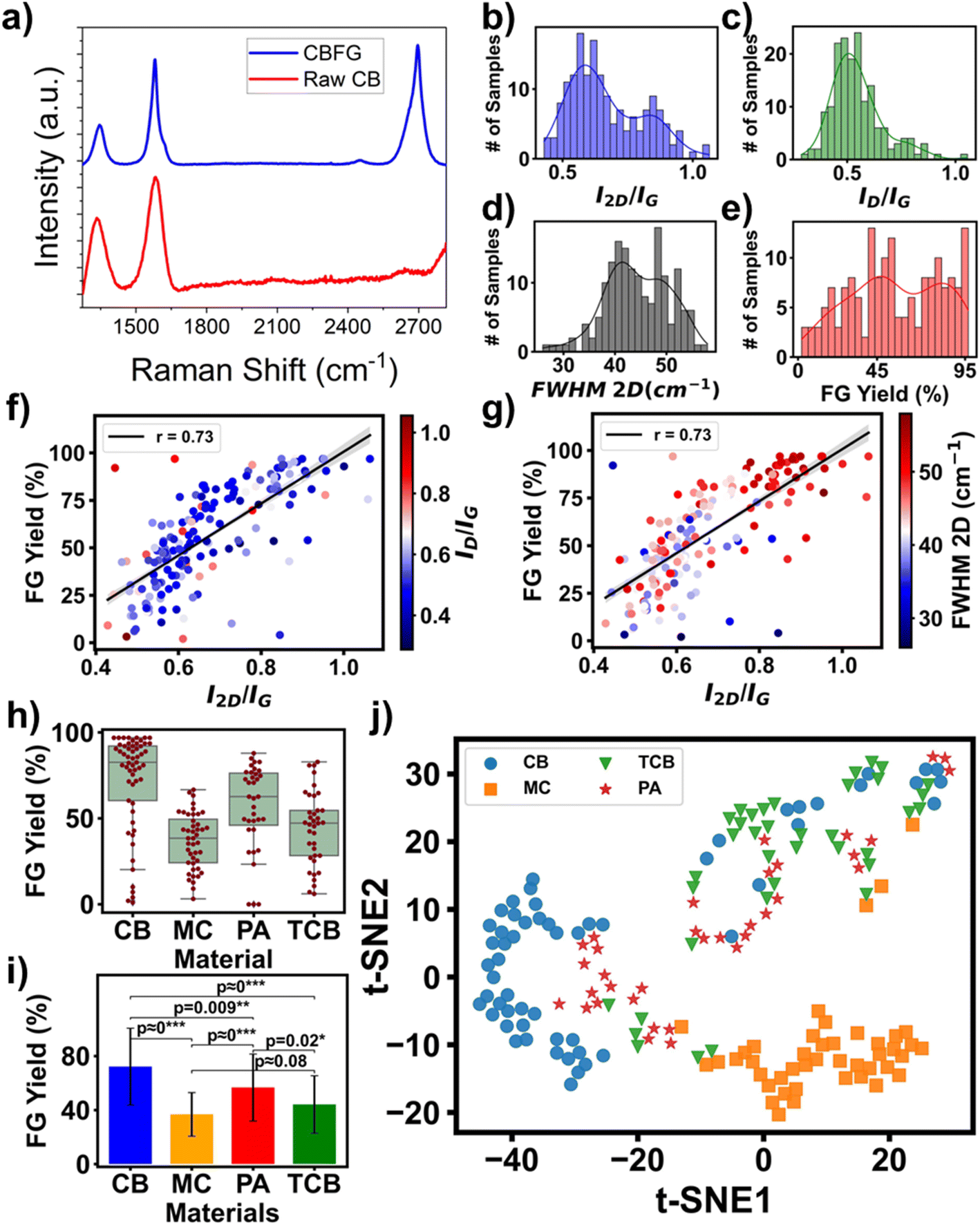 | ||
| Fig. 1 (a) Raman spectra of flash graphene (FG) synthesized from carbon black and amorphous carbon. (b–e) Statistical distribution of I2D/IG (b), ID/IG (c), FWHM of the 2D band (d), and FG yield (e). Distribution of I2D/IGversus FG yield in correlation with (f) ID/IG and (g) FWHM. (h) Distribution of FG yield synthesized from four starting materials. (i) Statistical comparison on the mean FG yield from four starting materials. (***), (**), and (*) show significant differences at 0.001, 0.01, and 0.05 levels, respectively. (j) t-SNE plots of features in correlation with the four starting materials. The features include resistance drop, voltage drop, maximum current, charge density, I2D/IG, ID/IG, FWHM, and reaction yield. | ||
Fig. 1f and g represent high correlation of I2D/IG with the FG yield, showing a Pearson's r value of 0.73. Fig. 1f shows little dependence of the FG yield on ID/IG, while the value of FWHM can well distinguish the samples with a high FG yield (Fig. 1g). Most samples have average FWHM values of >40 cm−1 and I2D/IG > 0.75. We also analyzed the FG yield from different starting materials. As illustrated in Fig. 1h, the highest FG yield of 72% and the lowest yield of 37% were obtained for CB and MC, respectively. Fig. 1i shows the statistical comparison of the FG yield obtained from the four starting materials. Except for MC versus TCB, all other two-way comparisons show significant differences at a set 0.05 significance level.
We hypothesized that the measured parameters including resistant drop, voltage drop, final current, maximum current, charge density, I2D/IG, ID/IG, FWHM, and reaction yield would depend on the starting material. To test the hypothesis, we applied t-distributed stochastic neighbor embedding (t-SNE),34 a non-linear dimension reduction method, to project all of them in 2D space (Fig. 1j). This analysis shows that those obtained from MC and CB are clustered and separated from the others, which indicates that there do exist combination of the parameters for achieving the highest FG yield in CB (Fig. 1h). The significant difference in the FG yield from different staring materials indicates that besides the one-hot encoded material type, inclusion of physical information about the starting materials like particle size (MPS), resistance (MR), surface area (MSA), and percentage of sp2 carbon (Msp2) in the input features would greatly increase model accuracy. All these physical properties of the starting materials are tabulated in Table S1.†
2.2 Model construction and performance
In our previous study,15 we conducted an exploratory analysis aiming to rank importance of the input features in determining the FG yield. However, the trained model in that study relies on intermediate experimental variables, thus cannot be applied to a new set of hypothesized experimental parameters if the experiment has not been implemented. That is because the intermediate variables must be first extracted from the experimentally obtained current–time curves. To address this limitation, herein, we have utilized only the direct experimental variables combined with physics-informed features—which were derived from the direct experimental variables—as the input features to train a new SML framework. This framework, shown in Fig. 2, no longer relies on the intermediate features as the inputs. Instead, it uses only direct experimental variables as input to predict the FG yield for a new set of hypothesized experimental parameters without conducting the prior experiment. They include direct reaction parameters such as the properties of starting materials including particle size (MPS), resistance (MR), and the percent of sp2 content (Msp2) and FJH controllable parameters including charge density released from capacitance (CD0), heat (H), pulse time (t), atmosphere type (Atm), and pretreatment voltage (VPre). Using these direct parameters, three proxy models based on XGBoost were trained to predict three intermediate parameters of maximum current normalized by mass (IMax), ratio of final current to maximum current (IF/IMax), and charge density (CDIT, total charge integrated from the current–time curve and then normalized to mass). In this way, measurement of the current–time curves from a hypothesized experiment is no longer needed. Third, the temperature evolution is simulated from the direct parameters by multi-physics simulation to obtain the maximum temperature (TSim.). Thus, compared to our previous model that predicts the FG yield,15 more physics-informed input features are used to improve the prediction accuracy and generalizability of the final model. In the following sections, we will elaborate the proxy models, the multi-physics simulation, and the overall architecture of the final prediction model.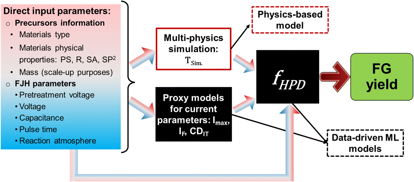 | ||
| Fig. 2 Schematic and data flow of the proposed SML framework, where the temperature simulated by the multi-physics simulation, predicted current parameters, precursor information, and direct FJH parameters are used as the input of the final ML model. | ||
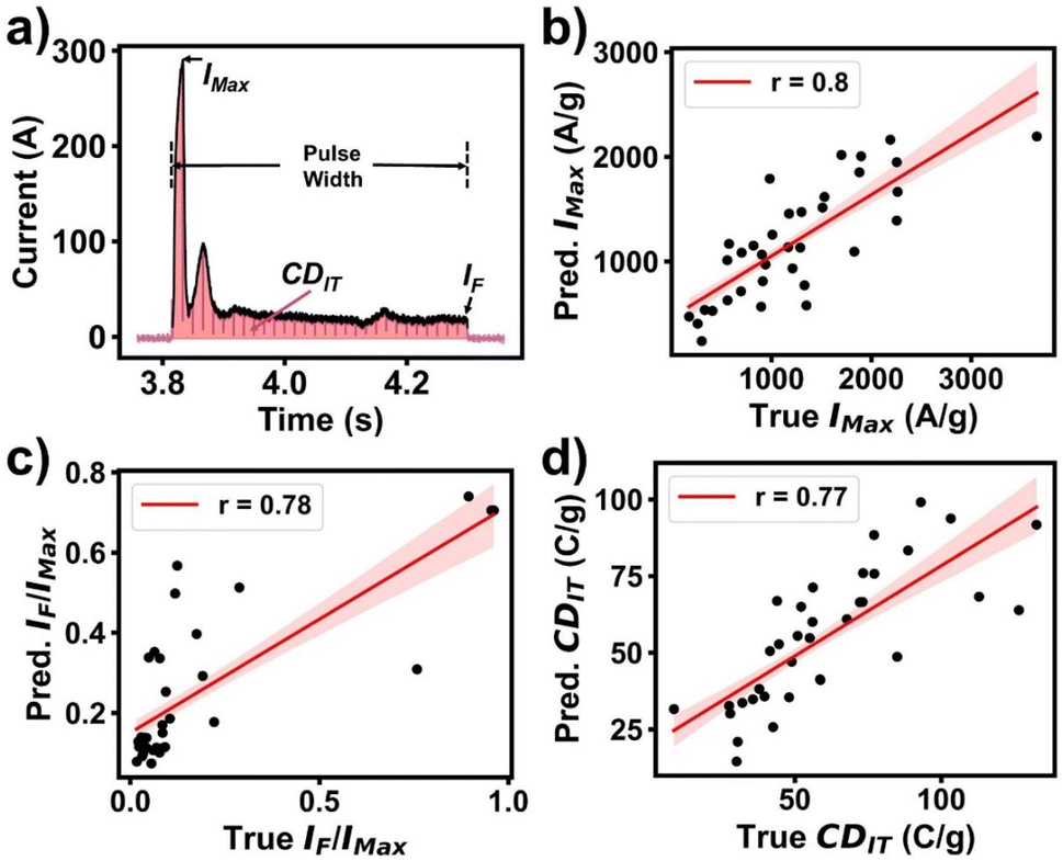 | ||
| Fig. 3 (a) A represented current–time plot and the current parameters derived from it. Distributions of predicted and true (b) IMax; (c) IF/IMax; and (d) CDIT values. Their corresponding Pearson's r values are shown in the figures. | ||
To train the proxy models that predict these three current parameters, the direct reaction parameters, including the properties of starting materials and FJH parameters, serve as the inputs of the models which were trained by a five-fold cross-validation approach. To test the models, 20% of the total samples were used as the never-seen samples. The optimized hyperparameters for these three proxy XGBoost models are listed in Table S2.† It is worth mentioning that the inputs to the proxy models can be hypothesized for predicting reaction outcome of a new experiment without performing it. As a result, the trained models can be used to predict the three current parameters for a new reaction. Fig. 3b–d shows comparison of the predicted three current parameters from the proxy models versus their true values, from which their Pearson's r values can be calculated to evaluate performance of the proxy models. Pearson's r values of 0.80, 0.78, and 0.77 were obtained for IMax, IF/IMax, and CDIT, respectively. The high correlations between the predicted and the true values show that the proxy models can predict the output IMax, IF/IMax, and CDIT from the direct parameters so that no prior-measurement on the current–time curves for a hypothesized FJH experiment would be needed.
In our recent work,15 we conducted an exploratory analysis to examine the influence of various input features on the prediction of FG yield. Through the importance analysis, we determined that the normalized maximum current, the ratio of final to maximum current, and the charge density exhibited were most important. Additionally, we experimented additional features obtained from current–time (I–T) curves, such as the mean current in the I–T curve, the number of local maxima/minima in the I–T curve, and the current-derived properties before normalization. However, these attempted features did not enhance the prediction accuracy and had marginal importance (close to 0) in predicting the FG yield.
In future, it is possible to apply multi-scale simulation techniques such as the one introduced by Talebi et al.35 We hypothesize that collection of the experimental temperature during the reaction for validation, these techniques would render better understanding on the FJH process.
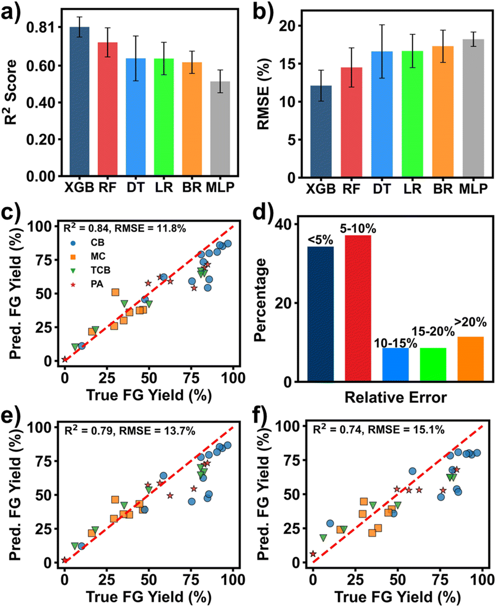 | ||
| Fig. 4 Performance of the ML models in predicting the FG yield. (a) R2 scores and (b) RMSE of the predicted FG yield by the six ML models when using five different train-test splitting ways. The error bars represent the standard deviations from these five testing ways. (c) Plot of predicted FG yields by the XGBoost model vs. their true values from different starting materials. (d) Relative error distribution of the predicted FG yields shown in (c). Plot of the predicted FG yields by the XGBoost model vs. their true values after excluding (e) TSim. and (f) both TSim. and predicted current parameters from the direct input parameters. | ||
To test the significance of including the physics-informed features as the input to the model, we trained a separate XGBoost model without using them as the input. As shown in Fig. 4e, if the TSim. is excluded, the R2 score is reduced to 0.79 and RMSE is increased to 13.7% for the same testing dataset. If both the simulated temperature and the predicted current parameters are excluded, the R2 score is greatly decreased to 0.74 and RMSE is increased to 15.1% (Fig. 4f). This results because the current parameters may reflect the change of the starting materials' resistance and the contact resistance between the starting materials and the electrode over the pulse time. The temperature is a key parameter that determines the reaction outcome. Consequently, these physics-informed descriptors can offer complementary information to the model with increased the prediction accuracy.
2.3 Model interpretation
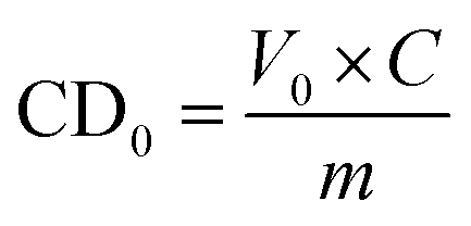
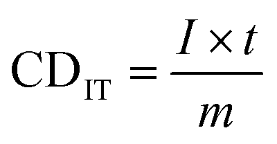
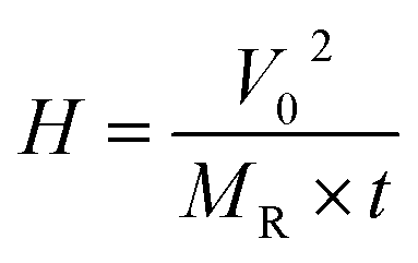
Ranking importance of the input features to the well-trained model in predicting the FG yield would offer additional information about the reaction. The selected features included the CD0, MPS, MR, Msp2, predicted IMax, predicted IF/IMax, predicted CDIT, TSim., t, VPre, Atm, and H. A Pearson's correlation map between these quantitative features is shown in Fig. 5a. Low Pearson's r values between any two features indicate that they are quite independent features for the model to afford accurate prediction. For instance, the correlation of the chosen physical properties of the starting materials is low, indicating that they offer complementary information of the materials properties when serving as the input features. In contrast, the surface area has a high Pearson's r value of 0.9 with the particle size, thus we excluded it from the final input features. Fig. 5b shows the ranking of the features. CD0 and TSim. were ranked the top 2 important features in determining the FG yield, which explains why they play a critical role in the model accuracy (Fig. 4). Other features such as the predicted current parameters also have a significant importance in the final prediction. In previous works,15,36,37 voltage and CD0 were reported to have effects on the transformation rate. Fig. 5c shows that the FJH reactions with low CD0 values have a lower FG yield. In contrast, the ones leading to a high FG yield have high CD0 values. This observation agrees well the results shown in these works. In addition, it is found that there is a CD0 threshold value of 100 (C g−1) for achieving an FG yield of >50%. This observation agrees well with other FFE processes. For instance, laser-induced synthesis of graphene from polymers was only initiated when a laser flux reaches a threshold value.38Fig. 5d shows the importance of TSim. in predicting the FG yield. It shows that when TSim. exceeds a threshold value as indicated in green yellow, and red colors, the FG yield is significantly higher than those with low TSim.. A decision tree extracted from the XGBoost model supports the hypothesis that high TSim. and CD0 are critical in model accuracy for predicting the FG yield (Fig. S6†). Fig. S7† compares CD0 with C, V0, and m in correlating with the FG yield. It shows that correlation of FG yield with CD0 is higher than that with C, V0, and m, which validates the importance of CD0 in the accurate prediction of the FG yield.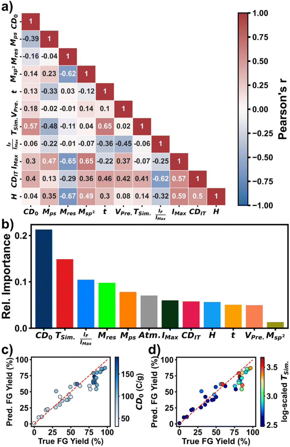 | ||
| Fig. 5 Analysis of the input features to the final XGBoost model. (a) Quantitative correlation map of the input features. (b) Feature importance of the input features. Predicted FG yields versus the true values when correlated with (c) CD0 and (d) TSim.. In (d) TSim. is in a log scale. | ||
3 Conclusion
This study demonstrates an SML framework that bridges a gap between the input processing parameters with the predicted FG yield. Herein, a systematic method of using proxy ML models and multi-physics simulation for extracting physics-informed descriptors, including current-derived properties and simulated temperature, has been developed. These additional input features prove to play a critical role in improving the prediction accuracy of the final ML model. Feature importance analysis further validates this conclusion. Besides the TSim. and CD0, the selected physical properties of the starting materials are also important features. Explainability of the model by the quantitative analysis offers a glimpse on the reaction mechanism about the FJH. In summary, development of this SML framework offers a methodology of predicting the outcome of new experiments, thus saving the cost and time because of performing unnecessary experiments, which would speed up the FG synthesis. Finally, the methodology can be readily applied to other material systems processed by other processing methods.4 Methods and experimental section
4.1 Materials
Four carbon feedstocks were used as the starting materials. They are carbon black (Cabot BP2000), metallurgical coke (SunCoke Energy Inc., 70–100 mesh size, 150–210 μm grain size), pyrolysis ash (Shangqiu Zhongming EcoFriendly Equipment Co.), and pyrolyzed rubber tire-derived carbon black (Ergon Asphalt and Emulsion Co.). We ground the materials using a mortar and pestle before and after FJH.4.2 FJH process
A custom FJH apparatus was used for all the 173 experiments. Precursor powders with a mass between 100 and 400 mg were sandwiched between two graphite electrodes and compressed inside a quartz tube with an inner diameter of 8 mm. Then, a series circuit with eight 6 mF capacitors (Mouser #80-PEH200YX460BQU2), two 5.6 mF capacitors (80-ALS70A562QH500), and nine 18 mF capacitors (Mouser #80-ALS70A183QS400) were used. Arrangement of capacitors was set to reach the peak capacitance values employed in each flash reaction. To charge the capacitors, the voltage was supplied by a DC source consisting of an AC wall outlet fed through an AC–DC converter. FJH reactions were performed inside a desiccator filled with argon, air, or light vacuum (10 mm Hg) that was used as a categorical descriptor for atmosphere type (Atm) among direct input features. After applying the initial voltage, the final voltage was recorded after each reaction. A voltage drop was then calculated by subtracting the final voltage from the initial one. Resistance of the samples were measured before and after each reaction to monitor electrical contact between the electrodes and the samples. Pulse time was modulated by insulated gate bipolar transistors (IGBTs) using programmable millisecond-level delay time. It was connected to a Hall effect sensor through an inductor and controlled via custom LabVIEW scripts. The Hall effect sensor was employed to collect current–time curves. A custom-written Python script was applied on the current–time curves to extract current parameters for the proxy model training.4.3 Material characterization and analysis
Wide-area Raman spectral mapping was selected as the primary method for characterizing the FG property. To mitigate potential biases caused by spatial variations, mapping was conducted on a 1 mm2 region to obtain 64 spectra per mapping. The spectra were acquired using a Renishaw inVia Raman microscope equipped with a 50× lens and a 5 mW 532 nm Nd:YAG laser for excitation. Laser focus was maintained across the area using Renishaw Wire 5.5 LiveTrack software. The resulting spectra were analyzed using the written Python scripts. Before analysis, each spectrum underwent baseline correction using a RamPy polynomial fit and then was smoothened via a Savitzky–Golay filter. A FJ product was categorized as “graphene” was based on the following characteristics of its spectrum: I2D/IG > 0.3, 15 cm−1 < FWHM2D < 70 cm−1, and a signal-to-noise ratio (SNR2D) of > 8. Others were categorized as “amorphous carbon”. Spectra lacking a sufficiently strong G band (SNRG < 8) were excluded from the analysis as they indicated poor laser beam focusing. The FG yield was calculated for each sample by dividing the total number of Raman spectra that were categorized for graphene by the total number of Raman spectra obtained from that sample. This afforded an approximate numerical measure of the sample's bulk crystallinity.4.4 Data inclusion
At the spectra-level, we included all spectra identified as having a G peak with an SNR of >8 (in the range of 1500–1700 cm−1). Spectra not containing a G peak were attributed to poor laser focusing and excluded.4.5 Training of machine learning models
Six different ML models (LR, MLP-R, BR, DT-R, RF-R, and XGB-R) were trained to predict FG yield. The Scikit-Learn package from Python was used for constructing all the models. We kept 20% of the dataset unseen for testing. Cross-validation was applied to optimize the hyperparameters. To test the accuracy of the model for different testing samples, we tried 5 different train/test splits. The results were reported as metrics' mean ± standard deviation.4.6 Feature engineering
Twelve selected features (as tabulated in Table S4†) included the charge density (CD0) released from the capacitors, starting materials' type (M), particle size (MPS), resistance (MR), surface area (MSA), and percent of sp2 content (Msp2), predicted normalized maximum current (IMax), predicted ratios of final current to the maximum current (IF/IMax), predicted charge density that is defined as area under the current–time curve normalized by mass (CDIT), simulated temperature (TSim.), pulse time (t), pre-treatment voltage (VPre), atmosphere type (Atm), and nominal heat (H) were used as the input features to the final ML models.CD0, CDIT, and H are defined in eqn (1)–(3), respectively.
 | (1) |
 | (2) |
 | (3) |
4.7 Evaluation metrics
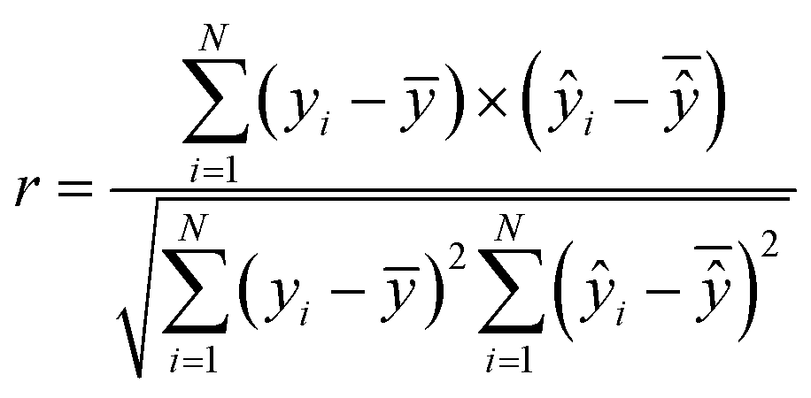
The coefficient of determination (R2) is used to evaluate the prediction accuracy of a model as shown in eqn (4). The Pearson correlation coefficient (r) defined in eqn (5), on the other hand, measures how the predicted values catch the trend compared to the true values.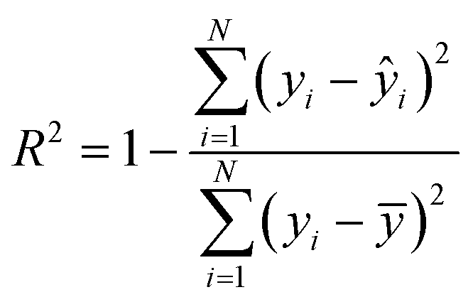 | (4) |
 | (5) |
 is the average of all predicted ŷ.
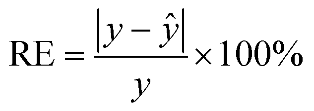
Other evaluation metrics including residuals (R), relative error (RE) and root mean squared error (RMSE) are defined in eqn (6)–(8), respectively.
| R = ŷ − y | (6) |
 | (7) |
 | (8) |
4.8 FEA simulation on temperature
The electrical–thermal multi-physics package in COMSOL Multiphysics version 6.0 licensed under University of Missouri was applied to simulate the temperature evolving over the pulse duration of each reaction. In the simulation, we added three physics interfaces nodes—electric currents, heat transfer in solids, and the multiphysics node. The starting materials mass and particle sizes as well as pulse time, voltage, and capacitance of each reaction were used as the input to the simulation. Also, we considered 140, 130, 120, and 113 (S m−1) for the electrical conductivity and 0.4, 1.2, 2.2, and 2.7 (W m−1 K−1) for the thermal conductivity of the starting materials CB, PA, MC, and TCB, respectively. The applied electrical and thermal conductivity values are in the range of reported experimental values.39–41 To set up the electrical boundary conditions, one side of the simulated cylinder was grounded (0 V) and the other side was applied with the input voltage values shown in the dataset. To set up the heat boundary conditions, we used the room temperature as the initial temperature of the system and applied convective heat flux around the cylinder surfaces. After finding the location with the maximum temperature in each reaction, we used the final simulated temperature (end of each pulse time) of the location as the input to the SML as TSim..Data availability
Data and processing scripts for this paper, including the collected experiments are available at GitHub repository at https://github.com/linresearchgroup/SciML_FJH.Author contributions
J. L. conceived the idea. K. S. designed the framework, constructed the ML models, performed the temperature simulation, and analyzed the data. K. S. wrote the first manuscript which was thoroughly revised by J. L. R. B. assisted K. S. in model development and manuscript writing. J. L. B. provided discussion on the results. L. E. and K. M. W. performed experiments for data collection. J. M. T. supervised L. E., J. L. B., and K. M. W., in the experimental design, data collection as well as revising the manuscript. All authors discussed and commented on the manuscript.Conflicts of interest
Universal Matter Inc. has licensed the FG process from Rice University. J. M. T. is a stockholder in that company, but not an officer, director, or employee. Conflicts of interest are managed through regular disclosure to and compliance with the Rice University Office of Sponsored Programs and Research Compliance.Acknowledgements
J. L. and J. M. T. thank U.S. Army Corps of Engineers, ERDC (grant number: W912HZ-21-2-0050) for the financial support. This work was also partially funded by National Science Foundation (award numbers: 1825352 and 2154428), and the Air Force Office of Scientific Research (FA9550-22-1-0526).References
- Z. Sun, S. Fang and Y. H. Hu, 3D Graphene Materials: From Understanding to Design and Synthesis Control, Chem. Rev., 2020, 120, 10336–10453 CrossRef CAS PubMed.
- K. M. Wyss, D. X. Luong and J. M. Tour, Large-Scale Syntheses of 2D Materials: Flash Joule Heating and Other Methods, Adv. Mater., 2022, 34, 2106970 CrossRef CAS PubMed.
- D. X. Luong, K. V. Bets, W. A. Algozeeb, M. G. Stanford, C. Kittrell, W. Chen, R. V. Salvatierra, M. Ren, E. A. McHugh, P. A. Advincula, Z. Wang, M. Bhatt, H. Guo, V. Mancevski, R. Shahsavari, B. I. Yakobson and J. M. Tour, Gram-scale bottom-up flash graphene synthesis, Nature, 2020, 577, 647–651 CrossRef CAS PubMed.
- K. M. Wyss, J. L. Beckham, W. Chen, D. X. Luong, P. Hundi, S. Raghuraman, R. Shahsavari and J. M. Tour, Converting plastic waste pyrolysis ash into flash graphene, Carbon, 2021, 174, 430–438 CrossRef CAS.
- P. A. Advincula, V. Granja, K. M. Wyss, W. A. Algozeeb, W. Chen, J. L. Beckham, D. X. Luong, C. F. Higgs and J. M. Tour, Waste plastic- and coke-derived flash graphene as lubricant additives, Carbon, 2023, 203, 876–885 CrossRef CAS.
- Y. Wu, P. A. Advincula, O. Giraldo-Londoño, Y. Yu, Y. Xie, Z. Chen, G. Huang, J. M. Tour and J. Lin, Sustainable 3D Printing of Recyclable Biocomposite Empowered by Flash Graphene, ACS Nano, 2022, 16, 17326–17335 CrossRef CAS PubMed.
- R. Raj, Joule heating during flash-sintering, J. Eur. Ceram. Soc., 2012, 32, 2293–2301 CrossRef CAS.
- D. Dai, Q. Liu, R. Hu, X. Wei, G. Ding, B. Xu, T. Xu, J. Zhang, Y. Xu and H. Zhang, Method construction of structure-property relationships from data by machine learning assisted mining for materials design applications, Mater. Des., 2020, 196, 109194 CrossRef CAS.
- J. Yu, X. Yong, Z. Tang, B. Yang and S. Lu, Theoretical Understanding of Structure–Property Relationships in Luminescence of Carbon Dots, J. Phys. Chem. Lett., 2021, 12, 7671–7687 CrossRef CAS PubMed.
- K. Sattari, Y. Xie and J. Lin, Data-driven algorithms for inverse design of polymers, Soft Matter, 2021, 17, 7607–7622 RSC.
- Y. Xie, K. Sattari, C. Zhang and J. Lin, Toward autonomous laboratories: Convergence of artificial intelligence and experimental automation, Prog. Mater. Sci., 2023, 132, 101043 CrossRef.
- P. Raccuglia, K. C. Elbert, P. D. F. Adler, C. Falk, M. B. Wenny, A. Mollo, M. Zeller, S. A. Friedler, J. Schrier and A. J. Norquist, Machine-learning-assisted materials discovery using failed experiments, Nature, 2016, 533, 73–76 CrossRef CAS PubMed.
- Y. Xie, C. Zhang, X. Hu, C. Zhang, S. P. Kelley, J. L. Atwood and J. Lin, Machine Learning Assisted Synthesis of Metal–Organic Nanocapsules, J. Am. Chem. Soc., 2020, 142, 1475–1481 CrossRef CAS PubMed.
- C. Wen, C. Wang, Y. Zhang, S. Antonov, D. Xue, T. Lookman and Y. Su, Modeling solid solution strengthening in high entropy alloys using machine learning, Acta Mater., 2021, 212, 116917 CrossRef CAS.
- J. L. Beckham, K. M. Wyss, Y. Xie, E. A. McHugh, J. T. Li, P. A. Advincula, W. Chen, J. Lin and J. M. Tour, Machine Learning Guided Synthesis of Flash Graphene, Adv. Mater., 2022, 34, 2106506 CrossRef CAS PubMed.
- J. Hoffmann, Y. Bar-Sinai, L. M. Lee, J. Andrejevic, S. Mishra, S. M. Rubinstein and C. H. Rycroft, Machine learning in a data-limited regime: Augmenting experiments with synthetic data uncovers order in crumpled sheets, Sci. Adv., 2019, 5, eaau6792 CrossRef PubMed.
- G. E. Karniadakis, I. G. Kevrekidis, L. Lu, P. Perdikaris, S. Wang and L. Yang, Physics-informed machine learning, Nat. Rev. Phys., 2021, 3, 422–440 CrossRef.
- B. Kapusuzoglu and S. Mahadevan, Physics-Informed and Hybrid Machine Learning in Additive Manufacturing: Application to Fused Filament Fabrication, JOM, 2020, 72, 4695–4705 CrossRef.
- J. Willard, X. Jia, S. Xu, M. Steinbach and V. Kumar, Integrating scientific knowledge with machine learning for engineering and environmental systems, ACM Comput. Surv., 2022, 55, 1–37 CrossRef.
- M. Arias Chao, C. Kulkarni, K. Goebel and O. Fink, Fusing physics-based and deep learning models for prognostics, Reliab. Eng. Syst. Saf., 2022, 217, 107961 CrossRef.
- A. Daw, A. Karpatne, W. Watkins, J. Read and V. Kumar, arXiv, 2021, preprint, arXiv:1710.11431v3, DOI:10.48550/arXiv.1710.11431.
- M. Raissi, P. Perdikaris and G. E. Karniadakis, Physics-informed neural networks: A deep learning framework for solving forward and inverse problems involving nonlinear partial differential equations, J. Comput. Phys., 2019, 378, 686–707 CrossRef.
- C. Anitescu, E. Atroshchenko, N. Alajlan and T. Rabczuk, Artificial Neural Network Methods for the Solution of Second Order Boundary Value Problems, Comput. Mater. Continua, 2019, 59, 345–359 Search PubMed.
- E. Samaniego, C. Anitescu, S. Goswami, V. M. Nguyen-Thanh, H. Guo, K. Hamdia, X. Zhuang and T. Rabczuk, An energy approach to the solution of partial differential equations in computational mechanics via machine learning: Concepts, implementation and applications, Comput. Methods Appl. Mech. Eng., 2020, 362, 112790 CrossRef.
- Z. Ren, L. Gao, S. J. Clark, K. Fezzaa, P. Shevchenko, A. Choi, W. Everhart, A. D. Rollett, L. Chen and T. Sun, Machine learning–aided real-time detection of keyhole pore generation in laser powder bed fusion, Science, 2023, 379, 89–94 CrossRef CAS PubMed.
- S. Sun, A. Tiihonen, F. Oviedo, Z. Liu, J. Thapa, Y. Zhao, N. T. P. Hartono, A. Goyal, T. Heumueller, C. Batali, A. Encinas, J. J. Yoo, R. Li, Z. Ren, I. M. Peters, C. J. Brabec, M. G. Bawendi, V. Stevanovic, J. Fisher and T. Buonassisi, A data fusion approach to optimize compositional stability of halide perovskites, Matter, 2021, 4, 1305–1322 CrossRef CAS.
- X. Huang, D. Lv, C. Zhang and X. Yao, Machine-learning reveals the virtual screening strategies of solid hydrogen-bonded oligomeric assemblies for thermo-responsive applications, Chem. Eng. J., 2023, 456, 141073 CrossRef CAS.
- B. Deng, D. X. Luong, Z. Wang, C. Kittrell, E. A. McHugh and J. M. Tour, Urban mining by flash Joule heating, Nat. Commun., 2021, 12, 5794 CrossRef CAS PubMed.
- B. Deng, P. A. Advincula, D. X. Luong, J. Zhou, B. Zhang, Z. Wang, E. A. McHugh, J. Chen, R. A. Carter, C. Kittrell, J. Lou, Y. Zhao, B. I. Yakobson, Y. Zhao and J. M. Tour, High-surface-area corundum nanoparticles by resistive hotspot-induced phase transformation, Nat. Commun., 2022, 13, 5027 CrossRef CAS PubMed.
- B. Deng, Z. Wang, W. Chen, J. T. Li, D. X. Luong, R. A. Carter, G. Gao, B. I. Yakobson, Y. Zhao and J. M. Tour, Phase controlled synthesis of transition metal carbide nanocrystals by ultrafast flash Joule heating, Nat. Commun., 2022, 13, 262 CrossRef CAS PubMed.
- A. C. Ferrari, Raman spectroscopy of graphene and graphite: Disorder, electron–phonon coupling, doping and nonadiabatic effects, Solid State Commun., 2007, 143, 47–57 CrossRef CAS.
- A. C. Ferrari and D. M. Basko, Raman spectroscopy as a versatile tool for studying the properties of graphene, Nat. Nanotechnol., 2013, 8, 235–246 CrossRef CAS PubMed.
- J. A. Garlow, L. K. Barrett, L. Wu, K. Kisslinger, Y. Zhu and J. F. Pulecio, Large-Area Growth of Turbostratic Graphene on Ni(111) via Physical Vapor Deposition, Sci. Rep., 2016, 6, 19804 CrossRef CAS PubMed.
- L. Van der Maaten and G. Hinton, Visualizing data using t-SNE, J. Mach. Learn. Res., 2008, 9, 2579–2605 Search PubMed.
- H. Talebi, M. Silani, S. P. A. Bordas, P. Kerfriden and T. Rabczuk, A computational library for multiscale modeling of material failure, Comput. Mech., 2014, 53, 1047–1071 CrossRef.
- K. S. Ravi Chandran, Transient Joule heating of graphene, nanowires and filaments: Analytical model for current-induced temperature evolution including substrate and end effects, Int. J. Heat Mass Transfer, 2015, 88, 14–19 CrossRef CAS.
- J. Y. Huang, S. Chen, Z. F. Ren, G. Chen and M. S. Dresselhaus, Real-Time Observation of Tubule Formation from Amorphous Carbon Nanowires under High-Bias Joule Heating, Nano Lett., 2006, 6, 1699–1705 CrossRef CAS PubMed.
- J. Lin, Z. Peng, Y. Liu, F. Ruiz-Zepeda, R. Ye, E. L. G. Samuel, M. J. Yacaman, B. I. Yakobson and J. M. Tour, Laser-induced porous graphene films from commercial polymers, Nat. Commun., 2014, 5, 5714 CrossRef CAS PubMed.
- S. Khodabakhshi, P. F. Fulvio and E. Andreoli, Carbon black reborn: Structure and chemistry for renewable energy harnessing, Carbon, 2020, 162, 604–649 CrossRef CAS.
- D. Pantea, H. Darmstadt, S. Kaliaguine, L. Sümmchen and C. Roy, Electrical conductivity of thermal carbon blacks: Influence of surface chemistry, Carbon, 2001, 39, 1147–1158 CrossRef CAS.
- D. Han, Z. Meng, D. Wu, C. Zhang and H. Zhu, Thermal properties of carbon black aqueous nanofluids for solar absorption, Nanoscale Res. Lett., 2011, 6, 457 CrossRef PubMed.
Footnote |
| † Electronic supplementary information (ESI) available: Features distribution, simulated temperature of reactions inside the quartz tube, ML models' hyperparameters, starting materials' physical properties (PDF). See DOI: https://doi.org/10.1039/d3dd00055a |
| This journal is © The Royal Society of Chemistry 2023 |