Model-based evaluation and data requirements for parallel kinetic experimentation and data-driven reaction identification and optimization

Abstract

Recently there has been growing interest in implementing the high-throughput approach to access the dynamics of chemical processes across different fields. With an ever-increasing amount of data provided by high-throughput experimentation, the development of fully-integrated workflows becomes crucial. These workflows should combine novel experimental tools and interpretation methods to convert the data into valuable information. To design feasible data-driven workflows, it is necessary to estimate the value of information and balance it with the number of experiments and resources required. Basing this kind of workflow on actual physical models appears to be a more feasible strategy as compared to data-extensive empirical statistical methods. Here we show an algorithm that constructs and evaluates kinetic models of different complexity. The algorithm facilitates the evaluation of the experimental data quality and quantity requirements needed for the reliable discovery of the rates driving the corresponding chemical models. The influence of the quality and quantity of data on the obtained results was indicated by the accuracy of the estimates of the kinetic parameters. We also show that this method can be used to find correct reaction scenarios directly from simulated kinetic data with little to no overfitting. Well-fitting models for theoretical data can then be used as a proxy for optimizing the underlying chemical systems. Taking real physical effects into account, this approach goes beyond: we show that with the kinetic models, one can make a direct, unbiased, quantitative connection between kinetic data and the reaction scenario.

---

Introduction

Human intuition is progressively finding itself challenged by computational techniques in the current digital era. Machine learning is aiding, or even improving decisions made based on human intuition.¹ The performance of machine learning methods directly relates to data and its characteristics. Data-driven guidance is already applied to help chemists, chemical engineers, or automated machines make decisions.^2–7 Furthermore, high-throughput experimentation and automation are rapidly gaining popularity in chemistry, focusing the entire field on the adoption of novel data-driven methodologies and workflows.^8–11

In designing data-centered workflows, it is key to understand the required data quantity and quality. While the Design of Experiments (DoE) approach is widely used for guiding chemical decisions, the models it produces are often purely mathematical or statistical.^12–17 A method accounting for physical and chemical effects would provide richer insights into the investigated problems. Such an approach has been proven beneficial in spectroscopy and catalysis.^18–20

Dynamic chemical processes are typically modeled with a system of ordinary differential equations (ODEs) that describe reaction kinetics. Fitting the experimental data to a model can provide single-metric parameters which can be used for the optimization or to gain mechanistic understanding.^21,22 However, modeling more complex processes using intricate ODE systems without excessive simplifications is less frequently pursued.²³ For instance, in the field of catalysis, kinetic studies often rely on formal phenomenological lump methods.²⁴ Recent reports have highlighted the potential of machine learning for the automatic classification of reaction mechanisms based on kinetic data.²⁵ Yet, these approaches neglect the intricate mechanistic details underlying and defining the efficiency of the catalytic transformations.^26,27

The high complexity and elusiveness of catalytic mechanisms make high-throughput experimentation approaches particularly suitable for their investigation. The large volumes of data from such experiments offer rich opportunities for information extraction methods. Catalytic reactions are typically controlled by complex networks of chemical transformations, which are often complicated by various dynamic processes, such as transport phenome and catalyst deactivation, which can be defined by differentials but do not directly tie into the primary catalytic conversion. This complexity is the primary challenge in catalysis modeling, quickly escalating the number of required parameters and differential equations for its comprehensive description.²⁸ Consequently, empirical fitting of data using knowingly over-simplified or traditional models is a common practice that allows to reduce the dimension and extract empirical parameters, which can be further used to describe or optimize the system. However, such approaches may disregard the intricate relations between various parameters, and the resulting optimization may fall short of a chemically informed optimum.

An ODE model can enhance the optimization, while accounting for limits, equilibria, competing reactions, and many other effects, which are otherwise easily overlooked. An accurate system of ODEs would represent a reaction model, creating a direct link between data and proposed reaction pathways, which could be crucial for extracting valuable insights from chemical kinetic data.

Recently, there has been a growing interest in the application of machine learning and AI methods for the analysis of chemical kinetics. Such approaches can be used to discriminate different kinetic scenarios or even predict reaction mechanism.^29,30 Neural networks, including physics-informed neural networks (PINN's),^31,32 have successfully been used to reconstruct kinetic models from chemical data. However, these methods demand extensive data and vast computational resources to construct and operate the networks. To implement wider the automated kinetic modeling approaches in daily catalysis research practice, it is critically important to reduce the entry bar to the kinetic analysis automation and minimize the associated computational costs. With the creation of larger kinetic datasets becoming increasingly commonplace, there is a pressing need for more user-friendly and easily adjustable software that can run efficiently on standard laptops and lab-PCs.

Herein, we report a Chemfit method (Fig. 1) for the design and evaluation of kinetic experiments based on kinetic models. The presented algorithm can both be used to study complex chemical systems and to evaluate the quality of data across multiple kinetic datasets. It is capable of extracting the rate constants of various chemical phenomena directly from the limited kinetic data. Using synthetic data, we evaluate the effect of model complexity on data quality and quantity requirements. We also investigate the aptitude of Chemfit for aiding in the discovery of correct reaction systems. Besides the base algorithm, a complementary Bayesian optimization algorithm is tested. The power and capabilities of the presented approach are tested and illustrated using a homogeneous catalytic ester hydrogenation reaction as a representative example process.^33,34

Fig. 1 Illustration of the Chemfit workflow. Depicted from left to right: first, fitting current data with current systems; second, estimation of data requirements by using a current model, synthetic data, and rate parameter best guesses; third, finding better systems after real measurement, and finally, results and optimization.

The paper is organized as follows. It starts with a concise description of the methods, followed by the results sections, in which the sub-sections Model construction and Synthetic data generation and fitting summarize the central parameters, model, and data fitting process in the research visually and in detail. Next, the sub-section Data quality evaluation presents the analysis of the influence of many data quality and quantity parameters on the veracity of the rates found by Chemfit. In the subsequent Comparison of correct and incorrect models section the accuracy of the method for finding the correct reaction system directly from the kinetic data is explored. Afterwards, the Optimization section compares the accuracy of finding chemical optima using a Bayesian optimizer alongside the used differential model with the rate estimates found by the Chemfit. The conclusion sections of the manuscript summarize the main aspects and evaluation of the algorithms as well as the key results of the analysis.

Methods

Kinetic data were simulated and fitted in python using the jupyter notebook API. The simulations were made with the initial value problem solver from the SciPy.Integrate package. The simulated data were used to analyze the performance of Chemfit, aiming to reconstruct reaction rates directly from the kinetic data. The fitting was done by using the lmfit package to construct a list of parameters that are varied to find optimal fits. The minimize function was used to minimize the R-squared score produced with the scikit-learn r2_score function by comparing the simulation results to the provided data. For the optimization of the initial conditions, the BayesianOptimization package was used. Progress was tracked with the progressbar2 package. The final results were visualized using matplotlib and pandas. The workflow is openly accessible viahttps://github.com/EPiCs-group/ODE_fitter.

The workflow overview for Chemfit is schematically presented in Fig. 1. First, a set of various kinetic models is constructed manually based on formal kinetics and prior chemical knowledge of the system. The set should include models of different complexity ranging from knowingly over-simplified to more complete ones which include all possible reactions and catalytic intermediates. The models are expressed in strings (e.g. “A + B + cat → C + cat”) which is a conventional form to describe kinetic processes. The program contains functions to convert the conventional string notation into Python-interpretable sets of ODE's.

Alternatively, an additional program ChemKinScreen can be used. We developed ChemKinScreen to use a list of all reaction components to compile different kinetic scenarios. It can aid in the exploration when one is uncertain about the choice of the appropriate reaction system. It takes a more modular approach to construct a reaction system, making it possible to explore many similar systems with different reactions. This could drastically reduce the effort required for the identification of the best set of ODE's to represent kinetic data.

Additionally, both programs include functions for making synthetic datasets containing user-defined noise and variations in data resolution, initial reaction conditions, and the number of measured parameters. Using the programs with synthetic data can help in predicting the data quality and quantity required for desired results with a certain reaction model. These insights can be used either to design the experiment or to check the information value of the existing data set. The models are then used to fit the experimental data and the best model can be used to optimize the reaction parameters.

Results and discussion

Model construction

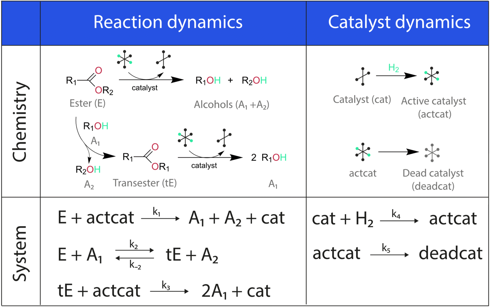
The showcase process chosen to illustrate the extended capabilities of Chemfit is homogeneous catalytic ester hydrogenation reaction. This catalytic process has been extensively studied by our research group in the last decade.^34–37 The extensive literature on catalytic ester hydrogenation has been summarized and critically discussed in several excellent review papers.^{33,34,38–40} This catalytic process is highly complex and besides the main catalytic reaction, often involves catalyst deactivation, product inhibition, formation of various resting states, and in some cases, diffusion limitation.

Fig. 2 depicts the base reaction model of catalytic conversion of an ester substrate to two alcohol products considered in this study. The catalytic reaction is accompanied by such processes as the transesterification that yields a trans-ester by-product/intermediate as well as the catalyst activation (e.g. H₂ activation) and deactivation reactions (e.g. ill-defined degradation paths).²⁷ The activation step is a part of every turnover that yields the reactive hydride catalytic species. The deactivation entails the catalyst species becoming permanently unreactive, resulting in the decreased effective concentration of the catalyst and, accordingly, in the gradual decrease of the reaction rate with time-on-stream. Since the true concentration of the catalyst in the reaction mixture is difficult to access experimentally in situ, our method also aims at providing the means to estimate the dynamics of “hidden” species from measurable ones.

Fig. 2 The reaction scheme for ester hydrogenation used for data synthesis and fitting in this research.

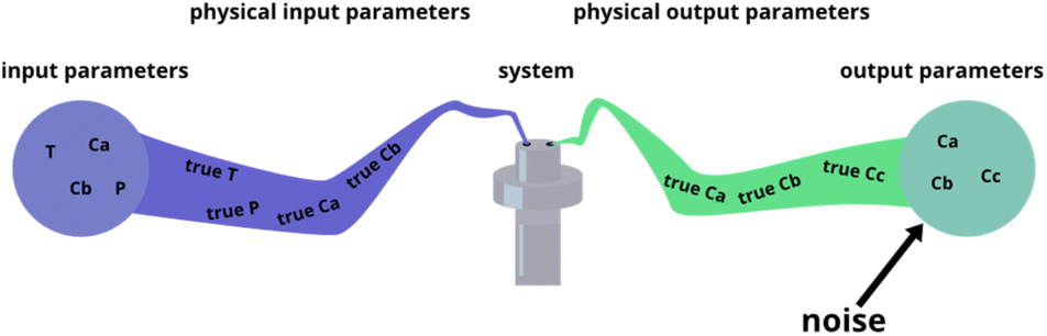
Fig. 3 summarizes two primary parameter classes that determine a chemical process. The first class describes the inherent parameters, including the rate constants (k₁, k₂, etc.), activation energies (E_act1, E_act2, etc.), and pre-exponential factors (A₁, A₂, etc.). The activation energies and pre-exponential factors will henceforth be referred to as the ‘kinetic parameters’ to distinguish them together from the rate constants. The second class describes the variable external initial parameters including temperature (T), hydrogen pressure (P), and the concentrations of the reactants (C_E, C_cat, etc.). Chemfit is developed to recover the inherent parameters from the kinetic data, while the variable parameters add variation to the datasets, thus facilitating the discovery of error.

Fig. 3 Delineation of different system parameters as external (or variable) experimental parameters and inherent (or intrinsic) parameters.

With the chemistry and parameters defined, the ‘base model’ can now be constructed, as expressed in eqn (1)–(7):

The differential model will be referred to as 6k for the six rate constants it uses. This is to distinguish it from simpler sets of ODEs derived from this base model later in the research. Each of the 6 rate constants corresponds to a unique reaction. Thus, k₁ is a forward hydrogenation reaction that converts the initial ester to two alcohols and a dehydrogenated catalyst species (cat); k₂ is the transesterification process, where the ester substrate reacts with the alcohol product to form a trans-ester containing two identical carbon chains at each side of the functional group; k₋₂ is a reverse reaction of k₂; k₃ is a reaction where the catalytic hydrogenation of the trans-ester; k₄ corresponds to a catalyst regeneration reaction, where H₂ is added to reactivate the catalyst and form actcat; and k₅ is a reaction that describes in situ catalyst deactivation/degradation.

A few assumptions were made to construct this ODE system. The first assumption is that hydrogen concentration is constant. This is true when the rate of hydrogen uptake from the gas phase into the reaction mixture is significantly higher than the reaction rate. In other words, we assume that the experiment is performed in a kinetic regime. Diffusion limitation differential equations could also be added if applicable since all phenomena that can be captured in ODEs can be accounted for by Chemfit. Second, in all simulations, the catalyst is initially in its active state. This assumption is made because although in reality there is often an extra pre-catalyst activation step, the rate of this process is typically high compared to the reaction rate. Third, the catalyst deactivation is assumed to only happen to the active complex. The active complex is the most prevalent form, so it was assumed that the majority of deactivation could be captured with a single integral catalyst deactivation process. This is likely a poor reflection of reality but reducing the number of rate constants from 7 to 6 drastically reduces the number of possible parameter combinations. The model can easily be expanded to include all the above-mentioned scenarios depending on extra experimental or computational insights.

Synthetic data generation and fitting

Our approach to evaluating experimental kinetic data involves a fitting procedure where the intrinsic parameters in the set of ODEs are adjusted to minimize the difference between our synthesized dataset and the current estimate. Using an ODE model, it is possible to construct synthetic kinetic datasets with different combinations of initial conditions and intrinsic parameters. This simulation can be insightful on its own, as it allows for visualizing the effect of different parameters on the shape of the resulting kinetic profiles. The simulated datasets can then be used to validate the fitting procedure.

To validate the fitting procedure, we simulate a catalytic ester hydrogenation process. The simulation is carried out at three different temperatures with three different sets of initial conditions. Fig. 4 exhibits the entire initial dataset, along with the successful fits resulting from the accurate rate constant estimates made by Chemfit. The simulated data was then fit using the same ODE system. The multiple datasets obtained for different temperatures and initial concentrations resemble an experiment, in which several kinetic measurements are carried out in parallel. All catalyst-related species are invisible in the fitting procedure, resembling a real-life experiment, in which the determination of all concentrations of kinetically-relevant species in the reaction mixture during the conversion is not possible.

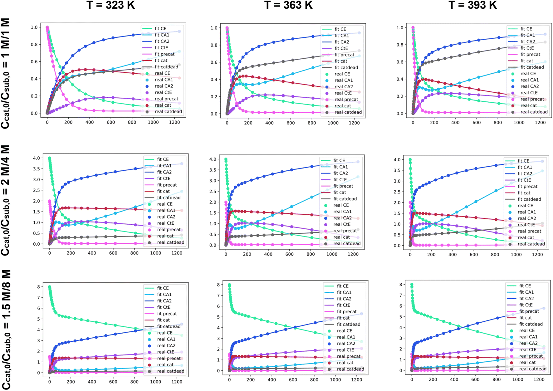Fig. 4 A dataset comprised of 9 computationally simulated kinetics (dots) and generated fits (lines) based on retrieval of fundamental kinetic parameters (E_act, A) for the base model at 3 different temperatures and starting conditions.

To make sure that the rate constants are tuned towards better fits, the difference between the input data and simulated profiles is evaluated with a Levenberg–Marquardt minimizer. To evaluate the goodness of fit, the R² is used as the convergence criterion. After fitting the separate datasets per temperature, the obtained rate constants can be used to estimate kinetic parameters across different temperatures. For the details regarding the procedure used to convert rate constants to kinetic parameters, refer to Section S1 of the ESI.† For more exhibits to illustrate how the Chemfit fits simulated reaction data, and how versatile the method is, refer to Section S2 and Fig. S2–S8 in the ESI.† For validation of the accuracy of the method refer to Section S3 of the ESI.†

Data quality evaluation

The fitting of data to actual reaction progressions allows us not only to characterize Chemfit, but also to estimate what information can accurately be extracted from the data as a function of data quality. Conventionally, reaction system determination is an approximation informed by the species inside a reaction mixture,^41,42 possibly supported by density functional theory (DFT) calculations.⁴³ ODE fitting can serve as a direct connection between data and a reaction scheme, which could majorly reduce speculation. However, the validity of the method should be tested first. The amount of data needed to make good rate constant estimates should be explored theoretically. Besides identifying the data needed to make good estimates for the base model, this is an important quantitative venture into how different data quality metrics affect the reliability of conclusions about details of chemical reaction systems, even if it is through the lens of a fitting algorithm.

To characterize Chemfit's performance and data quality, different factors are considered. We first evaluated the impact of noise on the fitting performance. The noise can be introduced for any parameters of the system, including the initial and dynamic concentration, temperature, pressure, etc., as all these parameters can deviate from the intended set points. Fig. 5 visualizes five instances where noise can occur, and where we added noise to the synthetic datasets. Only output noise, which mimics experimental error in the measurement of dynamic concentrations, is included. In addition, the quality of the prediction as a function of the resolution of the data will be defined. Our analysis also evaluates the effect of reducing the number of measurable species, or combining species into one measurement. Furthermore, it also analyses the effect of the dataset size, due to the number of different temperatures or different initial conditions measured, on the prediction quality.

Fig. 5 Different places where experimental noise can occur, and where it was added for this research.

All results that will be discussed below are an average of 5 simulations run under specified conditions. Finally, measurements of the effect of using correct and incorrect ODE models on the goodness of fit are recorded. After characterizing Chemfit a complementary algorithm that suggests the most efficient conditions based on a user-defined criterion is also evaluated. The following section describes the entire analysis in detail.

Accuracy can be measured with the R-squared of the fits, but that ignores whether the actual rate constants causing the profiles are estimated well. Most importantly, the accuracy of the predicted constants also needs to be evaluated. The accuracy here was measured with the symmetric mean average percentage error (SMAPE, eqn (8)), which is used because the effects of underestimating and overestimating kinetic parameters are deemed equally erroneous. Additional information on the SMAPE is provided in Section S4 and Table S1 of the ESI.†

SMAPE = (abs(k_estimate − k_real)/(k_estimate + k_real))/2 (8)

Effects of noise

Noise is one of the most universally accounted-for factors in experiments. The effects of noise on rate constant estimates can inform researchers of requirements for real-life experimental datasets. The noise was divided into two categories, namely, proportional and structural noise. The proportional noise is made between bounds that are a percentage of the dynamic measured values, whereas the structural noise is made between bounds of a constant number. Both noise components have Gaussian distributions. The obtained kinetic datasets were altered by adding proportional and structural noise, and these were fed to the Chemfit. The proportional noise was varied between 0 and 10% of the measured value, while the structural noise ranged between a flat value of 0–0.5. The scores for the datasets with different amounts of added noise were then evaluated.

Fig. 6 shows a matrix of SMAPE scores for five different levels of the two types of added noise. The proportional noise had a significantly smaller effect on the accuracy of the final estimates than the structural noise. Proportional noise up to 5% is permissible to obtain an accuracy of 95%, yet structural error is almost impermissible for highly accurate conclusions on the parameters that drive a complex system. The results add quantitative numbers to the qualitative claim that noise is detrimental to the data quality, which could help guide researchers on the required data quality for real experiments. For all following simulations, noise parameters of 5% proportional noise and 0.01 structural noise were used. These settings allow the true data to be easily recovered by Chemfit, while not being perfect and resembling real-life experiments.

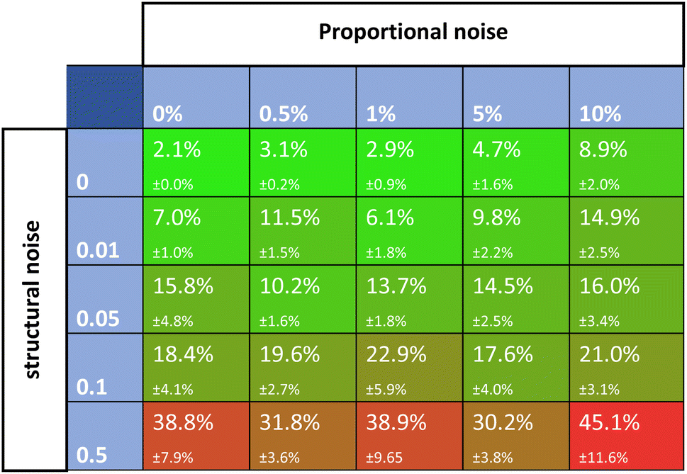Fig. 6 SMAPE scores for different datasets with different levels of proportional and structural noise.

Number of fit metrics

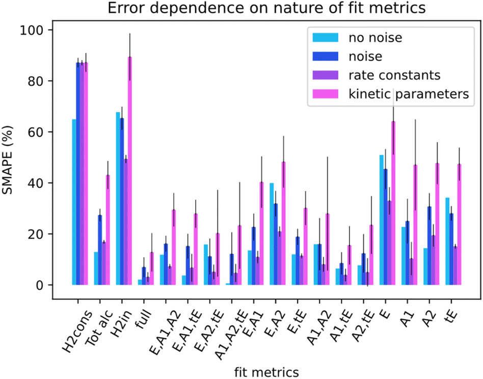
Not all metrics included in a kinetic model can be measured in experiments. For instance, measuring the concentration of catalyst-related species in ester hydrogenation and catalysis with transition metal complexes in general remains challenging and requires the use of advanced spectroscopy methods. Linking the uncoverable complexity with the number of measurable metrics could give insight into measurement requirements. For this section, data from the simulation runs was only partially available to Chemfit. Results were gathered for the full set of all measurable metrics (E, A1, A2, tE), and all combinations of subsets of the base four metrics. In addition, results for select compound metrics, which are a sum or combination of different concentrations, were measured.

Fig. 7 compares the SMAPE scores for noiseless data, noisy data, and separate scores for the rate constants and kinetic parameters for noisy data for multiple sets of metrics. The metrics shown to Chemfit on each test are denoted by the letters on the x-axis, E for ester, A1 and A2 for the alcohols, and tE for the trans ester. ‘Full’ specifies the situation where all 4 measurable metrics are used. To evaluate the performance on metrics that are the result of multiple combined reactions, two types of hydrogen consumption and the total alcohol concentration are also used. It is observed that the nature and number of measurable concentration curves matter. Single metrics were not enough in any case to obtain high accuracy for our complex 6-parameter system. Two metrics performed much better, given that for some combinations the estimates for the rate constants at separate temperatures were reasonably accurate. At three metrics, all rate constant guesses were quite accurate. With the full fitting of all parameters, the rate constants were within 95% accurate. The kinetic parameters never matched the real parameters exactly. However, with the full fitting, the SMAPE was as low as 0.12, which can be seen as an excellent first guess for the kinetic parameters, given the complexity of finding them in general.

Fig. 7 Comparison of SMAPE scores for data without/with noise, and for the rate constant and kinetic parameter estimate error. The x-axis defines which metrics or compound metrics were included in the algorithm runs.

Overall, the data shows that the nature of the metrics plays an important role in the quality of estimates. Our results summarized in Fig. 7 reveal that the datasets containing the substrate concentration E perform noticeably worse than the other datasets centered around the product and intermediates. This can be attributed to a lower sensitivity of this parameter to the changes in other dynamic parameters (concentrations) in the system. Better fitting performance for the datasets which include tE further proves this hypothesis and shows that species that are intrinsically more connected to the secondary processes carry more information.

For the compound metrics, it can be seen that combining metrics is detrimental by virtue of abstracting more specific metrics into single ones. Hydrogen consumption is one of the most commonly used metrics in homogeneous hydrogenation catalysis including the ester hydrogenation reactions. Experimentally, it is relatively easy to monitor this parameter on-line either as a gas flow or pressure drop in the reactor. We consider two alternative situations as shown in Fig. 7, where H2cons represents the hydrogen consumption measured directly from the ODEs, and H2in is the effective hydrogen consumption derived from the combined concentration of all hydrogenated compounds. Tot alc is a metric for when only the total alcohol concentration can be measured. The analysis of the results obtained with these metrics shows that fitting deteriorates when such metrics are combined, instead of being measured separately. The Tot alc metric performed significantly worse than A1 and A2 fit individually and measuring total hydrogen consumption gave the poorest score across the board.

Data resolution

Next, we focused on analyzing the effect of the time resolution of the collected data on the quality of the fits. Well-controlled sampling from running chemical reactors can prove a challenge, thus knowing the value of every extra data point is valuable.⁴⁴ Giving researchers a better view of the required number of data points is beneficial for maximizing results while minimizing experimental effort. For the baseline simulations, the data points were not uniformly distributed over the reaction timespan. The time resolution distributions were modeled in line with the practical kinetic experiments. The time points are denser at the beginning of the time scale where more significant information is contained for a standard batch reactor experiment. The datasets with different time resolutions were provided to Chemfit to observe the effect on the predictions.

Fig. 8 compares the SMAPE scores for the rate constant and subsequent kinetic parameter estimates on datasets, including data with various resolutions. The graph includes estimates on noiseless data and noisy data. Increasing resolution both reduces prediction error, and increases the required amount of algorithm iterations to achieve convergence. Clear asymptotes are observed in the SMAPE scores for both noisy and noiseless data. The 95% certainty threshold for the perfect data could be found using a resolution of only 6 data points. The noise quickly added uncertainty and the 95% certainty threshold increased to approximately 30 points. The comparison of the noisy and noiseless data shows how the error in the prediction of complex chemical models is directly attributable to the quality of the data. Discovering required data quality standards to resolve the intricacies of chemistries is broadly valuable to chemistry. The resolution-dependence of our chosen chemistry and the extent to which noise in kinetic data can be balanced with high resolutions would now be easier to grasp for a researcher.

Fig. 8 SMAPE score as a function of data resolution, generated for data with/without noise.

Number of temperatures, and number of initial conditions

In a typical kinetic experiment, the reaction runs are executed under different initial conditions to better distinguish rate constants and kinetic parameters. These initial conditions can include temperature, pressure, initial concentrations, flows, etc. The variation in initial conditions result in changes of the observed parameters in accordance with the sensitivity of the overall kinetics to these input parameters. We further studied the effect of different initial conditions and a number of varied parameters on the algorithm performance.

The temperature points used for the baseline simulations were 323, 363, and 393 K. Richer datasets are extended with simulations at 423, 293, and 453 K in that order. When the number of temperatures is decreased, the run at 323 K is removed. We further extended the scope with the initial substrate concentration and the initial catalyst concentration. The concentrations will be noted as (substrate concentration in moles, and catalyst concentration in moles) for a more convenient notation. The base values used were (1,1), (4,2), (8,1.5). These were extended with simulations at (5,5), (1,0.2), and (8,8) in respective order as the number of initial conditions increased. When decreased, the initial condition of (8,1.5) and (4,2) are removed in respective order. The catalyst concentration is increased in order because the solver performs better for similar concentrations and low rates. Changing the absolute concentration is irrelevant to the results because the change in catalyst concentration can be compensated by adjusting the affected rate constants. The resulting datasets of varying dimensions were fed to Chemfit, and the effect on the results was documented.

The two charts in Fig. 9 depict Chemfits accuracy on datasets of different dimensions with respect to the number of included temperatures and initial conditions. Expectingly, more data was beneficial to the prediction quality. For the number of initial conditions, all extra data increased estimate accuracy. The return on extra data diminished gradually, but with every addition, the SMAPE was reduced. At two temperatures, the error is extremely high compared to other measurements. If the measurements were gathered using more than two temperature points, the error was very stable. These data imply that in an experimental design, if two temperatures are accounted for, an additional temperature point will provide maximal value. Beyond 3 temperatures, measuring reaction kinetics at a new initial concentration would likely be most valuable. With power for data quality requirement estimation now extensively exhibited, we also looked into Chemfits proficiency as a reaction pathway identification tool.

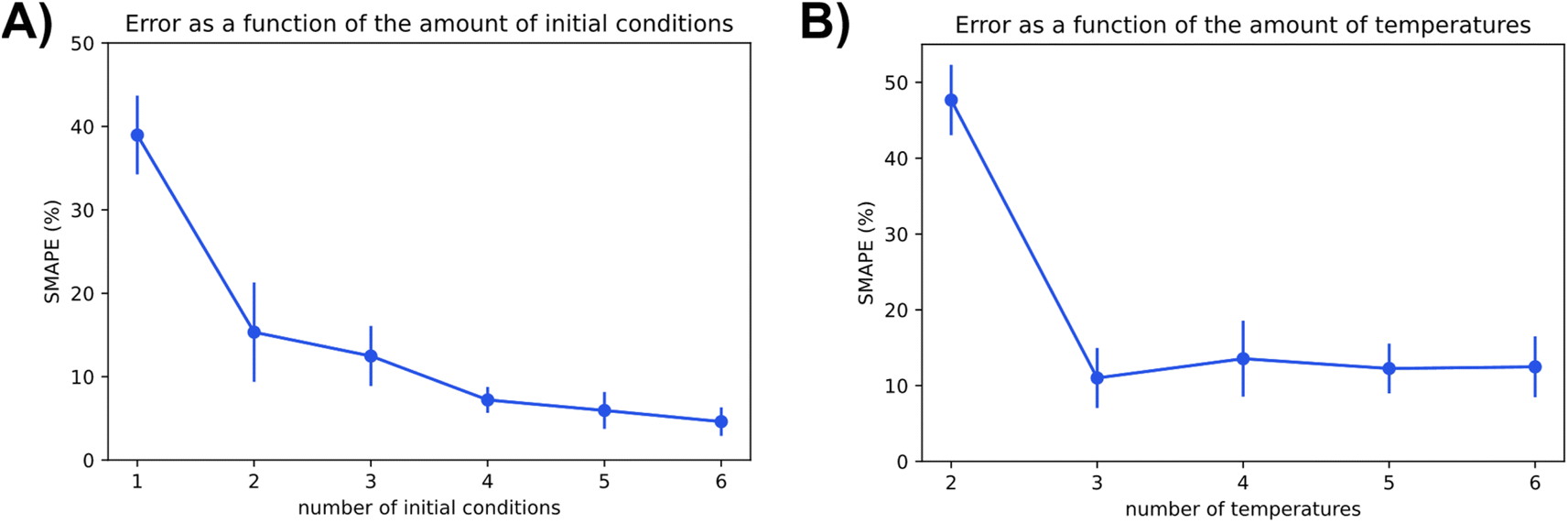Fig. 9 The effect of the conditions parameter space covered in the data on the accuracy of kinetic parameter extraction visualized by SMAPE dependence on the number of different included (A) initial conditions and (B) temperature points.

Comparison of correct and incorrect models

To find accurate underlying chemistries from kinetic data, researchers will need to test multiple different ones. To map the tendencies of ODE fitting, complex data should fit with simple sets of differentials, and simple data should be fit with complex differentials. If models similar to the ones used to generate the data give better scores, it serves as the first proof of the viability of the method as a classification tool. Here the SMAPE is not used since the constants in different models do not correspond to each other. Residuals of the scipy.r2_score for evaluation were used instead. Subsystems were made based on the main model to test whether Chemfit converges to the right solution.

Sub-models

For research into the prediction accuracy with wrong ODEs, simpler models were constructed. Here, different complexities of the base reaction network were removed. The sets of ODEs were named after the number of kinetic constants in the reaction scheme (1k, 2k, 3k, 4k_cat, 4k_tE, 5k, 6k). Fig. 10 illustrates how all subsystems relate to the base model by enclosing the reactions included in each of them, in different colors.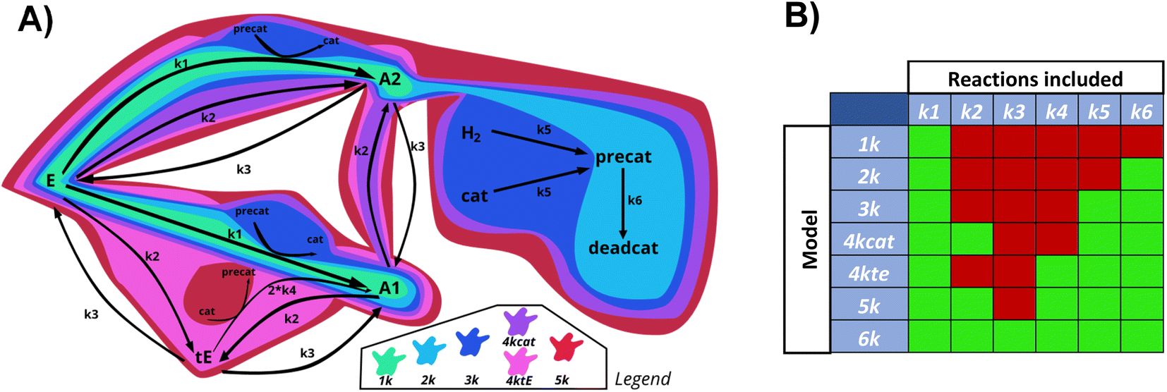

Fig. 10 Schematic overview (A) and table (B) of the reactions included in the main reaction system, and all derived subsystems used for testing Chemfit. Green = 1k, light blue = 2k, dark blue = 3k, purple = 4k_cat, pink = 4k_tE, red = 5k, total = 6k.

The order of incorporating various effects can be based on intuition about which processes are most crucial to the system. As complexity rises, the catalytic cycle is reintegrated first due to its central role. We divided the 4-constant reaction schemes into two, to examine if prioritizing different effects first influences the evaluation. The reverse reaction is added last as the additional trans ester pathway is likely to have a greater impact than the reaction equilibrium. We calculated the errors of fitting for datasets generated with all the models, and then fitted all data with all different models.

Fig. 11 summarizes the residuals for cross-fitting datasets, that are generated using all systems of ODEs. Highlighted in red, are the simulations that fail the rate constant estimation, the subsequent kinetic parameter estimation, or have high residuals. Successful simulations are shown in green. For a lot of fitting methods, overfitting is a big problem. In case of overfitting, complex models would report lower errors than the appropriate models. The obtained scores attained with Chemfit however, point towards the correct model to provide the lowest error, as compared to both the simpler or more complex models; thus, indicating that the data is not being overfit to higher complexity. If the simplest set of differentials is accepted when comparable accuracies occur, all data would be classified correctly. This classification is robust, even if poorer quality data with 10% variable noise and 0.1 proportional noise is evaluated. These results show the potential of this method as a classification tool. With two applications of the method now mapped, we explored the final one, which investigates how an accurate fitting can aid in chemical reaction optimization.

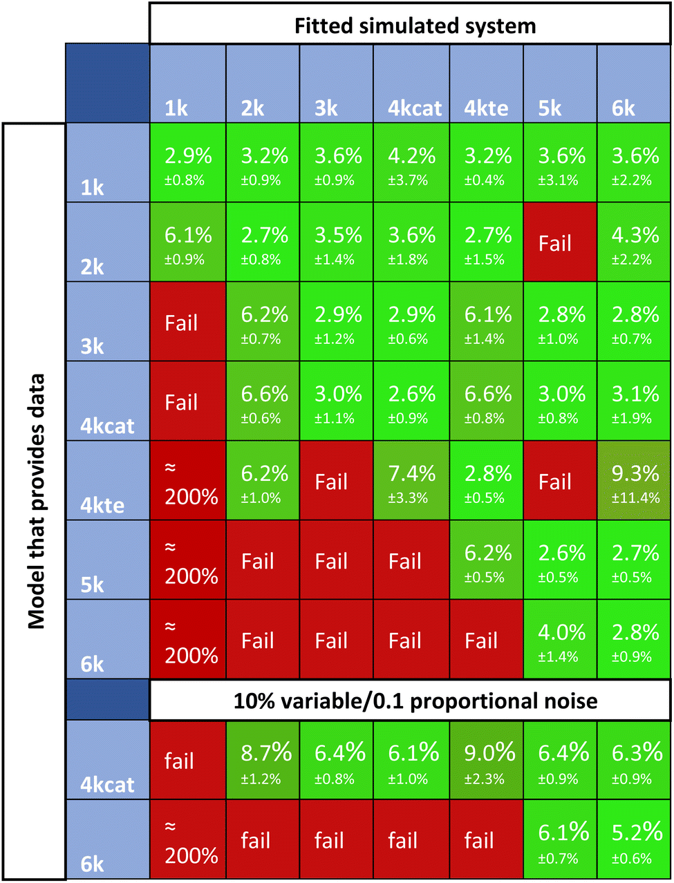Fig. 11 Differences in scores between correctly and incorrectly fit data, the rows indicate the models that provided the data that is fit, and the columns indicate the models used to fit that data. Fail means that Chemfit stopped optimizing an estimation since discrepancies were too high.

Optimization

If representative fits can adequately describe a chemical reaction progression, they can save valuable time as stand-ins for real experiments in reaction optimization. This section is dedicated to exploring whether systems with rate parameter errors can give representative optimization results. 4 parameters were optimized to yield the maximum amount of alcohol per catalyst per substrate (C_A1/(C_cat × C_s)). These were:

• Temperature (T), varied between 293 K and 453 K;

• Pressure (P), varied between 40 and 50 bar;

• The initial concentration of catalyst (C_cat), varied between 0.1 and 2;

• The initial concentration of substrate (C_s), varied between 1 and 10.

The ranges are put into a Bayesian optimizer with a kappa parameter of 1.5, 50 initial random points and 500 selected points. It uses the reaction model either with the true parameters or estimates with a certain error to find the conditions that give an optimal score for the used kinetic parameters.

Table 1 catalogues a comparison of optimizations using a model with the true kinetic parameters to optimizations using sets of differentials with estimated parameters. In the bottom row the yields for the found conditions put into the accurate system are also collected. We observe that the optimizations aiming to uncover a delicate maximum are accurate up to a SMAPE of at least 10%. If parameters are kept within about 10% error, the proposed optimum conditions give yields that are only 1–4% off of the best value compared to the total range of possible scores. This proves this method can be used to find the optima for complex systems with high accuracy despite the presence of reasonable error.

Table 1 Comparison of Bayesian optimization guided optimum initial condition exploration for systems of varying kinetic parameter accuracy

Optimized parameter	Accurate constants	5% SMAPE estimate	10% SMAPE estimate	20% SMAPE estimate	40% SMAPE estimate
T (K)	397	407	388	453	328
P (bar)	50	50	50	50	50
C cat,0 (mol)	0.481	0.507	0.580	0.1	0.163
C s,0 (mol)	1.00	1.00	1.00	1	1
Found conditions yield for accurate parameter model	0.792	0.789	0.791	0.730	0.712

---

Conclusion

Fitting the kinetic data and evaluating the validity of different kinetic models remains challenging in the field of catalysis. Even for a seemingly simple catalytic process, multiple parameters can affect the interpretation of the data. As we show in this work, it is crucial to take these parameters into account and to design the kinetic experiments accordingly. We evaluated the effect of the experimental error, the number of measured metrics, dataset size, and data resolution on the quality of the resulting estimates of kinetic parameters.

Our data show that noise is detrimental to the data quality, especially if it is inherent to a measurement method, and of an order close to the measured values. The structural error should be minimized to be orders of magnitude lower than the measured values to achieve high accuracy. Increasing or separating the number of measurable metrics is nearly always beneficial for data quality. Increasing the number of datasets through the addition of temperature or initial condition points is also always beneficial. Adding datasets at a different temperature is overwhelmingly beneficial if two temperatures are included but adding more barely influences the data quality. Adding datasets at different initial conditions is less significant than adding a third temperature, but every extra initial condition added is valuable regardless of the number of conditions already included. Higher time resolution always increases the quality of the extracted information.

The cross-fitting results showed that the method has little bias towards under-fitting and even over-fitting, which is often seen as a persistent problem with mathematical optimization algorithms. These results show the accuracy of the method for finding reaction systems directly from data. When models that tightly fit the data are found one can assume these models represent the underlying chemistry well. Reaction optimization can be done with such models as stand-ins. We show that expensive experiments can be substituted with well-fitting models, while simulations still yield valuable rich kinetic information, leading to good, chemically informed optimizations. With Chemfit researchers can run tests similar to the ones in this paper, on their chemistries, and discover as well as utilize the connection between their experimental data and theoretical models.

The presented method is a theoretical proof of concept showing that kinetic data quality quantification and linking data directly to reaction systems can be done with ODE-based fitting. The method could be of significant help in proving quantitatively which models are eligible to represent experimental chemistry. In addition, the design of experiments that goes beyond response surfaces based on varied parameters can be done. Optimizations using ODE-based models can take all kinetics in a reaction system into account while retrieving results with simple simulations instead of expensive experiments. Furthermore, the versatility of the method toward different types of kinetic data, differential systems, and inputs could prove useful to the rise of high-throughput experimentation, and data-driven chemical discovery.

In conclusion, Chemfit serves as an encouragement to combine the current power of computer and data science, but eliminate the black box behavior of many algorithms by grounding the approaches in chemically accurate models. When physical effects are present their ability to give context to bare data science should not be disregarded, if not for improved performance, then for understanding of the models. Our method could initially be validated on increasingly complex real data. If the method proves to give accurate insights it could serve as a new standard in utilization of kinetic datasets, and reduce speculation in finding the real chemistry driving them. With the advent of automated chemical machines, Chemfit and optimizations using it might be appropriate fits for autonomous reaction testing, mapping and optimization. Furthermore, this approach can be used to guide the researcher in development of an optimal kinetic experiment.

Data availability

The source code and complete dataset for this paper can be found at https://github.com/EPiCs-group/ODE_fitter.

Author contributions

Nathan Jiscoot: investigation, software, visualization, writing – original draft; Evgeny Uslamin: supervision, methodology, conceptualization, writing – review & editing; Evgeny Pidko: supervision, writing – review & editing, funding acquisition.

Conflicts of interest

There are no conflicts to declare.

Notes and references

1. A. Agrawal, J. Gans and A. Goldfarb, Prediction Machines, Harvard Business Review Press, 2018.
2. J. Timoshenko, D. Lu, Y. Lin and A. I. Frenkel, Supervised Machine-Learning-Based Determination of Three-Dimensional Structure of Metallic Nanoparticles, J. Phys. Chem. Lett., 2017, 8(20), 5091–5098,  DOI:10.1021/acs.jpclett.7b02364.
3. G. A. Landrum, J. E. Penzotti, S. Putta, Y. Xu, Y. Zong, K. Hippalgaonkar, X. Chong, S.-L. Shang and A. M. Krajewski, Machine-Learning Models for Combinatorial Catalyst Discovery, Meas. Sci. Technol., 2005, 16(1), 270–277,  DOI:10.1088/0957-0233/16/1/035.
4. M. Erdem Günay and R. Yıldırım, Recent Advances in Knowledge Discovery for Heterogeneous Catalysis Using Machine Learning, Catal. Rev.: Sci. Eng., 2021, 63(1), 120–164,  DOI:10.1080/01614940.2020.1770402.
5. Y. Shen, J. E. Borowski, M. A. Hardy, R. Sarpong, A. G. Doyle and T. Cernak, Automation and Computer-Assisted Planning for Chemical Synthesis, Nat. Rev. Methods Primers, 2021, 1(1), 23,  DOI:10.1038/s43586-021-00022-5.
6. D. Angelone, A. J. S. S. Hammer, S. Rohrbach, S. Krambeck, J. M. Granda, J. Wolf, S. Zalesskiy, G. Chisholm and L. Cronin, Convergence of Multiple Synthetic Paradigms in a Universally Programmable Chemical Synthesis Machine, Nat. Chem., 2021, 13(1), 63–69,  DOI:10.1038/s41557-020-00596-9.
7. Y. Xu, Y. Zong and K. Hippalgaonkar, Machine Learning-Assisted Cross-Domain Prediction of Ionic Conductivity in Sodium and Lithium-Based Superionic Conductors Using Facile Descriptors, J. Phys. Commun., 2020, 4, 055015,  DOI:10.1088/2399-6528/ab92d8.
8. D. Farrusseng, High-Throughput Heterogeneous Catalysis, Surf. Sci. Rep., 2008, 63(11), 487–513,  DOI:10.1016/j.surfrep.2008.09.001.
9. N. Artrith, K. T. Butler, F. X. Coudert, S. Han, O. Isayev, A. Jain and A. Walsh, Best Practices in Machine Learning for Chemistry, Nat. Chem., 2021, 13(6), 505–508,  DOI:10.1038/s41557-021-00716-z.
10. L. Wilbraham, S. H. M. Mehr and L. Cronin, Digitizing Chemistry Using the Chemical Processing Unit: From Synthesis to Discovery, Acc. Chem. Res., 2021, 54(2), 253–262,  DOI:10.1021/acs.accounts.0c00674.
11. For chemists, the AI revolution has yet to happen, Editorial article, Nature, 2023, 617, 438,  DOI:10.1038/d41586-023-01612-x.
12. R. Leardi, Experimental Design in Chemistry: A Tutorial, Anal. Chim. Acta, 2009, 652(1–2), 161–172,  DOI:10.1016/J.ACA.2009.06.015.
13. P. M. Murray, T. D. Sheppard, F. Bellany, L. Benhamou, D.-K. Bučar and A. B. Tabor, The Application of Design of Experiments (DoE) Reaction Optimisation and Solvent Selection in the Development of New Synthetic Chemistry Organic & Biomolecular Chemistry, Org. Biomol. Chem., 2016, 14(8), 2373–2384,  10.1039/C5OB01892G.
14. R. K. A. van Schendel, W. Yang, E. A. Uslamin and E. A. Pidko, Utilizing Design of Experiments Approach to Assess Kinetic Parameters for a Mn Homogeneous Hydrogenation Catalyst, ChemCatChem, 2021, 13(23), 4886–4896,  DOI:10.1002/cctc.202101140.
15. S. G. Bawa, A. Pankajakshan, C. Waldron, E. Cao, F. Galvanin and A. Gavriilidis, Rapid Screening of Kinetic Models for Methane Total Oxidation Using an Automated Gas Phase Catalytic Microreactor Platform, Chem.: Methods, 2023, 3, e202200049,  DOI:10.1002/cmtd.202200049.
16. C. Waldron, A. Pankajakshan, M. Quaglio, E. Cao, F. Galvanin and A. Gavriilidis, Closed-Loop Model-Based Design of Experiments for Kinetic Model Discrimination and Parameter Estimation: Benzoic Acid Esterification on a Heterogeneous Catalyst, Ind. Eng. Chem. Res., 2019, 58(49), 22165–22177,  DOI:10.1021/acs.iecr.9b04089.
17. G. Franceschini and S. Macchietto, Model-Based Design of Experiments for Parameter Precision: State of the Art, Chem. Eng. Sci., 2008, 63(19), 4846–4872,  DOI:10.1016/J.CES.2007.11.034.
18. J. L. Lansford and D. G. Vlachos, Infrared Spectroscopy Data- and Physics-Driven Machine Learning for Characterizing Surface Microstructure of Complex Materials, Nat. Commun., 2020, 11(1), 1–12,  DOI:10.1038/s41467-020-15340-7.
19. Z. Chen, N. Andrejevic, N. C. Drucker, T. Nguyen, R. P. Xian, T. Smidt, Y. Wang, R. Ernstorfer, D. A. Tennant, M. Chan and M. Li, Machine Learning on Neutron and X-Ray Scattering and Spectroscopies, Chem. Phys. Rev., 2021, 2(3), 031301,  DOI:10.1063/5.0049111.
20. K. Jorner, T. Brinck, P.-O. Norrby and D. Buttar, Machine Learning Meets Mechanistic Modelling for Accurate Prediction of Experimental Activation Energies, Chem. Sci., 2021, 12(3), 1163–1175,  10.1039/D0SC0489H.
21. T. Santra, Fitting Mathematical Models of Biochemical Pathways to Steady State Perturbation Response Data without Simulating Perturbation Experiments, Sci. Rep., 2018, 8(1), 11679,  DOI:10.1038/s41598-018-30118-0.
22. B. Rosenbaum and B. C. Rall, Fitting Functional Responses: Direct Parameter Estimation by Simulating Differential Equations, Methods Ecol. Evol., 2018, 9(10), 2076–2090,  DOI:10.1111/2041-210X.13039.
23. D. G. Blackmond, Reaction Progress Kinetic Analysis: A Powerful Methodology for Mechanistic Studies of Complex Catalytic Reactions, Angew. Chem., Int. Ed., 2005, 44(28), 4302–4320,  DOI:10.1002/anie.200462544.
24. T. Zhang, Y. Zhang, W. E and Y. Ju, DLODE: A Deep Learning-Based ODE Solver for Chemistry Kinetics, AIAA Scitech 2021 Forum, 2021,  DOI:10.2514/6.2021-1139.
25. J. Burés and I. Larrosa, Organic Reaction Mechanism Classification Using Machine Learning, Nature, 2023, 613, 689–695,  DOI:10.1038/s41586-022-05639-4.
26. G. B. Marin, V. V. Galvita and G. S. Yablonsky, Kinetics of Chemical Processes: From Molecular to Industrial Scale, J. Catal., 2021, 404, 745–759,  DOI:10.1016/J.JCAT.2021.09.014.
27. W. Yang, G. A. Filonenko and E. A. Pidko, Performance of Homogeneous Catalysts Viewed in Dynamics, Chem. Commun., 2023, 59(13), 1757–1768,  10.1039/d2cc05625a.
28. Y. Wang, S. Zou and W.-B. Cai, Recent Advances on Electro-Oxidation of Ethanol on Pt- and Pd-Based Catalysts: From Reaction Mechanisms to Catalytic Materials, Catalysts, 2015, 5, 1507–1534,  DOI:10.3390/catal5031507.
29. C. J. Taylor, H. Seki, F. M. Dannheim, M. J. Willis, G. Clemens, B. A. Taylor, T. W. Chamberlain and R. A. Bourne, An Automated Computational Approach to Kinetic Model Discrimination and Parameter Estimation, React. Chem. Eng., 2021, 6(8), 1404–1411,  10.1039/d1re00098e.
30. C. W. Gao, J. W. Allen, W. H. Green and R. H. West, Reaction Mechanism Generator: Automatic Construction of Chemical Kinetic Mechanisms, Comput. Phys. Commun., 2016, 203, 212–225,  DOI:10.1016/J.CPC.2016.02.013.
31. Q. Li, H. Chen, B. C. Koenig and S. Deng, Bayesian Chemical Reaction Neural Network for Autonomous Kinetic Uncertainty Quantification, Phys. Chem. Chem. Phys., 2023, 25, 3707–3717,  10.1039/d2cp05083h.
32. W. Ji, W. Qiu, Z. Shi, S. Pan and S. Deng, Stiff-PINN: Physics-Informed Neural Network for Stiff Chemical Kinetics, CEUR Workshop Proc., 2021, 2964, 1–26.
33. J. R. Cabrero-Antonino, R. Adam, V. Papa and M. Beller, Homogeneous and Heterogeneous Catalytic Reduction of Amides and Related Compounds Using Molecular Hydrogen, Nat. Commun., 2020, 11(1), 1–18,  DOI:10.1038/s41467-020-17588-5.
34. J. Pritchard, G. A. Filonenko, R. Van Putten, E. J. M. Hensen and E. A. Pidko, Heterogeneous and Homogeneous Catalysis for the Hydrogenation of Carboxylic Acid Derivatives: History, Advances and Future Directions, Chem. Soc. Rev., 2015, 44(11), 3808–3833,  10.1039/c5cs00038f.
35. G. A. Filonenko, M. J. B. Aguila, E. N. Schulpen, R. Van Putten, J. Wiecko, C. Müller, L. Lefort, E. J. M. Hensen and E. A. Pidko, Bis-N-Heterocyclic Carbene Aminopincer Ligands Enable High Activity in Ru-Catalyzed Ester Hydrogenation, J. Am. Chem. Soc., 2015, 137(24), 7620–7623,  DOI:10.1021/jacs.5b04237.
36. R. K. A. Van Schendel, W. Yang, E. A. Uslamin and E. A. Pidko, Utilizing Design of Experiments Approach to Assess Kinetic Parameters for a Mn Homogeneous Hydrogenation Catalyst, ChemCatChem, 2021, 13(23), 4886–4896,  DOI:10.1002/cctc.202101140.
37. W. Yang, T. Y. Kalavalapalli, A. M. Krieger, T. A. Khvorost, I. Y. Chernyshov, M. Weber, E. A. Uslamin, E. A. Pidko and G. A. Filonenko, Basic Promotors Impact Thermodynamics and Catalyst Speciation in Homogeneous Carbonyl Hydrogenation, J. Am. Chem. Soc., 2022, 144(18), 8129–8137,  DOI:10.1021/jacs.2c00548.
38. P. A. Dub, Alkali Metal Alkoxides in Noyori-Type Hydrogenations, Eur. J. Inorg. Chem., 2021, 2021(47), 4884–4889,  DOI:10.1002/ejic.202100742.
39. P. A. Dub and T. Ikariya, Catalytic Reductive Transformations of Carboxylic and Carbonic Acid Derivatives Using Molecular Hydrogen, ACS Catal., 2012, 2(8), 1718–1741,  DOI:10.1021/cs300341g.
40. R. Qu, K. Junge and M. Beller, Hydrogenation of Carboxylic Acids, Esters, and Related Compounds over Heterogeneous Catalysts: A Step toward Sustainable and Carbon-Neutral Processes, Chem. Rev., 2023, 123(3), 1103–1165,  DOI:10.1021/acs.chemrev.2c00550.
41. M. Finn, J. A. Ridenour, J. Heltzel, C. Cahill and A. Voutchkova-Kostal, Next-Generation Water-Soluble Homogeneous Catalysts for Conversion of Glycerol to Lactic Acid, Organometallics, 2018, 37(9), 1400–1409,  DOI:10.1021/acs.organomet.8b00081.
42. A. Kulkarni, S. Siahrostami, A. Patel and J. K. Nørskov, Understanding Catalytic Activity Trends in the Oxygen Reduction Reaction, Chem. Rev., 2018, 118(5), 2302–2312,  DOI:10.1021/acs.chemrev.7b00488.
43. M. Garbe, K. Junge and M. Beller, Homogeneous Catalysis by Manganese-Based Pincer Complexes, Eur. J. Org. Chem., 2017, 2017(30), 4344–4362,  DOI:10.1002/ejoc.201700376.
44. I. Tsamardinos, G. S. Fanourgakis, E. Greasidou, E. Klontzas, K. Gkagkas and G. E. Froudakis, An Automated Machine Learning Architecture for the Accelerated Prediction of Metal-Organic Frameworks Performance in Energy and Environmental Applications, Microporous Mesoporous Mater., 2020, 300, 110160,  DOI:10.1016/j.micromeso.2020.110160.

---

Footnotes

† Electronic supplementary information (ESI) available. See DOI: https://doi.org/10.1039/d3dd00016h

‡ Current address: CyberHydra B.V., Delft, The Netherlands.

---