
 Open Access Article
 This Open Access Article is licensed under a Creative Commons Attribution-Non Commercial 3.0 Unported Licence
Designing catalysts with deep generative models and computational data. A case study for Suzuki cross coupling reactions†
Oliver
Schilter
 *ab,
Alain
Vaucher
ab,
Philippe
Schwaller‡
b and
Teodoro
Laino
ab
*ab,
Alain
Vaucher
ab,
Philippe
Schwaller‡
b and
Teodoro
Laino
ab
aIBM Research Europe, Säumerstrasse 4, 8803 Rüschlikon, Switzerland. E-mail: oli@zurich.ibm.com
bNational Center for Competence in Research-Catalysis (NCCR-Catalysis), Switzerland
First published on 17th April 2023
Abstract
The need for more efficient catalytic processes is ever-growing, and so are the costs associated with experimentally searching chemical space to find new promising catalysts. Despite the consolidated use of density functional theory (DFT) and other atomistic models for virtually screening molecules based on their simulated performance, data-driven approaches are rising as indispensable tools for designing and improving catalytic processes. Here, we present a deep learning model capable of generating new catalyst-ligand candidates by self-learning meaningful structural features solely from their language representation and computed binding energies. We train a recurrent neural network-based Variational Autoencoder (VAE) to compress the molecular representation of the catalyst into a lower dimensional latent space, in which a feed-forward neural network predicts the corresponding binding energy to be used as the optimization function. The outcome of the optimization in the latent space is then reconstructed back into the original molecular representation. These trained models achieve state-of-the-art predictive performances in catalysts' binding energy prediction and catalysts' design, with a mean absolute error of 2.42 kcal mol−1 and an ability to generate 84% valid and novel catalysts.
1 Introduction
The need for better and more sustainable catalysts is one of the biggest problems facing the chemical industry. Cross-coupling reactions are a typical example of a chemical reaction scheme used to make C–C bonds.1 They are so widely adopted in industrial applications that a more sustainable, cheaper, and more selective homogeneous catalyst would have a significant socio-economic impact. In particular, the Suzuki–Miyaura cross-coupling reaction has gained popularity due to its mild reaction conditions, high tolerance towards a variety of functional groups and commercial availability and stability of reagents.2 In this reaction scheme, catalysts play a crucial role and the development of new or improved ones is always a topic of greatest interest, which has recently been addressed by favoring data-driven approaches over exhaustive searches.3Some approaches, such as high-throughput screening (HTS), are experimentally driven strategies for catalyst searches. In HTS, a large selection of catalysts, reactants, and solvents are screened in an automated fashion (often carried out on a highly robotized synthesis platform) to find a better-suited catalyst or the best-performing reaction conditions.4,5 Because testing all possible combinations of a relatively small set of reactants, solvents and catalysts leads to an exponential increase in the complexity and numbers of experiments, these campaigns are typically limited to only a few tens of catalyst candidates. Other approaches, such as machine learning, are becoming indispensable tools for a large number of in silico tasks, such as molecular design,6 virtual screening,7 reaction prediction,8 retrosynthesis,9–14 experimental protocol inference,15,16 dataset curation17 or atom mapping.18 In today's world, any strategy that aims to design new molecules or catalysts will inevitably involve some form of machine learning.
The field of molecular design comprises a number of generative machine learning models, including Variational Autoencoders (VAEs),19 Generative Adversarial Networks (GANs),20 and flow neural networks.21 Each of these approaches is combined with a variety of molecular representations. Gómez-Bombarelli et al.6 demonstrated the generative power of VAEs in combination with a chemical structure representation such as the Simplified Molecular Input Line Entry System (SMILES), while almost concurrently Jin et al.22 presented a junction tree VAE using molecular graphs as the input representation.
The main drawback of SMILES strings is that they are strictly structured language representations of a molecule, leading often the exploration process to invalid sequences. Kusner et al.23 introduced context-free grammar in the SMILES language, leading to an improved validity of generated molecules. Instead, Krenn et al.24 developed a new string-based molecular representation called SELFIES (SELF-referencIng Embedded Strings). The SELFIES representation ensures that every string corresponds to a semantically valid molecule. While these recent improvements may have addressed the representation challenges for small organic molecules, their applicability in the field of homogeneous catalyst design, where the general emphasis is on organometallic complexes, is still a daunting task. In fact, both molecular representations SMILES and SELFIES were not created with organometallic complexes in mind. There is no consistent way to represent the bond between the metal center and the ligands, which leads to severe inconsistencies in training data sets. The lack of organometallic molecules in training data for existing pre-trained models6,23,24 and the use of inconsistent representations of catalysts are the primary causes of inadequate chemical space coverage in generative models for the design of catalysts.
In recent years, there has been a breakthrough in the application of machine learning to the problem of optimizing catalysis, also thanks to the availability of computational data.
In the field of heterogeneous catalysis A. Ishikawa25 used DFT to calculate the turnover frequency (TOF) of Rh–Ru surfaces. This dataset was then used to train GANs which were able to successfully generate new promising surfaces with higher predicted TOFs than found in the training data. In the field of homogeneous catalysis, Denmark et al.26 developed a set of catalyst descriptors to represent the enantioselectivity of asymmetric N,S-acetal formation. They successfully used these descriptors to predict the ee-ratio with a support vector machine and utilized them in combination with a feed-forward neural network trained on only low ee reactions to predict accurately highly enantioselective catalysts. Friederich et al.27 used DFT to calculate the H2-activation barrier for 2574 Vaska's complexes, and used these data to train surrogate models to have faster predictions while explaining the uncertainty of the prediction with Gaussian process models. Laplaza et al.28 used genetic algorithms to effectively screen a predetermined space of catalyst ligands, avoiding the exhaustive combinatorial screening of all possible ligands. Meyer et al.29 showed how combining DFT and machine learning leads to a reliable regression model that can predict the binding energy between the metal center and the ligand, which was then used together with the Sabatier principles and volcano plots,30 to determine if a ligand–metal combination is catalytically active. In a subsequent step, they used this trained model to screen commercially available ligands and transition metals as potential new catalysts. Their method enabled them to successfully identify 557 promising catalyst candidates, including 37 based on the earth-abundant transition metal Cu instead of the more expensive and commonly used metals Pd and Pt. A more comprehensive list of not only machine learning based approaches for catalyst design can be found in the literature.31,32
Here, we build on the work of Gómez-Bombarelli et al.6 to introduce a VAE generative model for the task of developing potential new catalysts with an application to the Suzuki cross-coupling reaction. The models were trained on a data set by Meyer et al.29 including structural and DFT binding energies. We chose a variational autoencoder as a generative model with the main difference compared to a vanilla VAE that we added a separate neural network as a predictor for the binding energies. In essence, this neural network predicts the catalyst oxidative addition energy using as input the latent space representation. The use of the predictor network allowed us to improve the mean absolute error in inferring binding energies (2.42 kcal mol−1) over previous approaches29 (2.61 kcal mol−1). We also demonstrated that the use of the predictor network helps to better organize the latent space of the VAE, enhancing its efficacy in the design of new catalysts. In addition, we employed multiple sampling strategies of the latent space to design catalysts with tailored reaction energies. The trained models and generated catalyst are available at https://github.com/GT4SD/gt4sd-core.
2 Methods
2.1 Suzuki cross coupling descriptor
Meyer et al.29 demonstrated that the reaction energy associated with oxidative addition of the substrate with the transition metal complex is a viable descriptor for mapping the thermodynamics of the catalytic cycle in Suzuki cross-coupling reactions. Based on the Sabatier principle, this oxidative addition energy has an optimum region, where the substrate neither binds too strongly nor too weakly with the transition metal complex. This single energy value can be used as a metric to estimate the activity of homogeneous catalysts using molecular volcano plots (see Fig. 1). Rather than computing the full kinetic profile, simply predicting the reaction energy with the corresponding target range of −32.1 to −23.0 kcal mol−1 (based on the theory of volcano plots) serves as a target property to condition the generative models.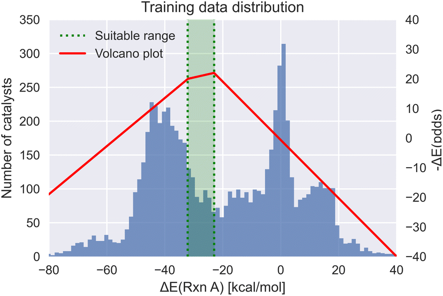 | ||
| Fig. 1 The volcano plot of the oxidative addition energy (red) with the target energy range (green) and the dataset energy distribution (blue).29 | ||
2.2 Data set
Meyer et al. assembled a database consisting of 25![[thin space (1/6-em)]](https://www.rsc.org/images/entities/char_2009.gif) 116 transition metal complexes as reported in ref. 29. This was achieved by combining 91 ligands Lx with six transition metals M (Ni, Pd, Pt, Cu, Ag, and Au) with the L1–M–L2 structural motif (where L1–M–L2 is identical to L2–M–L1). The ligands were chosen to cover the most commonly used chemical groups for Suzuki cross-coupling ligands. Meyer et al. used DFT to compute the binding energies for a selected subset consisting of 7054 catalyst structures (see ESI Fig. S.1 for details†). They used this subset to train and validate their ML approach. The remaining 18064 catalysts that were screened for their suitability have only ML estimated energies associated with them. We used only 7054 molecules and their DFT energy to train, validate and test our generative models. The remaining 18064 catalytic complexes were excluded from the current study. The subset was mostly characterized by Pd metal complexes (2595 complexes), with the remaining 4459 structures distributed among five other transition metals (Pt, Ag, Au, Cu and Ni).
116 transition metal complexes as reported in ref. 29. This was achieved by combining 91 ligands Lx with six transition metals M (Ni, Pd, Pt, Cu, Ag, and Au) with the L1–M–L2 structural motif (where L1–M–L2 is identical to L2–M–L1). The ligands were chosen to cover the most commonly used chemical groups for Suzuki cross-coupling ligands. Meyer et al. used DFT to compute the binding energies for a selected subset consisting of 7054 catalyst structures (see ESI Fig. S.1 for details†). They used this subset to train and validate their ML approach. The remaining 18064 catalysts that were screened for their suitability have only ML estimated energies associated with them. We used only 7054 molecules and their DFT energy to train, validate and test our generative models. The remaining 18064 catalytic complexes were excluded from the current study. The subset was mostly characterized by Pd metal complexes (2595 complexes), with the remaining 4459 structures distributed among five other transition metals (Pt, Ag, Au, Cu and Ni).
2.3 Molecular representation
We used both SMILES33 and SELFIES24 line notations to represent catalyst molecules. The former is a widely adopted representation in cheminformatics and the latter is a recently developed string representation for molecules that, in contrast to SMILES, guarantees that every string corresponds to a valid molecule. SELFIES should have, at least theoretically, a substantial advantage over SMILES since every sequence of SELFIES tokens is guaranteed to correspond to a chemically valid molecule. The two ligands and metal center were represented as individual molecules and separated by the commonly used “.” token. Additionally, a few research groups34,35 demonstrated the benefit of augmenting string representations for improving the predictive performance. Since two different SMILES or SELFIES strings can represent the same molecule, we can leverage the different representations of the same molecules as training augmentation strategies. The augmentation is performed with the RDKit36 function MolToSmiles(doRandom = True). Each of the two ligand molecules is converted into a random SMILES string and afterward assembled back to form an augmented catalyst. This random generation can be done n times for the same molecule, which leads to what we call “n-augmentation” for each catalyst in the training data. The conversion of these augmented catalysts SMILES into SELFIES will also form augmented SELFIES. The SMILES and SELFIES of the catalysts were augmented 0, 8, and 16 times to build 6 data sets. It should be noted that the data augmentation step is done after splitting the data into training and testing sets to guarantee a fair evaluation of a model's performance.2.4 Machine learning architecture
Our VAE19 architecture is made out of three neural networks: an encoder, a decoder, and a property prediction model (see Fig. 2). The encoder is made of recurrent neural network cells and takes the tokenized input representation (i.e. SMILES or SELFIES) and condenses it into an embedding space of smaller size, often referred to as latent space dlatent. The decoder acts on the compressed representation to reconstruct the original inputted sequence. The third model, the property predictor, takes the latent space as an input and is a feed-forward neural network that predicts the target property, in our case the reaction energy. A more detailed description of the architecture can be found in ESI Fig. S.4.† All three models are trained simultaneously. By forcing the input data through this latent space bottleneck, the data are compressed. Furthermore, the simultaneous embedding of the target reaction energy leads to a reorganization of the latent space. The conversion of a discrete input molecule representation into a continuous latent space allows the use of gradient-based optimization procedures for searching the latent space to generate new catalyst candidates.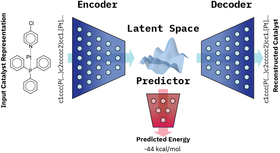 | ||
| Fig. 2 VAE architecture made of three models: an encoder which condenses the inputted catalyst representation into the latent space, a decoder which reconstructs the representation from the latent space and a property predictor which predicts the energy from the latent space. | ||
The training objective of a VAE19 differs from standard autoencoders in the added Kullback–Leibler Divergence (KLD) loss term to regularize the latent space. It minimizes the KL divergence between the approximate posterior and the standard normal distribution  . The overall evidence lower bound (ELBO), which is the training objective, is:
 | (1) |
The first term is the reconstruction loss of the decoder [logPθ(x|z)] representing the reconstruction from the latent variable z and is parameterized by θ. The second term is the KLD between the encoder output (parameterized by ϕ) and a standard normal distribution, DKL(qφ(z|x)∥p(z)) . This loss is scaled by a variable β according to the literature37 from β = 0 to β = 0.1 over 100 epochs. We added to the general VAE ELBO loss, the mean square error of the property prediction model.
3 Results & discussion
3.1 Reconstruction and predictive performance
The training on the original dataset of 7054 catalysts was done by performing a random 90% vs. 10% split. The molecules were tokenized, and the models were trained for 300 epochs with a batch size of 200. The checkpoint used to evaluate the model was the epoch with the lowest validation error. We report more details on training progression in ESI Fig. S.4.† To benchmark our approach ability to predict the oxidative energy for each dataset (0, 8, and 16 augmented SELFIES or SMILES) a VAE with a predictor was trained simultaneously. As seen in Table 1, the best performing model regarding the predictive ability is the VAE trained on the non-augmented SELFIES. With a mean absolute error (MAE) of 2.42 kcal mol−1, it surpasses the two best performing models of the original publication, which are based on the Bag of Bonds (BoB)38 and Spectrum of London and Axilrod–Teller–Muto potential (SLATM)39 representations of molecules (MAE is 2.61 kcal mol−1 and 2.73 kcal mol−1 respectively). Additionally to the VAE, a benchmark random forest with a Morgan fingerprint representation of the catalyst was trained and achieved a performance of MAE = 2.87 kcal mol−1 (see ESI Fig. S.8†). This demonstrates that a string-based representation is sufficient to learn the underlying energy prediction better than the original 3D representations.| Representation | Aug | Validity [%] | Novelty [%] | Predictor MAE [kcal mol−1] | Predictor MSE [kcal mol−1] | Predictor max error [kcal mol−1] | Predictor R2 |
|---|---|---|---|---|---|---|---|
| SMILES | 0 | 49.69 | 45.54 | 2.43 | 14.83 | 26.02 | 0.974 |
| SMILES | 8 | 30.85 | 75.42 | 2.48 | 15.84 | 34.14 | 0.972 |
| SMILES | 16 | 31.91 | 73.71 | 2.73 | 18.11 | 32.34 | 0.968 |
| SELFIES | 0 | 90.86 | 63.87 | 2.42 | 15.02 | 30.28 | 0.973 |
| SELFIES | 8 | 88.94 | 94.49 | 2.53 | 16.49 | 35.68 | 0.971 |
| SELFIES | 16 | 90.22 | 94.00 | 2.73 | 18.43 | 32.70 | 0.967 |
3.2 Latent space organization
We encoded the entire data set into its latent representation to investigate the effect of the predictor neural network on the structure of latent space. Principal component analysis (PCA) was used to better understand and visualize the latent space. The same data set (SMILES 0 augmentation) was used to train two different VAE models, differing in the status (activated/deactivated) of the property predictor neural network. The PCA was done to reduce the dimensionality from the original 32 dimensions to the first two principal components for ease of plotting on a 2D graph (see Fig. 3). The color encoding of each data point with its corresponding energy value reveals visually a clear trend in the latent space. Fig. 3 shows that the model with an active predictor groups together catalysts with similar energy values compared to the one without. We calculate the absolute energy difference, as well as the Euclidean distance in the latent space (see eqn (2)) between each point according to the formula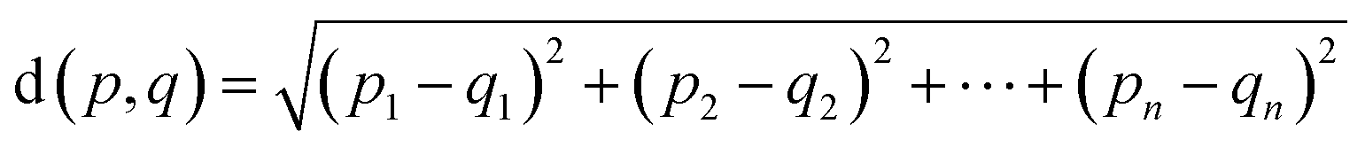 | (2) |
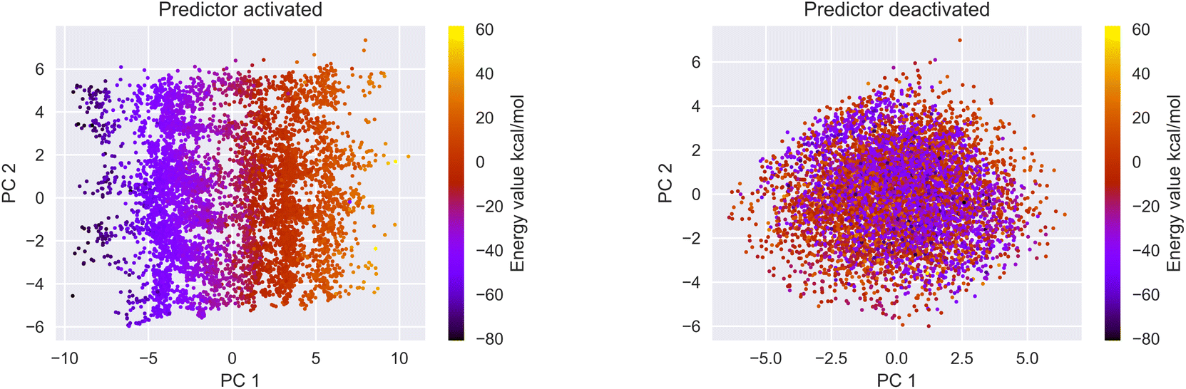 | ||
| Fig. 3 If the predictor is activated (left) the PCA of the latent space reveals a trend from right to left based on the energy values while the model without a predictor (right) is not structured based on the energy values. | ||
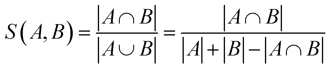
The addition of the property prediction models improves the correlation from 0.02 to 0.69 and therefore will align two points with similar binding energies in a similar region of the latent space. The model with no predictor aligns the molecules depending on their chemical nature in general and will group together chemically similar molecules. To prove this concept, the Morgan fingerprint40 (RDKit36 implementation with a length of 2048 bits was used) of each molecule is computed. This allows the calculation of the Tanimoto similarity metrics (eqn (3)), a commonly used metric to describe how similar a molecule is in its chemical nature:
 | (3) |
We calculated the Euclidean distance and the Tanimoto similarity between each combination of points. The average chemical similarity between all catalysts in the data set is 0.16, while the average chemical similarity between the 10 closest neighbors of each point in the latent space is 0.55 for the model with a predictor and 0.59 for the model without. This result indicates that the models learn to group chemically similar molecules in the latent space.
To evaluate the information density in the latent space, we calculated the Shannon information entropy of each dimension.41 The concept, introduced into generative models by Dollar et al.,42 can be used to investigate if any of the latent dimensions suffers from a posterior collapse, which would correspond to an average entropy value of 0. In such a case, a model learned to ignore this dimension for storing information about molecules. The reconstruction loss term would be ignored and the model aligns this dimension to a normal distribution which satisfies the KLD loss term. ESI Fig. S.11† shows that in every trained model all dimensions are meaningful.
3.3 Generation of molecules
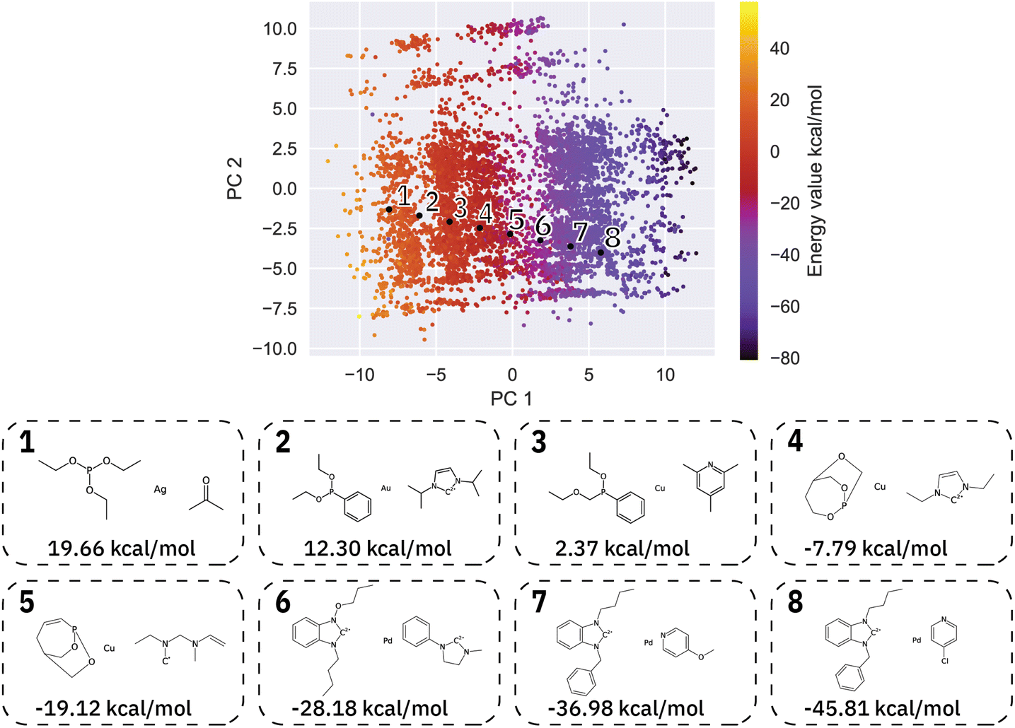 | ||
| Fig. 4 Spacing between two specified molecules (1 and 8) leads to a transformation of the ligands and the metal center. The shift from the metal center from Ag to Pd can be seen. All the points 2–7 are novel generated catalysts not found in the training data. | ||
 and has a learning rate of 0.2. We generated 100 molecules with the objective to select an appropriate number of optimization steps. On average the optimizer already reaches a loss of ypredict = 1.21 ± 0.95 kcal mol−1 in 10 steps which is sufficient to guarantee that all generated molecules lay in the plateau region of the volcano plot, as seen in Fig. 5. The combined training of the predictor model with the VAEs and the resulting structuring of the latent space are beneficial to optimization. When compared to a model where the predictor was trained separately from the VAE (see ESI Fig. S.12†), we can see that the simultaneously trained model requires significantly fewer optimization steps and has a lower standard deviation.
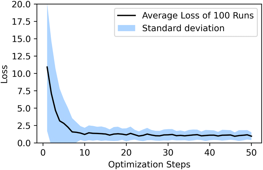 | ||
| Fig. 5 Over one hundred generated molecules, the optimizer reaches an acceptable loss in ten steps. | ||
We then generated 10000 molecules using all SMILES as well as the SELFIES models. We analyzed the generated catalysts for their validity and their novelty or prior existence in the training data. For the exact methodology, we refer to ESI Fig. S.7.† It can be seen that all SELFIES models have a comparatively higher validity as expected by the inherent design of the SELFIES languages. To be a valid molecule, a generated sequence requires two ligands (both valid based on RDKit36 chemical validity) and exactly one metal center. In rare occasions, the SELFIES VAE generates a sequence containing only padding tokens, duplicate metal centers or with one ligand only. This explains a validity lower than 100% in the generated SELFIES. The generated catalysts of the best performing (highest novelty) SELFIES and SMILES models were analyzed. Their chemical structures were inspected to identify the presence of certain functional groups: phosphine, N-heterocyclic carbene and pyridine, selected by popularity in the training data. The analysis revealed that the best suited functional group is phosphine followed by pyridine for both the SELFIES model (see Fig. 7) and SMILES model (see ESI Fig. S.14†) In terms of transition metals, the optimizer favors Pd metal reflecting the same distribution as the training data. Group 11 metals in the periodic table overall tend to be weakly binding, especially in the case of Ag and Au metal complexes. Nevertheless our model can efficiently generate Cu-based catalyst candidates, which are promising leads for more earth-abundant Suzuki catalysts. We report in Fig. 6B a few examples of Cu-based designed catalysts. The analysis of functional group fractions for each metal indicates a distinct preference for phosphine ligands, particularly in the case of Pt, Pd, and Cu based complexes (as shown in Fig. 6A). Additionally, pyridine ligands are also found to be favored, albeit to a lesser extent than phosphine ligands. It should be noted that models suffer also from some limitations such as generating non-novel molecules or chemically valid molecules that are most likely not synthesizable. Another limitation is that the model only considers the catalyst itself, it doesn't include any assumptions about the reaction conditions (such as solvent, bases, additives, temperature), which play a key role in the catalytic activity of the Suzuki-coupling. The fact that we don't encode the binding site implicitly can lead to a non-determined binding site in generated molecules since multiple functional groups acting as binding sites can be present. Even with these limitations we believe that the generative capabilities of these models are a powerful addition to the toolbox of chemists to find new catalysts. All models have been made publicly available through a new generative model library (GT4SD) that eases the training and use even for non-experts.
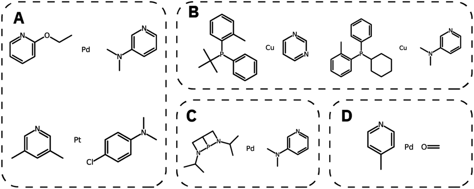 | ||
| Fig. 6 Generated catalyst candidates: (A) pyridine based ligands in combination with the precious metals Pt and Pd and (B) a selection of Cu based catalysts with phosphine and pyridine based ligands. (C) An example for a valid but most likely not synthesizable molecule and (D) a non-novel generated molecule which is part of the training data. | ||
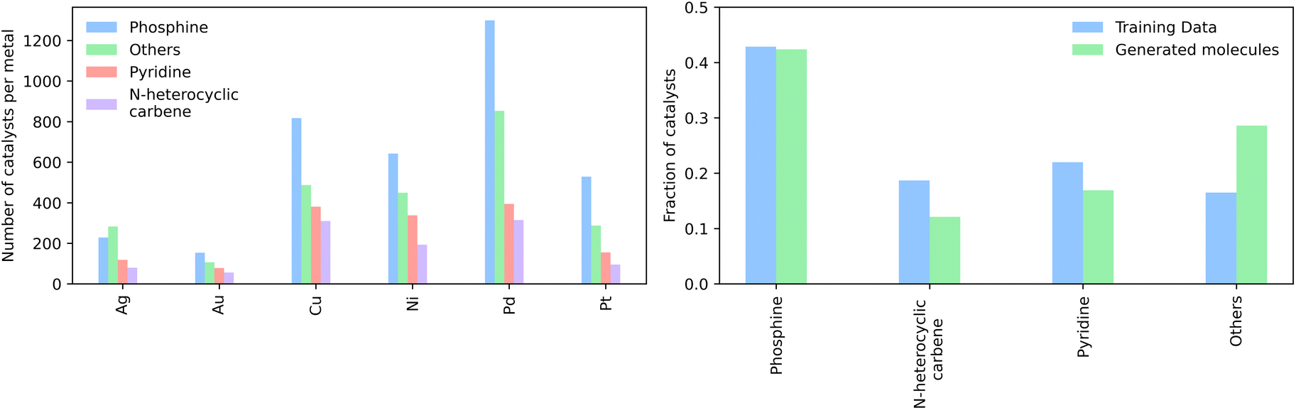 | ||
| Fig. 7 (Left) The distribution of the functional groups in the SELFIES model, where phosphines are the dominant functional group and (right) the number of generated functional groups in the generated molecules of each metal individually. | ||
4 Conclusions
Using a recurrent neural network-based Variational Autoencoder (VAE) and a feed-forward neural network, we demonstrated that string-based catalysts' representations outperform 3D descriptors in the generation of new catalyst ligands with oxidative binding energies deemed suitable for Suzuki cross-coupling reactions. We identified by dimensionality reduction, correlation, and entropy calculations that the latent space is meaningfully organized and does not contain any unused dimensions. We explored the latent space built on SELFIES with the use of gradient-based techniques, generating over 8574 out of 10000 novel and valid catalysts. All models are made available through a generative model library (GT4SD) that will simplify training and use for non-experts, with the hope that this work will facilitate the replacement of more sustainable materials in current catalytic processes.
Data availability
This study was carried out using publicly available data from https://doi.org/10.24435/materialscloud:2018.0014/v1 and https://doi.org/10.24435/materialscloud:2019.0007/v3. The code for all models and plots can be found at https://github.com/GT4SD/gt4sd-core. The version of the code employed for this study is version v0.58.0.Conflicts of interest
There are no conflicts to declare.Acknowledgements
This publication was created as part of NCCR Catalysis (grant number 180544), a National Centre of Competence in Research funded by the Swiss National Science Foundation.Notes and references
- L. K. Mannepalli, C. Gadipelly, G. Deshmukh, P. Likhar and S. Pottabathula, Bull. Chem. Soc. Jpn., 2020, 93, 355–372 CrossRef CAS.
- R. Martin and S. L. Buchwald, Accounts of chemical research, 2008, 41, 1461–1473 CrossRef CAS PubMed.
- B. Sanchez-Lengeling and A. Aspuru-Guzik, Science, 2018, 361, 360–365 CrossRef CAS PubMed.
- D. T. Ahneman, J. G. Estrada, S. Lin, S. D. Dreher and A. G. Doyle, Science, 2018, 360, 186–190 CrossRef CAS PubMed.
- D. W. Robbins and J. F. Hartwig, Science, 2011, 333, 1423–1427 CrossRef CAS PubMed.
- R. Gómez-Bombarelli, J. N. Wei, D. Duvenaud, J. M. Hernández-Lobato, B. Sánchez-Lengeling, D. Sheberla, J. Aguilera-Iparraguirre, T. D. Hirzel, R. P. Adams and A. Aspuru-Guzik, ACS Cent. Sci., 2018, 4, 268–276 CrossRef PubMed.
- A. Gimeno, M. J. Ojeda-Montes, S. Tomás-Hernández, A. Cereto-Massagué, R. Beltrán-Debón, M. Mulero, G. Pujadas and S. Garcia-Vallvé, Int. J. Mol. Sci., 2019, 20, 1375 CrossRef CAS PubMed.
- P. Schwaller, T. Laino, T. Gaudin, P. Bolgar, C. A. Hunter, C. Bekas and A. A. Lee, ACS Cent. Sci., 2019, 5, 1572–1583 CrossRef CAS PubMed.
- P. Schwaller, R. Petraglia, V. Zullo, V. H. Nair, R. A. Haeuselmann, R. Pisoni, C. Bekas, A. Iuliano and T. Laino, Chem. Sci., 2020, 11, 3316–3325 RSC.
- V. R. Somnath, C. Bunne, C. W. Coley, A. Krause and R. Barzilay, Learning Graph Models for Retrosynthesis Prediction, arXiv, 2020, preprint, arXiv:2006.07038, DOI:10.48550/arXiv.2006.07038.
- C. W. Coley, L. Rogers, W. H. Green and K. F. Jensen, ACS Cent. Sci., 2017, 3, 1237–1245 CrossRef CAS PubMed.
- P. Schwaller, R. Petraglia, V. Zullo, V. H. Nair, R. A. Haeuselmann, R. Pisoni, C. Bekas, A. Iuliano and T. Laino, Chem. Sci., 2020, 11, 3316–3325 RSC.
- S. Genheden, A. Thakkar, V. Chadimová, J.-L. Reymond, O. Engkvist and E. Bjerrum, J. Cheminf., 2020, 12, 70 Search PubMed.
- M. H. Segler, M. Preuss and M. P. Waller, Nature, 2018, 555, 604–610 CrossRef CAS PubMed.
- A. C. Vaucher, P. Schwaller, J. Geluykens, V. H. Nair, A. Iuliano and T. Laino, Nat. Commun., 2021, 12, 1–11 CrossRef PubMed.
- A. C. Vaucher, F. Zipoli, J. Geluykens, V. H. Nair, P. Schwaller and T. Laino, Nat. Commun., 2020, 11, 1–11 CrossRef PubMed.
- A. Toniato, P. Schwaller, A. Cardinale, J. Geluykens and T. Laino, Nat. Mach. Intell., 2021, 3, 485–494 CrossRef.
- P. Schwaller, B. Hoover, J.-L. Reymond, H. Strobelt and T. Laino, Sci. Adv., 2021, 7, eabe4166 CrossRef PubMed.
- D. P. Kingma and M. Welling, Auto-Encoding Variational Bayes, arXiv, 2013, preprint, arXiv:1312.6114, DOI:10.48550/arXiv.1312.6114.
- I. J. Goodfellow, J. Pouget-Abadie, M. Mirza, B. Xu, D. Warde-Farley, S. Ozair, A. Courville and Y. Bengio, Generative Adversarial Networks, arXiv, 2014, preprint, arXiv:1406.2661, DOI:10.48550/arXiv.1406.2661.
- D. J. Rezende and S. Mohamed, Variational Inference with Normalizing Flows, arXiv, 2015, preprint, arXiv:1505.05770, DOI:10.48550/arXiv.1505.05770.
- W. Jin, R. Barzilay and T. Jaakkola, International conference on machine learning, 2018, pp. 2323–2332 Search PubMed.
- M. J. Kusner, B. Paige and J. M. Hernández-Lobato, Grammar Variational Autoencoder, arXiv, 2017, preprint, arXiv1703.01925, DOI:10.48550/arXiv.1703.01925.
- M. Krenn, F. Häse, A. Nigam, P. Friederich and A. Aspuru-Guzik, Mach. learn.: sci. technol., 2020, 1, 045024 Search PubMed.
- C. Ates, F. Karwan, M. Okraschevski, R. Koch and H.-J. Bauer, Energy and AI, 2023, 12, 100216 CrossRef.
- A. F. Zahrt, J. J. Henle, B. T. Rose, Y. Wang, W. T. Darrow and S. E. Denmark, Science, 2019, 363, eaau5631 CrossRef CAS PubMed.
- P. Friederich, G. dos Passos Gomes, R. De Bin, A. Aspuru-Guzik and D. Balcells, Chem. Sci., 2020, 11, 4584–4601 RSC.
- R. Laplaza, S. Gallarati and C. Corminboeuf, Chem.: Methods, 2022, e202100107 CAS.
- B. Meyer, B. Sawatlon, S. Heinen, O. A. von Lilienfeld and C. Corminboeuf, Chem. Sci., 2018, 9, 7069–7077 RSC.
- M. D. Wodrich, B. Sawatlon, M. Busch and C. Corminboeuf, Acc. Chem. Res., 2021, 54, 1107–1117 CrossRef CAS PubMed.
- M. Foscato and V. R. Jensen, ACS Catal., 2020, 10, 2354–2377 CrossRef CAS.
- J. G. Freeze, H. R. Kelly and V. S. Batista, Chem. Rev., 2019, 119, 6595–6612 CrossRef CAS PubMed.
- D. Weininger, J. Chem. Inf. Comput. Sci., 1988, 28, 31–36 CrossRef CAS.
- E. J. Bjerrum, SMILES Enumeration as Data Augmentation for Neural Network Modeling of Molecules, arXiv, 2017, preprint, arXiv:1703.07076, DOI:10.48550/arXiv.1703.07076.
- P. Schwaller, A. C. Vaucher, T. Laino and J.-L. Reymond, Mach. learn.: sci. technol., 2021, 2, 015016 Search PubMed.
- G. Landrum, 2022.
- M. Fil, M. Mesinovic, M. Morris and J. Wildberger, Beta-VAE Reproducibility: Challenges and Extensions, arXiv, 2021, preprint, arXiv:2112.14278, DOI:10.48550/arXiv.2112.14278.
- K. Hansen, F. Biegler, R. Ramakrishnan, W. Pronobis, O. A. Von Lilienfeld, K.-R. Muller and A. Tkatchenko, J. Phys. Chem. Lett., 2015, 6, 2326–2331 CrossRef CAS PubMed.
- B. Huang and O. A. von Lilienfeld, Quantum machine learning using atom-in-molecule-based fragments selected on-the-fly, arXiv, 2017, preprint, arXiv:1707.04146, DOI:10.48550/arXiv.1707.04146.
- D. Rogers and M. Hahn, J. Chem. Inf. Model., 2010, 50, 742–754 CrossRef CAS PubMed.
- C. E. Shannon, Bell Syst. Tech. J., 1948, 27, 379–423 CrossRef.
- O. Dollar, N. Joshi, D. A. C. Beck and J. Pfaendtner, Chem. Sci., 2021, 12, 8362–8372 RSC.
- A. Paszke, S. Gross, F. Massa, A. Lerer, J. Bradbury, G. Chanan, T. Killeen, Z. Lin, N. Gimelshein, L. Antiga, A. Desmaison, A. Kopf, E. Yang, Z. DeVito, M. Raison, A. Tejani, S. Chilamkurthy, B. Steiner, L. Fang, J. Bai and S. Chintala, arXiv, 2019, preprint, arXiv:1912.01703, DOI:10.48550/arXiv.1912.01703.
Footnotes |
| † Electronic supplementary information (ESI) available. See DOI: https://doi.org/10.1039/d2dd00125j |
| ‡ Current address: EPFL Lausanne, Rte Cantonale, 1015 Lausanne, Switzerland. |
| This journal is © The Royal Society of Chemistry 2023 |