
 Open Access Article
 This Open Access Article is licensed under a Creative Commons Attribution-Non Commercial 3.0 Unported Licence
FEFOS: a method to derive oxide formation energies from oxidation states†
Michael John
Craig
 *ab,
Felix
Kleuker
a,
Michal
Bajdich
*b and
Max
García-Melchor
*a
*ab,
Felix
Kleuker
a,
Michal
Bajdich
*b and
Max
García-Melchor
*a
aSchool of Chemistry, CRANN and AMBER Research Centres, Trinity College Dublin, College Green, Dublin 2, Ireland. E-mail: craigmi@tcd.ie; garciamm@tcd.ie
bSUNCAT Center for Interface Science and Catalysis, SLAC National Accelerator Laboratory, Menlo Park, California 94025, USA. E-mail: bajdich@slac.stanford.edu
First published on 8th May 2023
Abstract
Herein we report a method to extract formation energies from oxidation states, which we call FEFOS. This new scheme predicts the formation energies of binary oxides through analyzing unary oxide formation energies as a function of their oxidation states. Taking averages of fitted quadratic equations that represent how elements respond to oxidation and reduction, the weights of these averages are determined by constraining the compound to be neutral. The application of FEFOS results in mean absolute errors of ca. 0.10 eV per atom when tested against Materials Project data for oxides with general formulas A1−zBzO, A1−zBzO1.5, and A1−zBzO2 with specific coordinations. Our FEFOS method not only allows for the prediction of binary oxide formation energies with low variance and high interpretability, but also compares well with state-of-the-art deep learning methods without being biased by training data and the need for large resources to compute it. Finally, we discuss the potential applications of the FEFOS method in tackling the problem of inverse catalyst design.
Introduction
In 2011, the Materials Genome Initiative was announced by the National Science and Technology Council, an executive branch of the United States Government. This initiative hailed hundreds of millions of dollars of research and development investment into the accelerating materials discovery through combining insights from experiment, theory, and computation.1,2 Furthermore, the rate of scientific research output is growing year on year at a rate of 4% leading to a doubling rate roughly every 15 years.3 With such a spate of data, machine learning algorithms tackle this by attempting to ‘learn’ materials descriptors based on available training data. The state-of-the-art in this area is a method which uses deep learning (DL) to allow for structure-agnostic forecast of materials formation energies, and represents any material composition as a graph where nodes in the graph are weighted by composition.4,5 This approach, referred to as Representation Learning from Stoichiometry (or Roost), achieved a mean absolute error (MAE) of 0.03 eV per atom on a test set of formation energies.4 These methods come with drawbacks, however, since they are difficult to interpret by inspecting the weights of large neural networks (NNs) which have on the order of millions of parameters. Recent evidence also indicates that interpreting these models for domain knowledge is not viable. In addition, Sparks and co-workers showed that training NNs on a random featurization of elemental properties is as performant as using chemical properties in the limit of large data, indicating that the models are not ‘learning’ any chemical or physical concepts.6The notion of an oxidation state (OS) dates back to 1835 when Wohler described elements which can form different oxides.7 It has since seen widespread use as a useful chemical concept to describe chemical bonding and elemental charge in compounds. How this quantity relates to other chemical notions such as covalency or ionicity remains controversial,8–10 even so, the notion of the formal oxidation state is a powerful and prominent concept in chemistry.
In this work, we develop a simple scheme to derive formation energies from oxidation states (FEFOS) to forecast standard formation energies of binary oxides from the Materials Project (MP) database,11 and compare our predictions to the Roost method. This approach takes a well-known phenomenon in solid oxide chemistry – namely, that cations in binary oxides balance their respective charges to their preferred oxidation states – and uses this knowledge to derive a model for the enthalpy of formation of binary oxides based on the enthalpy of formation of unary oxides. Notably, the FEFOS method only requires two parabolas per element and oxide stoichiometry, leading to an interpretable, extensible method with comparable errors to those shown by the state-of-the-art DL approach implemented in Roost. The physical implication of this is that a primary driving force towards the formation of binary oxides lies in the balancing of charges. Furthermore, the interpretability of FEFOS is demonstrated by describing two distinct cases of alloying SnO2 and NbO2 with earth-abundant elements and relating the performance of our model in terms of the preference of specific elements for a specific OS. Lastly, we present how the FEFOS model could be used to enable inverse design in catalysis, specifically for the oxygen evolution reaction (OER). We envision this new method to inform experiments on the propensity of metal oxides towards mixing, the stability of the resulting oxide(s), as well as the optimal concentration of the constituent elements, thus accelerating inverse catalyst design.
Results
The FEFOS method
When elements are mixed in oxides, there is often concomitant oxidation and reduction of the respective elements.12–14 To generally describe the propensity of a given element to be oxidized or reduced when mixed, we fit quadratic equations through formation energies at the standard state of the most stable entries (lying on the convex hull) in the MP database across all available M![[thin space (1/6-em)]](https://www.rsc.org/images/entities/char_2009.gif) :O ratios. These oxide formation energies are calculated by MP, which use a chemical potential for oxygen (μO) of −4.95 eV with a correction of −0.687 eV per O atom applied – this value was derived by Wang et al. through comparing calculated formation energies from GGA+U to room temperature experimental formation enthalpies, with the PΔV term neglected15 — and attempts to account for the overbinding of the molecular O2 reference.16 For V, Cr, Mn, Fe, Co, Ni, Mo and W-containing oxides, a composition-weighted correction is also applied to allow for the mixing of GGA and GGA+U-calculated energies.17
:O ratios. These oxide formation energies are calculated by MP, which use a chemical potential for oxygen (μO) of −4.95 eV with a correction of −0.687 eV per O atom applied – this value was derived by Wang et al. through comparing calculated formation energies from GGA+U to room temperature experimental formation enthalpies, with the PΔV term neglected15 — and attempts to account for the overbinding of the molecular O2 reference.16 For V, Cr, Mn, Fe, Co, Ni, Mo and W-containing oxides, a composition-weighted correction is also applied to allow for the mixing of GGA and GGA+U-calculated energies.17
For each element, M, and each oxidation state of interest 2y, we construct two quadratic equations, fox,MOy(x) and fred,MOy(x), which take the general form:
| fox/red,MOy(x) = a1,MOyx2 + a2,MOyx | (1) |
 , or for AaBbOc,
  . Note that we use x as a variable in phase diagram construction to represent the oxidation state shift so that x is derived from composition as in typical convex hull diagrams, but indirectly through our assumed oxidation state.
In Fig. 1a we fit the above quadratic equations over the standard formation energies for the oxidation of Mo, fox,MoO2(x) = 0.022x2 + 0.003x, and the reduction of Cr, fred,CrO2(x) = 0.319x2 − 0.638x, where we use CrO2 and MoO2 as our (0, 0) point and fit through the points which we define as the convex hull in the direction of oxidation or reduction. Given Cr2O3 is the chromium-based oxide with the lowest formation energy, this curve is a mathematical representation of the fact that Cr′s preferred OS is 3+ and is symmetric about this point so that the y-axis is zero (i.e. the same as CrO2) for OS 2+. On the other hand, the fox,MoO2(x) parabola is very shallow and concave, having been fitted through Mo8O23 and MoO3.
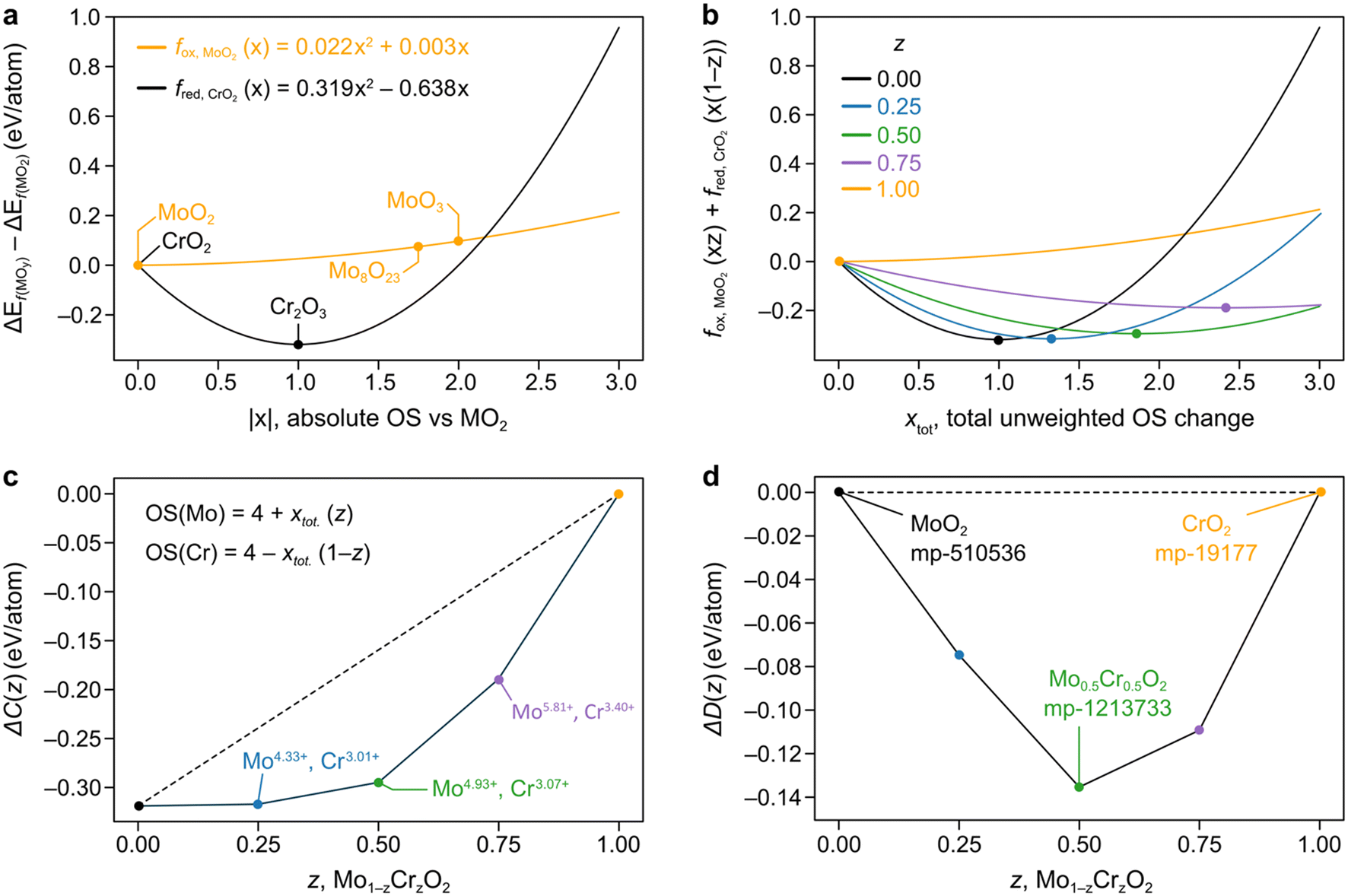 | ||
Fig. 1 a) Parabolas for the reduction of Cr and the oxidation of Mo formed by fitting through ground state oxides found in MP, with fitted datapoints indicated by the stoichiometry of the material. The x-axis represents the absolute OS change with respect to the reference MO2 oxide (|x|). Recall that for an oxide AaOc, we have that  . b) Weighted averages of the two curves from a), dependent on the concentrations of Cr and Mo, z, with the minima of these curves denoting ΔC(Mo1−zCrzO2) as in eqn (3). The x-axis here represents the overall oxidation state change (xtot.) without being weighted by concentration. c) Representation of the minima of the curves plotted in b) as a function of z. The approximated oxidation states of each element derived by taking the product of xtot. and the relevant concentration are also shown. The dashed line is to guide the eye connecting the values for z = 0, 1. d) Convex hull phase diagram constructed using ΔD(A1−zBzO2) from eqn (5) and (6) and compared against calculations found in the MP database. . b) Weighted averages of the two curves from a), dependent on the concentrations of Cr and Mo, z, with the minima of these curves denoting ΔC(Mo1−zCrzO2) as in eqn (3). The x-axis here represents the overall oxidation state change (xtot.) without being weighted by concentration. c) Representation of the minima of the curves plotted in b) as a function of z. The approximated oxidation states of each element derived by taking the product of xtot. and the relevant concentration are also shown. The dashed line is to guide the eye connecting the values for z = 0, 1. d) Convex hull phase diagram constructed using ΔD(A1−zBzO2) from eqn (5) and (6) and compared against calculations found in the MP database. | ||
The general idea is to combine the above quadratic equations to represent binary formation energies in the restricted composition space of Mo1−zCrzO2 with {z ∈ R| 0 ≤ z ≤ 1}. To maintain charge balance, we constrain the average OS of any material AaBbOc to be  . We then enforce that the mixed compositions have the same fixed average OS as the initial pure oxides, e.g. in the case of MO2-type oxides this OS is 4+. If we now use o and r to represent the oxidation and reduction of a material A1−zBzOy, (where y = {1, 1.5, 2}) to keep the OS constant when mixing we need:
| o(1 − z) − rz = 0, | (2) |
For instance, a Sb0.67Ni0.33O2 could exhibit Sb5+ and Ni2+ under this scheme, so that the overall OS remains 4+. In real systems, however, such ideal oxidation mixing eventually breaks down, and further compensation occurs via formation of defects, i.e. oxygen and metal vacancies.18 Yet, as we demonstrate in the following, our scheme is sufficient to forecast binary oxide formation energies at fixed stoichiometries.
To mathematically define a combination energy, ΔC, we use the quadratic equations fox,AOy(x), fred,AOy(x), fox,BOy(x), and fred,BOy(x) for a hypothetical material A1−zBzOy. These are used to test both combinations of oxidizing and reducing either of the constituent elements, and by minimizing these curves we arrive to:
| ΔC = minx(fox,AOy(xz) + fred,BOy(x(1 − z)), |
| fred,AOy(x(1 − z)) + fox,BOy(xz)) | (3) |
Then, to represent a mixing formation energy with respect to segregation against CrO2 and MoO2, we define ΔD(A1−zBzOy) with:
| ΔD(A1−zBzOy) = 0 for z = {0, 1} | (4) |
| ΔD(A1−zBzOy) = ΔC(A1−zBzOy) − (1 − z)ΔC(A1B0Oy) − zΔC(A0B1Oy) | (5) |
| ΔEf(A1−zBzOy) ∼ ΔD(A1−zBzOy) + (1 − z)ΔEf(AOy) + zΔEf(BOy) | (6) |
We demonstrate the application of this method to predict ΔD(A1−zBzOy) for mixing Cr and Mo in the MO2 stoichiometry, as seen in the convex hull phase diagram constrained to the Mo1−zCrzO2 phase space in Fig. 1d. Importantly, we observe almost no deviation between our prediction and the observed Mo0.5Cr0.5O2 material in the MP database (ID mp-1213733). Therefore, our FEFOS method holds promise as a rapid means of garnering a forecast for the minimum energy over a span of concentrations for a given stoichiometry, as well as the OS of the respective elements. In the case outlined in Fig. 1, we can read off the predicted OS of Cr and Mo by noting the value of x which minimizes the curves in Fig. 1b and multiplying that value by the concentration of the other element. For example, we see that for z = 0.5, the minimum weighted average in eqn (3) is for xtot. = 1.86. Multiplying this change by z gives that the change in OS should be 0.93 relative to the MO2 unary oxide. Therefore Cr and Mo should have OS values of 3.07 and 4.93, respectively; such non-integral values for OS have been previously proposed to be observable.19
We now gather quadratic equations for elements across the periodic table and compare our approximated ΔEf to the values reported by MP for any binary oxide which is composed of elements within the considered set and with an M:O ratio of 1:2, 1:1.5 and 1:1. The method used to construct these parabolas and their coefficients, as in eqn (1), for each considered element can be found in the ESI.†
Benchmark of the FEFOS method
Using eqn (6), we now approximate ΔEf using ΔD for a series of binary oxides with general formula A1−zBzO2, A1−zBzO1.5, and A1−zBzO, where z = [0–1]. This requires 6 quadratic equations per element, A or B, representing both oxidation and reduction from the reference unary oxides AO2, A2O3, and AO. We then select the following set of elements found in oxides of the three aforementioned types in the MP database, i.e. Ag, Al, As, Au, Ba, Be, Bi, Br, Ca, Cd, Ce, Co, Cr, Cs, Cu, Dy, Er, Eu, Fe, Ga, Gd, Ge, Hf, Hg, Ho, In, Ir, K, La, Li, Lu, Mg, Mn, Mo, Na, Nb, Nd, Ni, Os, Pb, Pd, Pr, Pt, Rb, Re, Rh, Ru, Sb, Sc, Se, Si, Sm, Sn, Sr, Ta, Tb, Tc, Te, Ti, Tl, Tm, V, W, Yb, Zn, and Zr.Our FEFOS model is constructed with the notion of a constant average OS across the composition of a binary oxide, so we use a filtering condition which requires: i) A and B are within 2.5 Å to six oxygen atoms, and ii) oxygen atoms are taken to be O2− anions which are within 2.5 Å to 3, 4, or 6 metal atoms, if the binary oxide to be represented is of type A1−zBzO2, A1−zBzO1.5, or A1−zBzO, respectively. If each A and B is octahedral, then the total anionic charge is 12, the overall charge is then 4, 3 or 2 depending on whether there are 3, 4 or 6 metal atoms bound to the A and B atoms. This way we attempt to constrain the overall OS across the elements A and B, where both are elements that exhibit a unique OS for every site in the oxide. The upper bound of 2.5 Å is based on prior studies of metal–oxygen bond length distributions.20 We then gather every MP entry which fit these criteria and compare FEFOS forecasted ΔD(A1−zBzO(1,1.5,2)) values against the MP value.
A parity plot of our predictions for ΔEf(A1−zBzO1.5) against the observed MP is shown in Fig. 2a, where we can see a low error between forecasted and MP-calculated points despite the simplicity of the FEFOS model. MAE values of forecasted and MP-reported formation energies of 0.105 and 0.171 eV per atom are shown for the case where we do and do not filter by coordination, respectively. To highlight the need to filter by coordination, we include the unfiltered cases as pink circles, where we observe a higher error than if we restrict our comparisons to specific coordinations (blue circles). This is expected, since controlling for coordinations should reduce the possibility that each element has distinct OSs, which our model does not represent as it only considers that A and B have constant OSs. To confirm that the remaining structures still represent a diverse set of oxides, in Fig. S1† we have analyzed the distribution of space group numbers in the filtered and unfiltered groups, where we note that while the span of space groups is lower than the unfiltered group, it is not concentrated within any one subset of space groups.
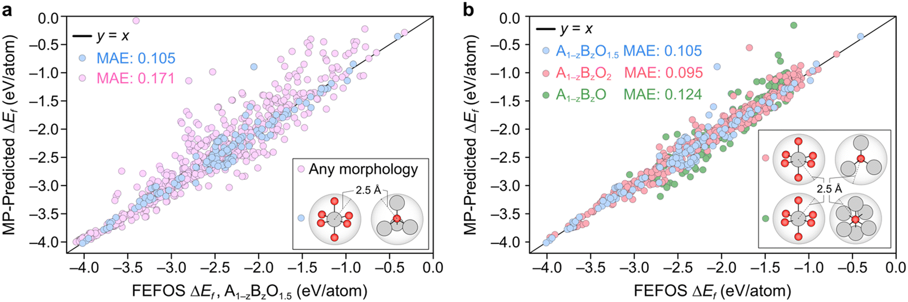 | ||
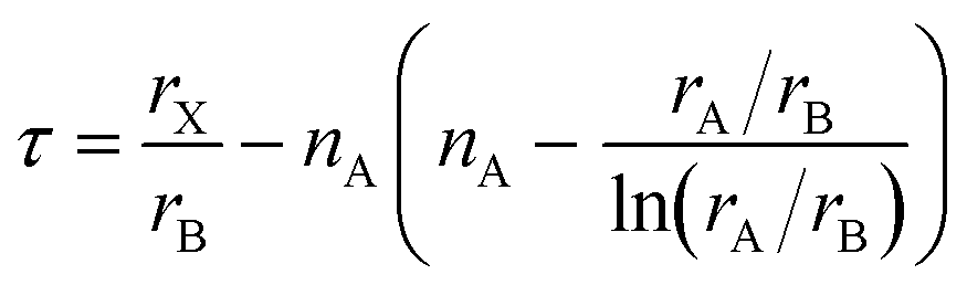
| Fig. 2 a) Parity plot showing the ΔEf values for binary oxides with stoichiometry A1−zBzO1.5 derived from the FEFOS prediction scheme outlined in this work against the MP entries for different sets of filtered and unfiltered data. The blue and pink colors represent filtered and unfiltered structures with formula A1−zBzO1.5 and with the condition shown in the inset. Blue points contain only those structures which are comprised solely of oxides with A and B atoms within 2.5 Å of 6 oxygen atoms, and oxygen atoms within 2.5 Å of 4 A or B atoms. b) Parity plots as in a) including the oxide stoichiometries A1−zBzO1.5 (blue circles), A1−zBzO2 (red circles) and A1−zBzO (green circles), where again we only plot those structures made up of A and B atoms within 2.5 Å of 6 oxygen atoms, and oxygen atoms that are within 2.5 Å of 4, 3, or 6 A or B atoms, respectively. In each case, the line y = x is drawn to guide the eye. Color code of atoms in insets: oxygen (red), metal (grey). | ||
Fig. 2b illustrates the result of including the forecasted ΔEf values against the MP entries where the filtering condition on oxide stoichiometry is applied for each OS. These data include the blue datapoints for A1−zBzO1.5, shown in Fig. 2a, as well as red and green circles for A1−zBzO2 and A1−zBzO oxides, respectively. Here we see comparable MAE values as seen for A1−zBzO1.5 oxides of 0.095 and 0.124 eV per atom for A1−zBzO2 and A1−zBzO oxides, respectively. This underscores the versatility of the FEFOS method described in this work as it can be applied to distinct classes of binary oxides with errors comparable to the best available DL methods. To demonstrate this, in the following we compare the performance of FEFOS to the aforementioned Roost method used to approximate formation energies, which reported a test set of 25663 entries from the Open Quantum Materials Database21 with a MAE of 0.03 eV per atom when trained with 230959 datapoints.4
The developers of Roost thankfully accompanied their report with a spreadsheet of values including the composition, target variable and prediction for each of the 25663 test datapoints, and therefore we can condition the composition so that we only compare values for A1−zBzO(1,1.5,2) oxides. They also provided a learning curve, where they reported the error in their test set when the DL algorithm had been trained on progressively more datapoints. In Fig. 3, we compare both the test MAE across all data to ensure we reproduce the reported value, and the MAE for all oxides of the same type considered by our FEFOS model, showing these values as a function of the number of training datapoints. Notably, the Roost error is higher for oxides we have studied in this work, as may be expected given the higher degree of complexity within this class of materials. In addition, while the error with Roost becomes lower than with FEFOS when the DL algorithm is trained on more than 100000 datapoints from the OQMD,21 our model has far lower complexity and more interpretability.
 | ||
| Fig. 3 Learning curves of the Roost method4 for both the as-reported datapoints (red circles), which include the entire OQMD formation energy test set, and datapoints for OQMD entries which have the form A1−zBzO(1,1.5,2) (blue circles). The overall MAE from our FEFOS method from Fig. 2 is shown as a horizontal dashed line. | ||
Application of FEFOS to SnO2- and NbO2-based alloys
We now demonstrate the applicability of the FEFOS model to a technologically relevant problem, namely the alloying of metal oxides with earth-abundant elements. In particular, in Fig. 4a we present the results of alloying SnO2, where the FEFOS method agrees with MP-calculated energies for first-row transition metals in that it predicts they are unstable with respect to their native SnO2 and BO2 phases. The difficulty in alloying with SnO2 is related to the high stability of tin dioxide and its relatively low formation energy with respect to other competing phases. That is, SnO2 lies at the bottom of the convex hull for the Sn–O composition, which can be noted for the purposes of our model from the equations for fox,SnO2(x) = 0.77x and fred,SnO2(x) = 0.057x2 + 0.12x, which are positive for all x > 0. | ||
| Fig. 4 Constrained convex hull diagrams showing the predicted ΔD from eqn (5) across the compositions spaces a) Sn1−zBzO2 and b) Nb1−zBzO2 after alloying them with earth-abundant elements, B. The datapoints denote MP-calculated values which the FEFOS model attempts to capture. Predictions are plotted across composition space, not only comparing them with MP data, as in Fig. 2. | ||
The elements which show the lowest ΔD(Sn1−zBzO2) at low concentrations (z < 0.1) are Nb and W, which have their lowest formation energies for OSs 5+ and 6+, respectively. We attribute this to the fact that all of the tested 3d elements except Ti are most stable at lower oxygen concentrations than is seen in rutile structures (M:O = 1:2), so their fred,MO2(x) equation must out-compete fox,SnO2(x) = 0.77x. On the other hand, for Nb and W the relevant Sn equation is fred,SnO2(x) = 0.057x2 + 0.12x which exhibits a shallower slope. SnO2 is known to form oxygen vacancies more readily than tin vacancies,22 so this mathematical construction agrees with that observation, as well as a recent paper reporting the doping of SnO2 with Nb, W and Ta for application as a transparent conducting oxide.18 As an aside, we highlight that if ΔD(Sn1−zBzO2) < 0 it implies that the material is stable with respect to segregation to SnO2 and BO2, but not necessarily against segregation to other competing phases.
Unlike SnO2, Fig. 4b shows how doping NbO2 with first-row transition metals result in negative ΔD(Nb1−zBzO2) values due to their preference for reduction with respect to MO2 (excluding Ti). This is accompanied by the lowest formation energy for Nb being seen for Nb2O5, implying that Nb prefers to be oxidized from 4+ to 5+. It is also worth noting that, except for Mn, the positions of the minima of our curves appear to align well with the MP-calculated values (circles), which we could reasonably assume are close to the true minima. For example, the Cu, Co, and Ni points are clustered around the Nb (z = 0.33) region, attributable to these metals' affinity for OS 2+, while Fe and Cr have minima closer to Nb (z = 0.5) due to the ‘preference’ of these metals for OS 3+. In contrast, the second and third-row transition metals Mo and W show positive ΔD(Nb1−zBzO2) values since they are competing against Nb4+ reduction.
Interestingly, we find that for MnNb2O6 (MP ID: mp-22100), an older calculation not indexed by MP, is lower in energy. This appears to be due to a process by which MP does not index calculations with old input settings. In this case, the initialized magnetic moments for the Mn atoms were less than 1μB in the newer calculations compared to 5μB in the old ones, despite the expected high-spin state of Mn2+ ions. Notably, when the older, lower energy is used, the minimum aligns more closely with that forecasted by our FEFOS method, indicating that this tool is also useful in detecting outliers within materials databases, and demonstrating its predictive power. We also note that this calculated material matches an ICSD entry despite MP giving it an energy above hull of 0.25 eV per atom. In fact, if we take the older calculation as the ground truth, the formation energy is lowered by 0.29 eV per atom and it becomes below the hull.
Discussion
The FEFOS method presented in this work is extremely fast, with the ability to generate the predictions shown in Fig. 2 on the order of seconds. Furthermore, the interpretability of the model allows us to make broad statements about OS shifting, with implications across field of materials science and catalysis.In previous work, we showed that the OER descriptor for hypothetical molecular complexes is OS-dependent and that this quantity was not correlated between oxidation states.21,23 Each of these factors are important in thinking about mixing elements at a given M:O ratio with OER catalysis in mind. As shown in Fig. 5a, an ideal scenario for OER would be one whereby A and B elements in AOx and BOx are non-ideal catalysts, but their reduced and oxidised counterparts, respectively, are. This is illustrated in Fig. 5a where A is reduced and B is oxidised by some unspecified degree, and in Fig. 5b we depict a scenario where this leads their OER activity descriptors to get closer to the ideal value. This picture could explain why doping Ir and Ru oxides with elements which have an affinity for OS 3+ or lower improves OER activity,22,24–30 since the OS of Ir and Ru atoms increases. Indeed, computational results have shown that IrO2 and RuO2 have lower OER activity descriptors than the ideal value,31,32 and that when these metals are in a higher OS it approaches the ideal value. Precisely this explanation from first principles calculation was used to justify the activity of low concentration Ir sites hosted in a WO3 oxide.22 Conversely, Sargent et al. have observed that the activity of NiFe and CoFe oxyhydroxides can be improved by doping them with high-valent elements Mo5+, Ta5+, Nb5+, Re6+ or W6+,13 and this enhancement in catalytic rate was justified on the basis that the Fe atoms were reduced relative to the undoped catalysts.
 | ||
| Fig. 5 Scheme illustrating a scenario where two hypothetical elements A and B are reduced and oxidized, respectively, due to their unmixed oxides affinity for lower and higher OS, respectively, compared to that seen in MOx. In the ideal scenario presented here, a) represents the stability shifts upon oxidation state changes, while b) shows how the both A and B exhibit a lower OER overpotential (ηOER) in the AzB1−zOx mixture relative to the unmixed case due to the behaviour of the OS-dependence of the unmixed OER descriptors. | ||
The spate of data in computational materials databases has led to the creation of machine learning-based techniques to forecast formation energies, which have seen some success. However, these methods suffer severe limitations since they require huge amounts of data to become useful and their predictions may be biased towards previously discovered classes of materials. Furthermore, understanding the outputs of machine learning models is challenging. In contrast, the FEFOS model only requires information about unary oxides, thereby allowing for the automatic screening of any potential combination of elements for a given oxygen content. Another advantage of FEFOS is that the source of stabilisation/destabilisation can be easily interpreted with respect to an element's propensity to be oxidised or reduced.
On a related note, the prediction of the stability of perovskites (with general formula ABX3) has relied on the use of the Goldschmidt tolerance factor,20t, defined as:
 | (7) |
 | (8) |
Our method is currently restricted to oxides which contain only octahedral sites. Future work will study whether oxides with mixed coordination numbers could be modelled with FEFOS using coordination-specific parabolic equations and consider the relative affinities for oxidation states in more than one type of coordination (e.g. octahedral and tetrahedral sites in a spinel oxide). The applicability of the FEFOS method to such systems relies on the notion that phase diagram surfaces can be drawn as quadratic equations, but the shape of these surfaces could conceivably be more appropriate as a piecewise linear function, or step functions in the case of p-block elements like Sn, which are only known to exist as Sn2+ or Sn4+. Finally, at low concentrations of dopant, the OS of the host material is only slightly shifted, meaning that the resolution of the phase diagram close to the minimum of the convex hull determines the accuracy of predictions.
Conclusions
In this work we develop and test the FEFOS model which shows similar performance to Roost, a state-of-the-art deep learning method trained on tens of thousands of computational materials datapoints. While we do not study as wide an array of structures, we outline how the FEFOS method can be extended to other M:O ratios by fitting more sets of quadratic equations and is far more interpretable than a black box machine learning method using a vast set of features. By focusing on oxides and OS specifically, a prime source of stability can be explained with respect to which elements are changing their OS in what direction and by what amount. Furthermore, this method could feasibly be extended to other stoichiometries and oxides containing more elements. We expect this approach to facilitate high-throughput screening for materials applications of multicomponent oxides.
Methods
To fit the quadratic equations, unary oxide data for Ag, Al, As, Au, Ba, Be, Bi, Br, Ca, Cd, Ce, Co, Cr, Cs, Cu, Dy, Er, Eu, Fe, Ga, Gd, Ge, Hf, Hg, Ho, In, Ir, K, La, Li, Lu, Mg, Mn, Mo, Na, Nb, Nd, Ni, Os, Pb, Pd, Pr, Pt, Rb, Re, Rh, Ru, Sb, Sc, Se, Si, Sm, Sn, Sr, Ta, Tb, Tc, Te, Ti, Tl, Tm, V, W, Yb, Zn, and Zr was gathered from the Materials Project. Formation energy data required for the analyses were collected using the pymatgen interface (as of the 2022.4.19 release) with the Materials Project API.The pymatgen structure data, coordination data and formation energy data are contained within the binary files unary_data.p, binary_data.p and binary_pairing_data.p within the data_gather folder. To fit the quadratic equations, we set the y-axis as the shift with respect to the reference oxide formation energy for the element unary oxide at each of the relevant oxygen stoichiometries. This reference formation energy was determined to be the oxide with the lowest energy for that element at that stoichiometry. If no such oxide existed in the database, we do not create quadratic equations for that element.
The reference formation energies – where they existed in MP – for each of the 68 elements can be found at: https://github.com/michaelcraiger/fefos/tree/main/supplementary_data in the file named reference_oxides.csv.
The fitted quadratic equations for fox,MO, fred,MO, fox,MO1.5, fred,MO1.5, fox,MO2, and fred,MO2 in eqn (1) for each of the considered elements can be found under the filename parabola_coeffs.csv, which is a spreadsheet containing sheets which each coefficient, as well as separated.csv files with the same data in MO_parabs.csv, M2O3_parabs.csv and MO2_parabs.csv.
All the resultant fitted quadratic equations are plotted along with the associated MP data points for every considered element in the ESI.†
The coefficients were then used to solve eqn (6) such that formation energy predictions for Fig. 2 could be made. The results of each prediction both with and without filtering oxide structure is found under the file fefos_predictions.csv.
To collect Roost test errors for Fig. 3, we collated and parsed the relevant information from ref. 4, with the .csv files contained in the roost_test_data folder of the repository.
Code availability
The code used for this study can be accessed via a link to the public repository https://github.com/michaelcraiger/fefos. Instructions on how to use the code to generate the results are also provided in the above link.Data availability
The datasets required to carry out the analyses reported in the report can be found via the following link to the public repository https://github.com/michaelcraiger/fefos.Author contributions
M. J. C. devised the method and wrote the code and first draft of the manuscript, F. K. reviewed the central concept and code. M. G.-M. and M. B. provided supervision throughout. All authors contributed to writing and revising the manuscript.Conflicts of interest
There are no conflicts to declare.Acknowledgements
We acknowledge the support from the Irish Research Council (GOIPG/2019/2367), Science Foundation Ireland (SFI-20/FFP-P/8740), and the U.S. Department of Energy, Office of Science, Office of Basic Energy Sciences, Chemical Sciences, Geosciences, and Biosciences Division, Catalysis Science Program to the SUNCAT Center for Interface Science and Catalysis.Notes and references
- J. J. de Pablo, B. Jones, C. L. Kovacs, V. Ozolins and A. P. Ramirez, The Materials Genome Initiative, the interplay of experiment, theory and computation, Curr. Opin. Solid State Mater. Sci., 2014, 18, 99–117 CrossRef.
- J. J. de Pablo, et al., New frontiers for the materials genome initiative, npj Comput. Mater., 2019, 5, 41 CrossRef.
- L. Bornmann, R. Haunschild and R. Mutz, Growth rates of modern science: a latent piecewise growth curve approach to model publication numbers from established and new literature databases, Humanit. Soc. Sci. Commun., 2021, 8, 224 CrossRef.
- R. E. A. Goodall and A. A. Lee, Predicting materials properties without crystal structure: deep representation learning from stoichiometry, Nat. Commun., 2020, 11, 6280 CrossRef CAS PubMed.
- C. J. Bartel, et al., A critical examination of compound stability predictions from machine-learned formation energies, npj Comput. Mater., 2020, 6, 97 CrossRef.
- R. J. Murdock, S. K. Kauwe, A. Y.-T. Wang and T. D. Sparks, Is Domain Knowledge Necessary for Machine Learning Materials Properties?, Integr. Mater. Manuf. Innov., 2020, 9, 221–227 CrossRef.
- P. Karen, Oxidation state, a long-standing issue!, Angew. Chem., Int. Ed., 2015, 54, 4716–4726 CrossRef CAS PubMed.
- M. Jansen and U. Wedig, A Piece of the Picture-Misunderstanding of Chemical Concepts, Angew. Chem., Int. Ed., 2008, 47, 10026–10029 CrossRef CAS PubMed.
- A. Walsh, A. A. Sokol, J. Buckeridge, D. O. Scanlon and C. R. A. Catlow, Electron Counting in Solids: Oxidation States, Partial Charges, and Ionicity, J. Phys. Chem. Lett., 2017, 8, 2074–2075 CrossRef CAS PubMed.
- A. Walsh, A. A. Sokol, J. Buckeridge, D. O. Scanlon and C. R. A. Catlow, Oxidation states and ionicity, Nat. Mater., 2018, 17, 958–964 CrossRef CAS PubMed.
- A. Jain, et al., Commentary: The Materials Project: A materials genome approach to accelerating materials innovation, APL Mater., 2013, 1, 011002 CrossRef.
- L. Zhou, et al., Rutile Alloys in the Mn–Sb–O System Stabilize Mn 3+ To Enable Oxygen Evolution in Strong Acid, ACS Catal., 2018, 8, 10938–10948 CrossRef CAS.
- B. Zhang, et al., High-valence metals improve oxygen evolution reaction performance by modulating 3d metal oxidation cycle energetics, Nat. Catal., 2020, 3, 985–992 CrossRef CAS.
- M. J. Craig and M. García-Melchor, Faster hydrogen production in alkaline media, Nat. Catal., 2020, 3, 967–968 CrossRef CAS.
- L. Wang, T. Maxisch and G. Ceder, Oxidation energies of transition metal oxides within the GGA + U framework, Phys. Rev. B: Condens. Matter Mater. Phys., 2006, 73, 195107 CrossRef.
- D. C. Patton, D. V. Porezag and M. R. Pederson, Simplified generalized-gradient approximation and anharmonicity: Benchmark calculations on molecules, Phys. Rev. B: Condens. Matter Mater. Phys., 1997, 55, 7454–7459 CrossRef CAS.
- A. Jain, et al., Formation enthalpies by mixing GGA and GGA + U calculations, Phys. Rev. B: Condens. Matter Mater. Phys., 2011, 84, 045115 CrossRef.
- K. Stöwe and M. Weber, Niobium, Tantalum, and Tungsten Doped Tin Dioxides as Potential Support Materials for Fuel Cell Catalyst Applications, Z. Anorg. Allg. Chem., 2020, 646, 1470–1480 CrossRef.
- H. Raebiger, S. Lany and A. Zunger, Charge self-regulation upon changing the oxidation state of transition metals in insulators, Nature, 2008, 453, 763–766 CrossRef CAS PubMed.
- O. C. Gagné and F. C. Hawthorne, Bond-length distributions for ions bonded to oxygen: results for the transition metals and quantification of the factors underlying bond-length variation in inorganic solids, IUCrJ, 2020, 7, 581–629 CrossRef PubMed.
- S. Kirklin, et al., The Open Quantum Materials Database (OQMD): assessing the accuracy of DFT formation energies, npj Comput. Mater., 2015, 1, 15010 CrossRef CAS.
- Ç. Kılıç and A. Zunger, Origins of Coexistence of Conductivity and Transparency in SnO 2, Phys. Rev. Lett., 2002, 88, 095501 CrossRef PubMed.
- M. J. Craig and M. García-Melchor, High-throughput screening and rational design to drive discovery in molecular water oxidation catalysis, Cell Rep. Phys. Sci., 2021, 8, 100492 CrossRef.
- V. M. Goldschmidt, Die Gesetze der Krystallochemie, Naturwissenschaften, 1926, 14, 477–485 CrossRef CAS.
- C. J. Bartel, et al., New tolerance factor to predict the stability of perovskite oxides and halides, Sci. Adv., 2019, 5, eaav0693 CrossRef CAS PubMed.
- X. Shi, et al., Efficient and Stable Acidic Water Oxidation Enabled by Low-Concentration, High-Valence Iridium Sites, ACS Energy Lett., 2022, 7(7), 2228 CrossRef CAS.
- Y. Wang, et al., Nanoporous Iridium-Based Alloy Nanowires as Highly Efficient Electrocatalysts Toward Acidic Oxygen Evolution Reaction, ACS Appl. Mater. Interfaces, 2019, 11, 39728–39736 CrossRef CAS PubMed.
- C. Lin, et al., In-situ reconstructed Ru atom array on α-MnO2 with enhanced performance for acidic water oxidation, Nat. Catal., 2021, 4, 1012 CrossRef CAS.
- J. Hu, et al., Neodymium-Doped IrO2 Electrocatalysts Supported on Titanium Plates for Enhanced Chlorine Evolution Reaction Performance, ChemElectroChem, 2021, 8, 1204 CrossRef CAS.
- J. Gao, et al., Breaking Long-Range Order in Iridium Oxide by Alkali Ion for Efficient Water Oxidation, J. Am. Chem. Soc., 2019, 141, 3014–3023 CrossRef CAS PubMed.
- R. A. Flores, et al., Active Learning Accelerated Discovery of Stable Iridium Oxide Polymorphs for the Oxygen Evolution Reaction, Chem. Mater., 2020, 32, 13 Search PubMed.
- C. F. Dickens and J. K. Nørskov, A Theoretical Investigation into the Role of Surface Defects for Oxygen Evolution on RuO2, J. Phys. Chem. C, 2017, 121, 18516 CrossRef CAS.
Footnote |
| † Electronic supplementary information (ESI) available. See DOI: https://doi.org/10.1039/d3cy00107e |
| This journal is © The Royal Society of Chemistry 2023 |