
 Open Access Article
 This Open Access Article is licensed under a Creative Commons Attribution-Non Commercial 3.0 Unported Licence
Solvation free energies of alcohols in water: temperature and pressure dependences
Aoi
Taira
ac,
Ryuichi
Okamoto
b,
Tomonari
Sumi
 ac and
Kenichiro
Koga
*ac
ac and
Kenichiro
Koga
*ac
aDepartment of Chemistry, Faculty of Science, Okayama University, Okayama 700-8530, Japan. E-mail: koga@okayama-u.ac.jp
bGraduate School of Information Science, University of Hyogo, Kobe, Hyogo, 650-0047, Japan
cResearch Institute for Interdisciplinary Science, Okayama University, Okayama 700-8530, Japan
First published on 24th October 2023
Abstract
Solvation free energies μ* of amphiphilic species, methanol and 1,2-hexanediol, are obtained as a function of temperature or pressure based on molecular dynamics simulations combined with efficient free-energy calculation methods. In general, μ* of an amphiphile can be divided into  and
and  , the nonpolar and electrostatic contributions, and the former is further divided into
  and
and  which are the work of cavity formation process and the free energy change due to weak, attractive interactions between the solute molecule and surrounding solvent molecules. We demonstrate that μ* of the two amphiphilic solutes can be obtained accurately using a perturbation combining method, which relies on the exact expressions for
  and
and  and requires no simulations of intermediate systems between the solute with strong, repulsive interactions and the solute with the van der Waals and electrostatic interactions. The decomposition of μ* gives us several physical insights including that μ* is an increasing function of T due to
  , that the contributions of hydrophilic groups to the temperature dependence of μ* are additive, and that the contribution of the van der Waals attraction to the solvation volume is greater than that of the electrostatic interactions.
1 Introduction
A major class of solute species in aqueous solutions in biological systems is amphiphiles, i.e., molecular species having both nonpolar and polar moieties. The solubility of an amphiphile in water relative to its vapor, or the partition coefficient between aqueous solution and another phase, a key quantity one wishes to evaluate, predict, or control in basic and applied research, is determined by the solvation free energy μ* of that species in water and that in the other phase. Typically, μ* is positive for hydrocarbons, negative for hydrophilic solutes, and can have either sign for amphiphilic molecules in water depending on the balance between the positive contribution from its hydrophobic groups and the negative one from the hydrophilic parts. From an empirical point of view it may be convenient to assign particular values to hydrophobic and hydrophilic groups as their contributions to μ*. However, to gain a molecular-based understanding of the solvation properties of amphiphilic molecules in aqueous solutions, it is more important to consider three contributions to μ*: the first one from the work of cavity formation, the second one from the weak, attractive interactions (the van der Waals forces) between solute and solvent molecules, and the third one from electrostatic interactions between partial charges in the solute and solvent molecules. The solvation free energy of nonpolar solutes, e.g., hydrocarbons and noble gases, has only the first two contributions. Furthermore, to better understand the effects of temperature and pressure on the solubility of an amphiphile and the phase behavior of that solution, it would be instructive to evaluate the three contributions to μ* as functions of the thermodynamic variables. There are pioneering computational studies and recent developments on aqueous solvation of amphiphilic molecules.1–4 However, the temperature and pressure dependences of the solvation properties of amphiphiles are less explored as compared to those of hydrophobes. In the present work, we calculate the solvation free energies of two kinds of alcohols, methanol and 1,2-hexanediol, in water as functions of temperature and pressure, and examine how the contributions from the nonpolar interactions and the Coulomb interactions vary with temperature or pressure. We have chosen methanol as the simplest amphiphile and 1,2-hexanediol as a more complex, dihydric alcohol. Note that the latter is capable of forming micelles in water.The temperature and pressure effects on the hydration free energy of hydrophobic solutes have been extensively studied.5–12 The solubility of a nonpolar solute in water decreases with increasing temperature (up to certain temperatures). In other words, the solvation free energies of those hydrophobic species increase with temperature. This has to do with the smallness of the coefficient of thermal expansion of water: liquid water expands much less than other liquids with increasing temperature, and therefore the isobaric condition is not very different from the isochoric one.13–15 If the coefficient of thermal expansion of water at room temperature was as large as those of other common liquids, the solubility would increase with temperature. Unlike the temperature effect, the pressure effect on the solubility of hydrophobic solutes in water is not different from those in other liquids: the solvation free energy increases monotonically as the pressure increases. This pressure dependence simply reflects the fact that the solvent becomes denser at higher pressure and the free energy for cavity formation becomes larger.
Much less studied is how the solvation free energies of amphiphiles vary with temperature and pressure. The questions remaining to be examined include: do hydrophilic groups in an amphiphile enhance or counteract the temperature and pressure effects on the solvation free energy of the corresponding solute species without hydrophilic groups? Do macroscopic properties characteristic of water, such as the smallness of the coefficient of thermal expansion, matter to the temperature effect on hydration free energies of amphiphiles? And is the microscopic structure of water around hydrophilic groups the important factor in understanding the temperature and pressure dependences on the solvation free energies?
We calculate the solvation free energies of the two alcohols, methanol and 1,2-hexandiol, as a function of temperature and pressure. To obtain accurate results, which will serve as standard reference data, we use the Bennett Acceptance Ratio (BAR) method,16 which gives numerically accurate values for the free energy difference between two states.17 We also examine other methods including those based on exact perturbation formulae, the mean-field approximation,18 and the linear response approximation.19 The reason for employing different methods, other than the numerically reliable one, is twofold: one is to seek an efficient way to evaluate μ* valid for amphiphilic molecules and the other is to understand the difference between the solvation processes of nonpolar and amphiphilic solutes. It is well confirmed that the solvation processes of hydrophobic solutes in aqueous solutions and in air–water interfaces are well described by the mean-field approximation.13,14,20
In Section 2, we review the solvation free energy calculation relevant to the present study and then we describe the methods employed here for calculating the solvation free energy of amphiphilic solutes in water and the three contributions to μ*. Computational details are described in Section 3 and results and discussion are presented in Section 4. Conclusions are given in Section 5.
2 Theoretical background
2.1 Solvation free energy calculations
The solvation free energy μ* of a solute molecule in a solution may be defined as the excess of the free energy change, μ(ρ) − μid(ρid), in transferring the solute molecule from an ideal gas of solute concentration ρid to the solution of concentration ρ over the free energy change, kT![[thin space (1/6-em)]](https://www.rsc.org/images/entities/i_char_2009.gif) ln(ρ/ρid), simply due to the concentration difference: μ* = μ(ρ) − μid(ρid) − kTln(ρ/ρid), where μ* and μid are the chemical potential of the solute in the solution and in the ideal gas phase. The μ* may also be defined as the excess chemical potential of the solute species, μ(ρ) − μid(ρ), with μid the chemical potential of the solute behaving as an ideal gas with the same concentration. The two definitions are equivalent.
ln(ρ/ρid), simply due to the concentration difference: μ* = μ(ρ) − μid(ρid) − kTln(ρ/ρid), where μ* and μid are the chemical potential of the solute in the solution and in the ideal gas phase. The μ* may also be defined as the excess chemical potential of the solute species, μ(ρ) − μid(ρ), with μid the chemical potential of the solute behaving as an ideal gas with the same concentration. The two definitions are equivalent.
The simplest approach to the solvation free energy of a simple solute, i.e., a molecule with no intramolecular degrees of freedom, is the Widom test-particle insertion method, which is based on the potential distribution theorem:21
μ* = −kT![[thin space (1/6-em)]](https://www.rsc.org/images/entities/char_2009.gif) ln〈e−Ψ/kT〉, ln〈e−Ψ/kT〉, | (1) |
| F1 − F0 = −kTln〈e−(Ψ1−Ψ0)/kT〉0 = kTln〈e(Ψ1−Ψ0)/kT〉1, | (2) |
The test-particle method, eqn (1), would not be applicable for solute molecules which are significantly larger than solvent molecules, for then the numerical evaluation of 〈e−Ψ/kT〉 would be practically impossible. Instead, the thermodynamics integration and multi-step perturbation methods are valid for large, complex solute molecules. One then deals with equilibrium configurations at a series of intermediate states connecting the initial and final states, and the greater the number of intermediate states the more numerically accurate the resulting free energy difference between the initial and finial states. The computational cost is, however, proportional to the number of intermediate states. Therefore, there is a reason for eliminating intermediate states as much as possible while keeping the numerical accuracy to an acceptable level.
Several methods were developed in that direction.23–26 The basic strategy is that one chooses a reference state such that the free energy difference between the reference state and the initial (or final) state is accurately obtained using a single-step method and then one calculates the free energy difference between the reference state and the final (or initial) state using a multi-step method. These methods have been used to compute free energy differences including the solvation free energies and the protein–ligand relative binding free energies.27,28 Furthermore, a free energy difference between two states, which is not accurately obtained by the single-step method, may be computed by the linear interaction energy method.19,29 For example, the method has been applied to compute the electrostatic contribution to the solvation and binding free energies. Note that this method is based on the assumption of the linear response property, and so it is an approximation.
Here we calculate the solvation free energies of the amphiphilic solutes in water at infinite dilution by introducing two intermediate “states of a solute” between the initial and final ones. The initial and final states are, respectively, the system in which all the solute–solvent interactions are absent and the one in which the solute interacts with the solvent via full potentials. One of the two intermediate states is the system in which the solute molecule interacts with water via purely repulsive potentials and the other is the system in which the solute interacts with water solely via the van der Waals forces. The motivation for the choice of the intermediate states and the methods for calculating the free energy differences are described below.
2.2 Decomposition of the solvation free energy
Amphiphilic molecules are composed of hydrophobic and hydrophilic moieties. The solvation free energy of such a molecule can be divided into nonpolar and electrostatic contributions: | (3) |
 is the solvation free energy of a hypothetical nonpolar species of the same molecular structure as the amphiphile and
  is the contribution to μ* arising from the electrostatic interactions between partial charges on atoms in the amphiphilic molecule and those in water molecules.
Moreover, one can decompose the nonpolar contribution as
 | (4) |
 is the solvation free energy of a solute interacting with surrounding water only via a short-range repulsive potential Ψcav, which is essentially the work of cavity formation, i.e., the free energy for creating a cavity in the solvent that just fits the solute molecule; and
  is the contribution from the long-range weak attractive potential Ψattr between the nonpolar solute and surrounding water. Applying eqn (2) for the free energy difference, one has
 | (5) |
The electrostatic contribution in eqn (3) is written as
 | (6) |
 is expressed as
 | (7) |
 , one also obtains
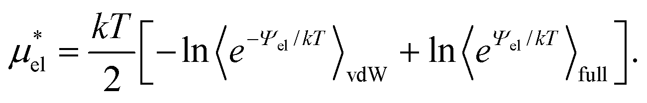 | (8) |
2.3
 ,
,  and
and 
The basic principle upon which one can understand qualitatively properties of a liquid near its triple point is that the short-range strong repulsive forces between molecules determine the structure of the liquid while the relatively long-range weak attractive forces exerted on a molecule by its neighbors largely cancel and thus basically provide the central molecule a deep uniform background potential.18 (This idea is the origin of what is called the van der Waals picture of liquids30 and naturally leads to the mean-field approximation of liquids, which we will also utilize below.) Therefore, it is a reasonable attempt to treat the attractive interactions between a solute molecule and solvent molecules by using the single-step perturbation method. The formation of a cavity in the solvent, on the other hand, should not be considered as a perturbation to the pure solvent. Following this physical reasoning, we always evaluate 


 using the thermodynamic integration method or the BAR method, both of which require simulations at many intermediate states, while we obtain
  and
and  by computing the right-hand sides of eqn (5) and (6), which require simulations at a single state.
The mean field approximation of liquids has been developed based on the basic principle described above. Using this approximation to the attractive part of the van der Waals interactions, eqn (5) is now
 | (9) |
 | (10) |
Similarly, if the structure of the solvent around the hypothetical nonpolar solute and that around the actual amphiphilic solute are basically the same, one would be able to approximate  by
by
 | (11) |
 | (12) |
In the present study, we will examine the validity of the mean-field approximations for temperature and pressure dependences of the solvation free energy of amphiphiles. It will be seen that eqn (10) is a good approximation while neither eqn (11) nor (12) is. The reason for the mean-field approximation for  being invalid is that the structure of the solvent around the hypothetical nonpolar solute and that around the amphiphilic solute are not basically the same. It is generally the case that
  .
.
A systematic way to improve the mean-field approximations for  is to make use of the following expression derived from the cumulant expansions31 of eqn (8),
 | (13) |
 | (14) |
3 Computational details
The solvation free energies of the two amphiphilic solutes and the potential energies for the solute–solvent interactions were obtained from isobaric–isothermal molecular dynamics (MD) simulations. The cubic simulation cell under the standard periodic boundary conditions contains one amphiphilic solute molecule, methanol or 1,2-hexanediol (HeD), and 1000 water molecules. The model water is the TIP4P/200534 and the model alcohols are of the TraPPE united atom force field.35–38 The alcohol–water site–site pair potentials are the sum of the Lennard–Jones (LJ) potential and the Coulombic potential. The LJ parameters for pairs of unlike interaction sites are those given by the Lorentz–Berthelot combining rule. The LJ potentials are truncated at 14 Å and the electrostatic interactions are calculated by the particle mesh Ewald method with a real space cut-off of 14 Å. The sides of the simulation box are always greater than twice the cut-off distance. The simulation time step is 1 fs. The temperature and pressure of the system are controlled by the Nosé–Hoover thermostat and the Parrinello–Rahman method. All the MD simulations were performed by GROMACS 2018.3.The solvation free energies and other quantities were obtained as a function of temperature at 1 bar and as a function of pressure at 300 K. The temperatures and pressures at which MD simulations were performed are as follows: T = 260, 280, 300, 320, 340, 360, 380, 400 K at 1 bar; p = 1, 1000, 2000, 3000, 6000 bar at 300 K.
The BAR method was employed for calculating μ* and  , separately. The results of the BAR method may be considered as the reference data with the highest accuracy. When calculating μ*, the BAR method was applied successively to
  and
and  , the sum of which gives μ*. The intermediate states for the calculation of
  are described by the pair potential between interaction sites of solute and water molecules:
 | (15) |
 , where the site–site pair potential is of the form:
 | (16) |
The  is the solvation free energy of a solute molecule which interacts with water molecules via the repulsive part of the Weeks–Chandler–Andersen (WCA) site–site pair potential,
 | (17) |
 we used 19 intermediate states in addition to the initial and final states. The intermediate site–site pair potential ϕWCA,λ(r) has a form analogous to eqn (15) and changes from 0 to ϕWCA(r) with λ varying from 0 to 1 with the interval of 0.05. At each intermediate state in the BAR calculations, a 1 ns equilibration run was followed by a 1 ns production run, and equilibrium configurations were sampled every 50 steps during the production run.
The average potential energies due to the solute–solvent attractive interactions were obtained from the MD simulations for the ensembles with the vdW and full potentials. In both ensembles, equilibrium configurations were sampled every 50 steps during a production run of 5 ns.
4 Results and discussion
4.1 Nonpolar contribution  as a function of T and p
Here we show the results for 
 , the nonpolar contribution to μ* as defined in eqn (3), and those for
  and
and  in eqn (4). The
  was obtained from the BAR method. We shall examine two routes to
  , i.e., one via the exact expression (5) and the other via the mean-field approximation (10) and discuss the temperature and pressure dependences of
  ,
,  , and
, and  .
.
Plotted in Fig. 1 are  ,
,  , and
, and  for the hypothetical nonpolar “methanol” in water, all divided by kT, as functions of temperature. It is seen that
  increases with temperature up to around 360 K and turns to decrease, which indicates that the solubility (the Ostwald absorption coefficient) is minimal at that temperature, a characteristic of hydrophobic hydration. The results of eqn (5) and (10) are in excellent agreement with those of the BAR method: the largest deviation from
  (BAR) is 0.17 at 260 K for eqn (5) and 0.45 at 260 K for eqn (10). The agreement of the mean-field result with the BAR result indicates that the basic principle in the theory of simple liquids holds even for the structure of water around nonpolar, polyatomic molecules and that the fluctuations in Ψattr are not significant.
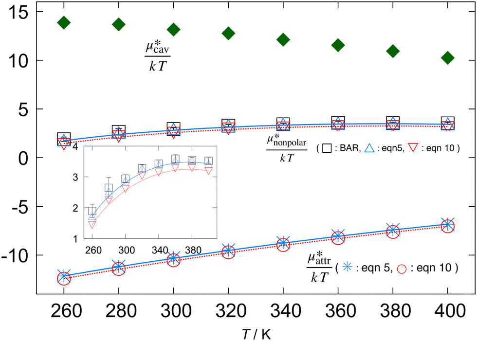 | ||
Fig. 1 Temperature dependences of  , ,  , and , and  for methanol in water at 1 bar. The inset shows the results for for methanol in water at 1 bar. The inset shows the results for  alone. alone. | ||
The plots in Fig. 1 also illustrate the following facts characteristic of the hydrophobic hydration: (i) A large positive value of  and a large negative value of
  largely cancel each other to give a small positive value of
  ; (ii)
  decreases monotonically with temperature and
  increases monotonically with temperature; and (iii) the concavity of
  with respect to temperature comes from the subtle difference between the temperature dependences of
  and
and  . The monotonic decrease of
  with increasing temperature at a fixed pressure is generally observed for any solute in water, and we will see the same trend for HeD in water as shown in Fig. 3(a). One can see this from the identity
  with Pcav being the probability of finding a cavity in water that can accommodate the solute molecule in question. This probability increases as the number density of water decreases. Therefore, as T increases at fixed p, the solvent density decreases, Pcav increases, and
  decreases.
Fig. 2 shows the pressure dependence of  for methanol along with those of
  and
and  . The pressure range is 1 to 6000 bar and the temperature is fixed at 300 K. The results obtained from the two routes to
  , eqn (5) and (10), are in good agreement with the BAR results: the largest deviation from
  (BAR) is 0.12 for eqn (5) and is 0.32 for eqn (10). As the pressure increases,
  increases monotonically while
  decreases monotonically; but the rate of change with pressure is much greater for
  than for
  , and so
  is only slightly smaller than the corresponding derivative of
  . Note that in general
  is the solvation volume v* = v − kTχ of the solute, where v is the partial molecular volume v and χ is the isothermal compressibility. Thus, we have
  and
and  for the nonpolar solute and the purely repulsive solute, respectively. Numerical values of
  and
and  for methanol in water are given in Table 1. Both the single-step perturbation method (5) and the mean-field approximation (10) give accurate values for
  in the wide range of pressure. It is generally true for any solute in water that
  is positive. One can see this also for HeD in water (Fig. 3(b)). As remarked in connection with the temperature dependence of
  ,
,  . Thus, as p increases, the solvent density increases, Pcav decreases, and
  increases.
 | ||
Fig. 2 Pressure dependences of  , ,  , and , and  for methanol in water at 300 K. for methanol in water at 300 K. | ||
| μ*/kT |
|
|
|
H*/kT | S*/k |
|
|
|
|---|---|---|---|---|---|---|---|---|
| Methanol | −8.37 | 13.2 | 2.94 | −11.3 | −16.8 | −8.43 | −11.3 | ∼0 |
| HeD | −14.4 | 33.3 | 5.21 | −19.6 | −37.3 | −22.8 | −23.5 | −3.83 |
| v*/10−2 nm3 |

|

|
||||||
| Methanol | 5.66 | 7.95 | 6.36 | |||||
| HeD | 18.3 | 25.7 | 20.1 | |||||


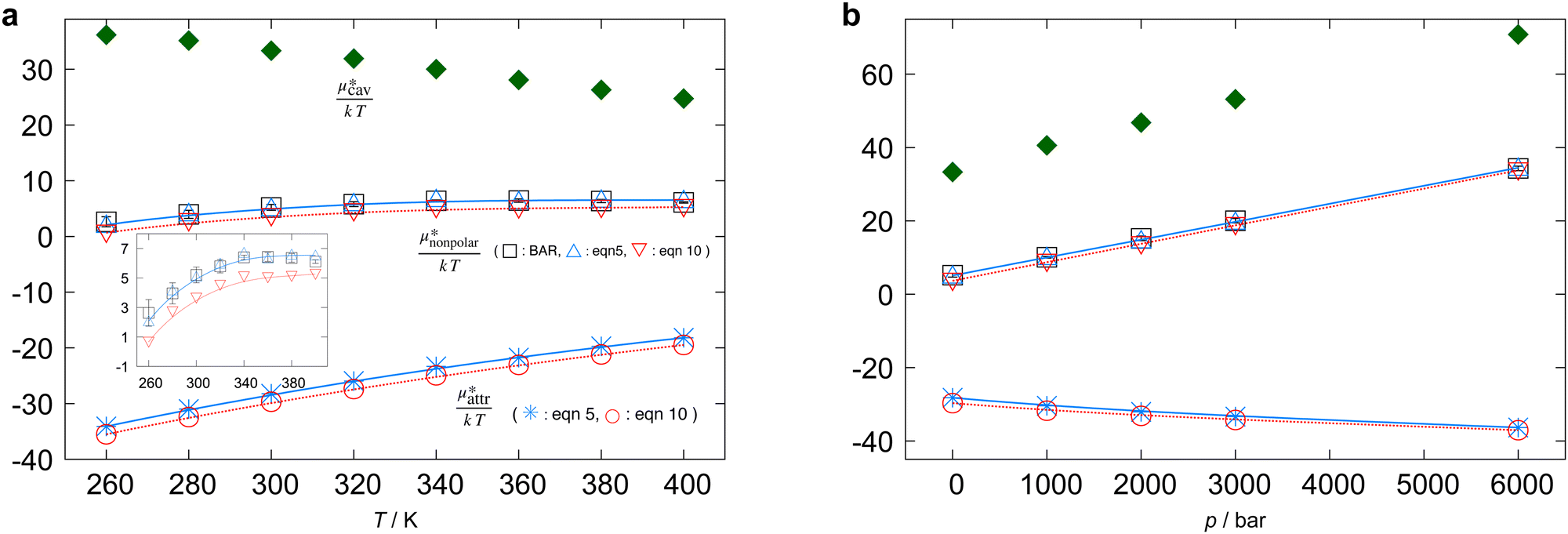 | ||
Fig. 3 Temperature and pressure dependences of  for HeD in water: (a) temperature dependence at 1 bar and (b) pressure dependence at 300 K. The results of BAR (□), the single-step perturbation (5) (Δ), and the mean-field approximation (10) (∇) are shown. The inset in (a) shows the results for for HeD in water: (a) temperature dependence at 1 bar and (b) pressure dependence at 300 K. The results of BAR (□), the single-step perturbation (5) (Δ), and the mean-field approximation (10) (∇) are shown. The inset in (a) shows the results for  alone. alone. | ||
The other amphiphilic solute, HeD, has a hydrophobic tail with six carbon atoms and two hydrophilic heads. Fig. 3a shows the temperature dependence of  ,
,  , and
, and  for HeD in water. The magnitude of
  at any given state is larger than that for methanol. This is simply because the molecular volume and surface area of HeD are larger. As a function of temperature,
  is concave downward and it is maximal at around 360 K, the same temperature as
  for methanol is maximal. The single-step perturbation method gives accurate results for
  ; the mean-field approximation underestimates
  . The largest deviation from the BAR results is 0.55 for eqn (5) and 1.97 for eqn (10). The apparent deviation of the mean-field approximation from the BAR result does not mean that the approximation for
  becomes invalid for large solutes; its relative accuracy remains the same for the two nonpolar solutes. The relative deviation
  is 2.5–4.9% for methanol and is 3.9–6.4% for HeD.
As seen in the insets in Fig. 1 and Fig. 3(a), the temperature dependence of  is greater for HeD than for methanol in the temperature range up to the temperature of maximum
  , which is close to 360 K. This is mainly due to the difference in molecular size. From the solvation thermodynamics, the following identity holds for any solute in any solvent: ∂(μ*/T)/∂T = −(1/T2)H*, where H* is the solvation enthalpy of the solute fixed in space under constant pressure and temperature. The larger the nonpolar solute the more negative the solvation enthalpy of the solute, because the dispersion interaction between a nonpolar solute and water molecules is stronger for a larger solute. For both methanol and HeD,
  is maximal at around 360 K. It might be a coincidence or it is possible that such a common temperature exists for a group of hydrocarbons.
Fig. 3b shows the pressure dependence of  for HeD. It increases linearly as the pressure increases. The result of eqn (5) is in good agreement with the BAR result, and the result of eqn (10) again underestimates the BAR result; but the deviation from the reference BAR data is at most 1.59 for the mean-field approximation (10). The value of
  for the “nonpolar” HeD is found to be three times larger than
  for methanol (Table 1).
Summarizing the above results, the use of eqn (5) for evaluating  proves to be very effective for both the small and large nonpolar solutes. The mean-field approximation, eqn (10), is less accurate than eqn (5). Furthermore, we confirmed that 〈Ψattr〉cav and 〈Ψattr〉vdW are, respectively, smaller (more negative) and greater (less negative) than the exact value of
  , which is consistent with the Gibbs-Bogoliubov inequality,39,40
| 〈Ψattr〉cav ≤ kTln〈eΨattr/kT〉vdW ≤ 〈Ψattr〉vdW. | (18) |
4.2 Electrostatic contribution  as a function of T and p
The electrostatic contribution 
 is the difference in the solvation free energy between the solute of interest and the hypothetical nonpolar one. One could in principle evaluate
  using either eqn (6), (7), (11), or (12). These routes to
  are much more efficient than the BAR method. In practice, however, their results would notably deviate from the accurate BAR results. Here we examine three methods for calculating
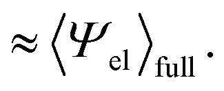
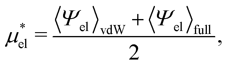
  . The first method is to use eqn (8). We call it the perturbation combining method (PC) as eqn (8) combines the two exact perturbation formulae. The PC method is expected to be more accurate than the forward or reverse perturbation method because numerical errors for the two perturbation methods cancel each other out to some extent when combined. The second method is the linear response (LR) approximation (14). The LR method is effective for ionic solutes but not for polar ones.32 An empirical way to improve eqn (14) is to replace 1/2 in the equation by some parameter β, i.e., to employ
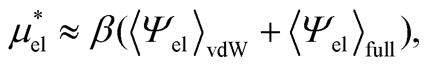 | (19) |
Fig. 4 shows temperature and pressure dependences of  for methanol in water as obtained from the PC, LR, mLR, and BAR methods. It is found that the PC method gives overall accurate results: the largest deviation from the BAR data is 1.65 for the temperature dependence and 1.34 for the pressure dependence. On the other hand, the LR method gives consistently lower values than the BAR results both for temperature and pressure dependences. This indicates that the variance of the Coulomb potential energy in the ensemble with the vdW potential is largely different from that in the ensemble with the full potential. The results of the mLR method (βmethanol = 0.374) are in good agreement with the BAR results: the largest deviation, in units of kT, is 0.966 and 0.442 for the temperature and pressure dependence, respectively.
 | ||
Fig. 4 Temperature and pressure dependence of  , the electrostatic contribution to the solvation free energy of methanol in water: (a) , the electrostatic contribution to the solvation free energy of methanol in water: (a)  vs. T at 1 bar and (b) vs. T at 1 bar and (b)  vs. p at 300 K. The results of the perturbation combining (eqn (8)), linear response (eqn (14)), modified linear response (eqn (19)) methods, and the numerically exact results (black squares) are plotted. The parameter βmethanol in eqn (19) is 0.374, which was determined at 300 K and 1 bar. vs. p at 300 K. The results of the perturbation combining (eqn (8)), linear response (eqn (14)), modified linear response (eqn (19)) methods, and the numerically exact results (black squares) are plotted. The parameter βmethanol in eqn (19) is 0.374, which was determined at 300 K and 1 bar. | ||
Fig. 5 shows the temperature and pressure dependence of  of HeD in water. As in the case of methanol, the LR method is the least accurate among the three. The mLR method (βHeD = 0.347) reproduces the BAR results very well for both the temperature and pressure dependence. The largest deviation from the BAR results is 1.20 and 0.387 for the temperature and pressure dependence, respectively. The PC method, which has no adjustable parameter, gives overall much more accurate results than the LR method. The largest deviation from the BAR values is 2.90 and 2.66 for the temperature and pressure dependence, respectively.
 | ||
Fig. 5 Temperature and pressure dependence of  of HeD in water: (a) of HeD in water: (a)  vs. T at 1 bar and (b) vs. T at 1 bar and (b)  vs. p at 300 K. The results of the perturbation combining (eqn (8)), linear response (eqn (14)), modified linear response (eqn (19)) methods, and the numerically exact results (black squares) are plotted. The parameter βHeD in eqn (19) is 0.347, which was determined at 300 K and 1 bar. vs. p at 300 K. The results of the perturbation combining (eqn (8)), linear response (eqn (14)), modified linear response (eqn (19)) methods, and the numerically exact results (black squares) are plotted. The parameter βHeD in eqn (19) is 0.347, which was determined at 300 K and 1 bar. | ||
The temperature derivatives  for methanol and HeD at 300 K are found to be 0.0377 K−1 and 0.0783 K−1, respectively. The ratio of these values is close to 1:2, which coincides with the ratio of the number of OH groups in these alcohols. This suggests that the contribution of each hydrophilic group to
  is additive.
4.3 The solvation free energy μ* as a function of T and p
We present here the solvation free energy for methanol and HeD in water as a function of T and p. Remember that
  is further divided into
  and
and  . The results for μ* are those obtained from three methods. Since
  was evaluated using the BAR method in any case, the three methods differ only in the ways of evaluating
  and
and  . In the first method,
  is calculated by eqn (5) and
  by eqn (8), thus the method uses exact relationships only. We shall refer to the first route to μ* as the PC method. In the second method, which is referred to as the mean-field + linear response (MF + LR) method,
  is evaluated by eqn (10) and
  is calculated by eqn (14). Finally in the third method, which we call the mean-field+ modified linear response (MF + mLR) method,
  is evaluated by eqn (10) and
  by eqn (19).
Fig. 6 shows μ*/kT for methanol in water as a function of temperature and pressure. The results of the MF + mLR method are in excellent agreement with those of the BAR method for the wide ranges of temperature and pressure. It is because the mean-field approximation is very effective for nonpolar solutes and because the modified linear response method has a single adjustable parameter β. The results derived from the PC method are in good agreement with the BAR results. The MF + LR method gives overall the least accurate results. The reason is, as we saw above, that the linear response method for the electrostatic contribution gives large errors. In the PC method, the largest deviation from the BAR result is 1.66 for the temperature dependence and 1.40 for the pressure dependence; in the MF + mLR method, it is 0.97 for the temperature dependence and 0.44 for the pressure dependence. We note that the maximum of  with respect to T in the temperature range disappears when the electrostatic contribution is added.
 | ||
| Fig. 6 Temperature and pressure dependence of μ*, the total solvation free energy for methanol in water: (a) μ*/kT vs. T at 1 bar and (b) μ*/kT vs. p at 300 K. The result of the perturbation combining (PC), the mean-field approximation + linear response (MF + LR), the mean-field approximation + modified linear response (MF + mLR) methods, and the numerically exact results (black squares) are plotted. The parameter βmethanol in the modified linear response method is 0.374, which was determined such that eqn (19) holds exactly at 300 K and 1 bar. | ||
Fig. 7 shows the results for HeD. The relative degrees of accuracy of the three methods are the same as those for methanol. With the PC method the largest deviation from the exact results is 2.89 and 2.65 for the temperature and pressure dependence, respectively; In the MF + mLR it is 1.20 and 0.39 for the temperature and pressure dependence, respectively. It is found that μ*/kT as a function of T does not exhibit a maximum in the temperature range. We have observed in Fig. 3 that there is a maximum of  in the same temperature range. The absence of the maximum of μ*/kT is due to the near-linear temperature dependence of
  (Fig. 5). It has been remarked by Cerdeiriña and Debenedetti41 that the temperature of the maximum density of water is a necessary condition for the solubility minimum or, equivalently, the maximum of μ*/kT; but it is not a sufficient condition as one finds no solubility minima for alcohols in water.
 | ||
| Fig. 7 Temperature and pressure dependence of μ* of HeD in water: (a) μ*/kT vs. T at 1bar and (b) μ*/kT vs. p at 300 K The result of the perturbation combining (PC), the mean-field approximation + linear response (MF + LR), the mean-field approximation + modified linear response (MF + mLR) methods, and the numerically exact results (black squares) are plotted. The parameter βHeD in the modified linear response method is 0.374, which was determined such that eqn (19) holds exactly at 300 K and 1 bar. | ||
For HeD, the results from the PC and MF + mLR methods are very close to each other (Fig. 7(a)), but this might be a mere coincidence. On the other hand, for methanol, the difference between two sets of results from the two methods becomes larger at lower temperatures (Fig. 6), and the same trend is found for  in Fig. 4.
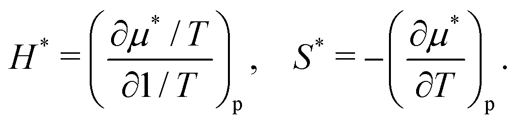
Table 1 lists the solvation thermodynamic quantities for the two alcohols. The temperature derivatives of μ* are related to changes in the enthalpy and entropy associated with the solvation process in which the volume of the system changes by v*:
 | (20) |
 and entropy
  defined in ref. 42. The latter two are defined for the solvation process in which the volume changes by the partial molecular volume vp. The numerical results in Table 1 demonstrate that μ* for each alcohol is negative because H* is more negative than TS* in contrast to the fact that μ* for a nonpolar solute is positive because H* is less negative than TS*. We also evaluated
  and
and  , which are analogously defined by the temperature derivatives of
  . Note that
  for HeD is approximately twice as large as that for methanol. This is mainly due to the fact that HeD has two OH groups while methanol has one, and this explains our earlier observation that the slope of
  against T is twice larger for HeD than for methanol. As regards the solvation volume, we find that
  and
and  for both alcohols. The contributions of the vdW forces and the electrostatic interactions are respectively
  and
and  . For each alcohol,
  , i.e., the effect of the van der Waals interactions on the reduction of
  is greater than the effect of the electrostatic interactions on the reduction of
  .
.
5 Conclusions
The solvation free energies μ* of amphiphilic solute species, methanol and HeD, in water were calculated as functions of temperature and as those of pressure. The solvation process of any amphiphile may be divided into three steps, cavity formation in water (insertion of a purely repulsive molecule in the solvent), addition of the van der Waals attractive force to the repulsive solute–water interactions, and addition of the electrostatic interactions to the nonpolar solute–water interactions. The first, second, and third steps give ,
,  , and
, and  , respectively. The sum of the first two is the solvation free energy
  of the hypothetical nonpolar solute and the sum of the three is μ*.
We assessed the relative accuracy of the free-energy calculation methods based on exact and approximate formulae with respect to the accurate yet time-consuming BAR method. The following conclusions were derived.
First, the mean-field approximation, eqn (10), works reasonably well for polyatomic nonpolar solutes as large as the size of hexanediol. Its validity is known for the hydration of small solutes such as methane but it has not been checked for larger nonpolar solutes before. The relative errors in  to the exact results are more or less the same for the two solutes: 2.5–4.9% for methanol and 3.9–6.4% for HeD. This indicates that the basic assumption holds for complex, nonpolar solutes in water, i.e., the structure of solvent molecules around a solute is basically determined by the strong, short-range repulsive forces between solute and solvent molecules.
Second, unlike  , one cannot evaluate accurately the contribution
  of the electrostatic interactions using the mean-field approximation and the single-step perturbation. The modified linear response (mLR) method, eqn (19), best reproduces the temperature and pressure dependences of
  , but it should be noted that it has one fitting parameter β. On the other hand, the perturbation combining method, eqn (8), with no fitting parameter works sufficiently well over the wide ranges of temperature and pressure.
Third, we assessed the three methods, MF + LR, MF + mLR, and PC, to calculate  . In the first two methods “MF” denotes the mean-field approximation for
  and the “LR” and “mLR” represent the linear response and modified linear response approximations for
  . The PC method uses the perturbation method for
  and the perturbation combining formulae for
  . Overall, both the MF + mLR and PC methods are able to reproduce equally well the temperature and pressure dependences of μ*, but given the fact that the former relies on the approximation for
  with the fitting parameter, one may conclude that the PC method is superior to the other approximations. We note that the success of the PC method is due to the cancellation of errors in the two terms in eqn (8). If the PC method is found to be effective for solute species with different sizes, shapes, and degrees of hydrophobicity, we could employ it instead of the commonly used BAR method. Its applicability to a variety of amphiphiles must be examined in future work.
The division of μ* into  ,
,  , and
, and  helps us understand the temperature and pressure dependences of μ* of alcohols in water. In general, there is the temperature of maximum μ*/kT for a nonpolar solute in water, or equivalently the temperature of the solubility minimum (the Ostwald absorption coefficient) at atmospheric pressure; however, μ*/kT for an amphiphile with one or two OH groups monotonically increases. This is because
  is near-linear in T,
  is a concave function of T with a maximum at some temperature, and the electrostatic term is sufficiently large to suppress the otherwise existing maximum.
The solvation volume v*, the pressure derivative of μ* at fixed T, is nearly constant for both alcohols in the wide range of pressures. The main factor determining v* is  as anticipated and the electrostatic interaction has the smallest contribution to v*. The ratios of
  ,
,  , and v* for methanol and HeD is found to be the same:
 . We believe that the coincidence is due to a particular choice of the two alcohols. We also find that the value of
  of HeD is approximately twice larger than that of methanol. This seems to suggest that the contributions of hydrophilic groups to the solvation enthalpy are additive. This hypothesis should be checked by experiment for dilute aqueous solutions of amphiphiles.
Author contributions
A. Taira and K. Koga conceived the work and developed the proposed methods. A. Taira implemented the method and performed the MD simulations and numerical analyses. They wrote the draft of the manuscript. All the authors, A. Taira, R. Okamoto, T. Sumi, and K. Koga, contributed to the discussion and finalizing the manuscript.Conflicts of interest
There are no conflicts to declare.Acknowledgements
The computation was performed at the Research Center for Computational Science, Okazaki, Japan (Project: 21-IMS-C125, 22-IMS-C124, 23-IMS-C112). This work was supported by JSPS KAKENHI (grant no. 18KK0151 and 20H02696) and JST, the establishment of university fellowships towards the creation of science technology innovation (grant no. JPMJFS2128).References
- S. H. Fleischman and C. L. Brooks III, J. Chem. Phys., 1987, 87, 3029–3037 CrossRef CAS.
- E. M. Duffy and W. L. Jorgensen, J. Am. Chem. Soc., 2000, 122, 2878–2888 CrossRef CAS.
- S. Wan, R. H. Stote and M. Karplus, J. Chem. Phys., 2004, 121, 9539–9548 CrossRef CAS PubMed.
- M. M. Kubo, E. Gallicchio and R. M. Levy, J. Phys. Chem. B, 1997, 101, 10527–10534 CrossRef CAS.
- A. Ben-Naim, Solvation Thermodynamics, Plenum, New York, 1987 Search PubMed.
- B. Guillot and Y. Guissani, J. Chem. Phys., 1993, 99, 8075–8094 CrossRef CAS.
- B. Lee, Biophys. Chem., 1994, 51, 271–278 CrossRef CAS PubMed.
- V. A. Payne, N. Matubayasi, L. R. Murphy and R. M. Levy, J. Phys. Chem. B, 1997, 101, 2054–2060 CrossRef CAS.
- S. Garde, A. E. García, L. R. Pratt and G. Hummer, Biophys. Chem., 1999, 78, 21–32 CrossRef CAS PubMed.
- S. W. Rick, J. Chem. Phys., 2000, 104, 6884–6888 CrossRef CAS.
- T. Ghosh, A. E. García and S. Garde, J. Am. Chem. Soc., 2001, 123, 10997–11003 CrossRef CAS PubMed.
- K. Koga, J. Chem. Phys., 2004, 121, 7304–7312 CrossRef CAS PubMed.
- K. Abe, T. Sumi and K. Koga, J. Phys. Chem. B, 2016, 120, 2012–2019 CrossRef CAS PubMed.
- K. Koga and N. Yamamoto, J. Phys. Chem. B, 2018, 122, 3655–3665 CrossRef CAS PubMed.
- C. A. Cerdeiriña and B. Widom, J. Phys. Chem. B, 2016, 120, 13144–13151 CrossRef PubMed.
- C. H. Bennett, J. Comput. Phys., 1976, 22, 245–268 CrossRef.
- J. P. Hansen and I. R. McDonald, Theory of simple liquids: with applications to soft matter, Academic Press, 4th edn, 2013 Search PubMed.
- B. Widom, Science, 1967, 157, 375–382 CrossRef CAS PubMed.
- J. Åqvist, C. Medina and J.-E. Samuelsson, Prot. Eng., 1994, 7, 385–391 CrossRef PubMed.
- H. S. Ashbaugh and B. A. Pethica, Langmuir, 2003, 19, 7638–7645 CrossRef CAS.
- B. Widom, J. Chem. Phys., 1963, 39, 2808–2812 CrossRef CAS.
- R. W. Zwanzig, J. Chem. Phys., 1954, 22, 1420–1426 CrossRef CAS.
- H. Liu, A. E. Mark and W. F. van Gunsteren, J. Phys. Chem., 1996, 100, 9485–9494 CrossRef CAS.
- J. W. Pitera and W. F. V. Gunsteren, J. Phys. Chem. B, 2001, 105, 11264–11274 CrossRef CAS.
- W. F. Van Gunsteren, X. Daura and A. E. Mark, Helv. Chim. Acta, 2002, 85, 3113–3129 CrossRef CAS.
- C. Oostenbrink, in Computational drug discovery and design, Springer, 2012, pp. 487–499 Search PubMed.
- C. Oostenbrink and W. F. van Gunsteren, Proteins: Struct., Funct., Genet., 2004, 54, 237–246 CrossRef CAS PubMed.
- C. Oostenbrink and W. F. van Gunsteren, Proc. Natl. Acad. Sci. U. S. A., 2005, 102, 6750–6754 CrossRef CAS PubMed.
- J. Aqvist, V. B. Luzhkov and B. O. Brandsdal, Acc. Chem. Res., 2002, 35, 358–365 CrossRef PubMed.
- D. Chandler, J. D. Weeks and H. C. Andersen, Science, 1983, 220, 787–794 CrossRef CAS PubMed.
- R. Kubo, J. Phys. Soc. Jpn., 1962, 17, 1100–1120 CrossRef.
- J. Åqvist and T. Hansson, J. Phys. Chem., 1996, 100, 9512–9521 CrossRef.
- M. Almlöf, J. Carlsson and J. Åqvist, J. Chem. Theory Comput., 2007, 3, 2162–2175 CrossRef PubMed.
- J. L. Abascal and C. Vega, J. Chem. Phys., 2005, 123, 234505 CrossRef CAS PubMed.
- B. Chen, J. J. Potoff and J. I. Siepmann, J. Phys. Chem. B, 2001, 105, 3093–3104 CrossRef CAS.
- M. G. Martin and J. I. Siepmann, J. Phys. Chem. B, 1998, 102, 2569–2577 CrossRef CAS.
- M. G. Martin and J. I. Siepmann, J. Phys. Chem. B, 1999, 103, 4508–4517 CrossRef CAS.
- J. M. Stubbs, J. J. Potoff and J. I. Siepmann, J. Phys. Chem. B, 2004, 108, 17596–17605 CrossRef CAS.
- R. Underwood and D. Ben-Amotz, J. Chem. Phys., 2011, 135, 201102 CrossRef PubMed.
- A. Isihara, J. Phys. A: Gen. Phys., 1968, 1, 539 CrossRef.
- C. A. Cerdeiriña and P. G. Debenedetti, J. Chem. Phys., 2016, 144, 164501 CrossRef PubMed.
- K. Koga, Phys. Chem. Chem. Phys., 2011, 13, 19749 RSC.
| This journal is © the Owner Societies 2023 |